Improving 3-m Resolution Land Cover Mapping through Efficient Learning from an Imperfect 10-m Resolution Map

Abstract

Substantial progress has been made in the field of large-area land cover mapping as the spatial resolution of remotely sensed data increases. However, a significant amount of human power is still required to label images for training and testing purposes, especially in high-resolution (e.g., 3-m) land cover mapping. In this research, we propose a solution that can produce 3-m resolution land cover maps on a national scale without human efforts being involved. First, using the public 10-m resolution land cover maps as an imperfect training dataset, we propose a deep learning based approach that can effectively transfer the existing knowledge. Then, we improve the efficiency of our method through a network pruning process for national-scale land cover mapping. Our proposed method can take the state-of-the-art 10-m resolution land cover maps (with an accuracy of 81.24% for China) as the training data, enable a transferred learning process that can produce 3-m resolution land cover maps, and further improve the overall accuracy (OA) to 86.34% for China. We present detailed results obtained over three mega cities in China, to demonstrate the effectiveness of our proposed approach for 3-m resolution large-area land cover mapping.

1. Introduction

Land cover mapping, as a basic process to categorize and describe the surface on Earth, provides fundamental data for various management and research applications, such as food production forecast, urban planning, flood control, disaster prevention, biodiversity protection, climate change research, and other Earth system studies [1]. With the demand of detailed land resource surveys and spatial planning for optimizing the development and protection of national land space, high-resolution land cover data is significant and widely used in many sustainability-related applications [2]. Its uses include modeling un-authorized land use sprawl, monitoring urban changes and surveying the coastline [3]. The potential of 1–3 m resolution land cover data opens the door to many new applications that require high geometric precision and roof-top/small-farm level spatial details. Therefore, timely and higher resolution land cover products are urgently needed [4].

In the past few decades, thanks to the advancement in satellite remote sensing and data processing technologies, more and more higher resolution land cover products have been produced at the global and continental scales [2,4]. At the global scale, 1-km spatial resolution land cover products have been developed using Advanced Very High Resolution Radiometer (AVHRR) data [5,6]. Annual 500-m resolution global land cover products were developed for several generations [7,8]. In 2008, ESA delivered the first 300-m resolution global land cover maps for 2005 [9]. Then in 2011, ESA and the Université catholique de Louvain (UCL) delivered a set of GlobCover 2009 products [10]. The CCI-LC team produced and released its 3-epoch series of global land cover maps at a 300-m spatial resolution, where each epoch covers a 5-year period (2008–2012, 2003–2007, 1998–2002) [11]. In 2013, the first 30-m resolution global land cover maps were produced using Landsat Thematic Mapper (TM) and Enhanced Thematic Mapper Plus (ETM+) data [1]. In 2019, the latest global land cover product, Finer Resolution Observation and Monitoring of Global Land Cover (FROM-GLC10), developed with 10-m resolution Sentinel-2 data for 2017, was published [4]. Over the recent decades, these public land cover datasets have already made significant contributions to the global research community. Taking the FROM-GLC series of datasets as an example, the 30-m and 10-m results have already been accessed by over 50,000 users from 183 different countries, with over 30 million file clicks and downloads (http://data.ess.tsinghua.edu.cn/).

In recent years, with the increased availability of high-resolution remotely sensed data, the maturing of machine learning techniques (especially deep learning based methods), and the readiness of computing capabilities, land cover mapping efforts have been further extended to a resolution of three meters or even one meter [12,13]. However, under the current paradigm of deep neural networks, one major constraint that stops many researchers from achieving improved results is the lack of well-labelled training data [14].

If we look at the recent boom in deep learning technologies in the domain of computer vision, a critical base is the availability of many well-labeled datasets like ImageNet [15]. However, remote sensing images are more diverse and more difficult to interpret than daily images. Because the interpretation and labelling of remotely sensed images requires huge human efforts and a high level of expertise, it is costly and time-consuming to obtain high-resolution land cover maps on a large scale. Although many efforts have been devoted to developing land cover datasets on a large scale [1,16], they suffer from a number of limitations, such as point-based or patch-based annotation, diversity or simplification of the samples and the scenes, variation in the spatial resolution, and hardly accessible or unpublished datasets. For example, it took 10 months and $1.3 million to label about 160,000 square kilometers in the Chesapeake Bay watershed in the northeastern United States that included only four cover types (Water, Forest, Field, and Impervious) [17]. Even with those high-cost and numerous interpretation datasets, the limited number of land cover types and the specific coverage make it difficult to use for other land cover studies [2]. Gong et al. [4] transformed a 30-m resolution sample set, which is a point-based annotation at the global scale, to mapping, at a 10-m resolution, global land cover with more spatial detail yet found no accuracy improvement. The reason is that the spatial resolution and point-based annotation of the 30-m land cover dataset presents a strong limitation to higher resolution land cover mapping.

To deal with the above-mentioned issues, many recent studies have focused on training data collection from readily available land cover products. For instances, Zhang et al. used the random forest classification method to transfer a 500-m resolution MODIS (the Moderate Resolution Imaging Spectroradiometer) land cover product to produce 30-m land cover classification results in North America [18]. Lee et al. applied an improved Bayesian Updating of Land Cover algorithm to sharpen the results from a 300-m to a 30-m classification [19]. Zhang et al. combined the MODIS and GlobCover2009 land cover product to produce a 30-m resolution land cover map of China [20]. Although they have demonstrated that refined 30-m resolution land cover maps can be produced from lower resolution land cover products, the feasibility of transferring the knowledge to a very high resolution (e.g., 3-m) has never been assessed. Schmitt et al. integrated 10-m resolution images (Sentinel-1 and Sentinel-2) with low-resolution MODIS land cover (with 250-m to 1000-m resolution) to produce the higher resolution SEN12MS dataset [21]. This problem was defined as weakly supervised learning for land cover prediction due to the huge difference in resolution between the MODIS land cover products and satellite data [22]. However, in this work, we explore the possibility of transferring a 10-m product to produce 3-m results, in which satellite images and land cover products are both in higher resolutions and have relatively small resolution gaps. The situation and corresponding methodology are quite different from the above studies, because of the characteristics of different resolution satellite imagery and the accuracy of different land cover products.

Open Street Map (OSM) or other open data sources were also used in updating and improving land cover and land use products [23,24]. Kaiser et al. indicated that the use of large-scale imperfect labeled training data could replace 85% of high-quality manually labeled data in high-resolution building and road extraction [23]. An impressive performance in the imperfect label situation has been achieved, which only drops by 6% in accuracy when the proportion of imperfect labels increases up to 50% [25]. These studies show that in specific scenarios or cases, even though training on imperfect data, it may still achieve reasonable results [26]. Based on the existing efforts mentioned above, we propose a deep learning based approach that can intelligently and efficiently “grow” the current 10-m resolution FROM-GLC land cover product to an improved 3-m resolution land cover product.

The first part of this research focuses on designing a robust and generalized learning method that can take advantage of the imperfect 10-m resolution product as the training input, and transfer the knowledge into a network that can produce refined 3-m resolution land cover maps. In recent years, deep learning-based approaches for high-resolution land cover mapping have been considered as the state-of-the-art methods [2,12]. High-resolution satellite imagery contains more spatial information (e.g., texture, contexture, and shape). A deep learning-based semantic segmentation method can effectively extract the necessary spatial information from the neighborhoods surrounding each pixel. It enables effective end-to-end segmentation, obtaining superior results to traditional machine learning methods and the patch-based Convolutional Neural Network (CNN) classification method [27]. For example, on the ISPRS Vaihingen benchmark (including six types, i.e., impervious surface, building, low vegetation, tree, car, and background), Audebert et al. [28] achieved an overall accuracy of 89.8%, which is over 3.9% higher than that with traditional machine learning methods, such as Random Forest (RF) with a fully connected conditional random field (CRF). Liu et al. [29] proposed a self-cascaded network based on PSPNet [30] and RefineNet [31], which further improved the overall accuracy to 91.1% for the ISPRS Vaihingen challenge online test dataset in 2017. The latest national-scale 1-m resolution land cover maps (using aerial imagery from the USDA National Agriculture Imagery Program) of the US in 2019 applied the U-Net Large model and achieved substantially improved results (with an overall accuracy increased by 2%–41% in different test regions) compared with a traditional machine learning method (i.e., RF) [2]. As a result, we apply a deep learning-based semantic segmentation method for this research.

The second part of this research focuses on improving the computational efficiency of the proposed method. Recent studies on model compression and acceleration include Quantization [32], Fast convolution [33], Low rank approximation [34], and Filter pruning [35]. In this study, we apply filter pruning due to its usability and expansibility. Aiming at producing a continental or even global land cover product, we carefully prune the resulting segmentation model so that we can process an area as big as China within a few days rather than a few months. The basic idea of our pruning method is to remove the redundant or insignificant filters in the network that make little or no contribution to the final output [29,36]. For example, He et al. proposed the Soft Filter Pruning (SFP) method, which reduced FLOPs by more than 40.8% on ResNet-110 and even produced a 0.18% accuracy improvement on CIFAR-10 [37]. Filter Pruning via Geometric Median (FPGM) [3] was proposed in 2019, and further reduced FLOPS by more than 52% on ResNet-110 and even produced a 2.69% relative accuracy improvement on the same dataset. In our work, we explored the pruning of a rather complex architecture (i.e., high-resolution network [38]) compared with ResNet, implemented on a more complicated dataset compared to CIFAR-10. We apply FPGM for network compression and acceleration with almost no loss of accuracy. This makes it possible to map large areas.

In summary, we aim to produce a novel 3-m resolution land cover map through efficient learning from imperfect 10-m resolution maps without any human interpretation. We propose a complete workflow and a deep learning-based network for this task, which is beneficial to reduce the research thresholds in this community and serves as an example to similar studies. Furthermore, we exhibit the 3-m resolution land cover mapping results over three cities in China as examples (i.e., Harbin, Taiyuan, and Shanghai) to demonstrate the effectiveness of our proposed approach for 3-m resolution large-area land cover mapping.

2. Data

2.1. Image Data Source

All satellite images used in this study were acquired from Planet satellites at 3-m resolution with four bands (R, G, B, NIR). Planet’s constellation of satellites orbits the poles every 90 min, capturing the entire Earth’s landmass every day. Radiometric correction was applied to the data. Images were orthorectified and projected to a Universal Transverse Mercator (UTM) projection. Planet satellite images were downloaded through Planet API (https://www.planet.com/products/platform), which has a screening function for clouds. Users can easily exclude images whose cloud coverage exceeds a specified percentage. Planet images of the sample datasets were acquired in June, 2017 with less than 15% cloud cover, matching the time of the 10-m resolution land cover product. Each image tile has a size of 8000 × 8000 pixels. While the model was trained using 2017 images, we chose to use images in 2018 to produce urban maps in China, so as to provide a more up-to-date land cover product.

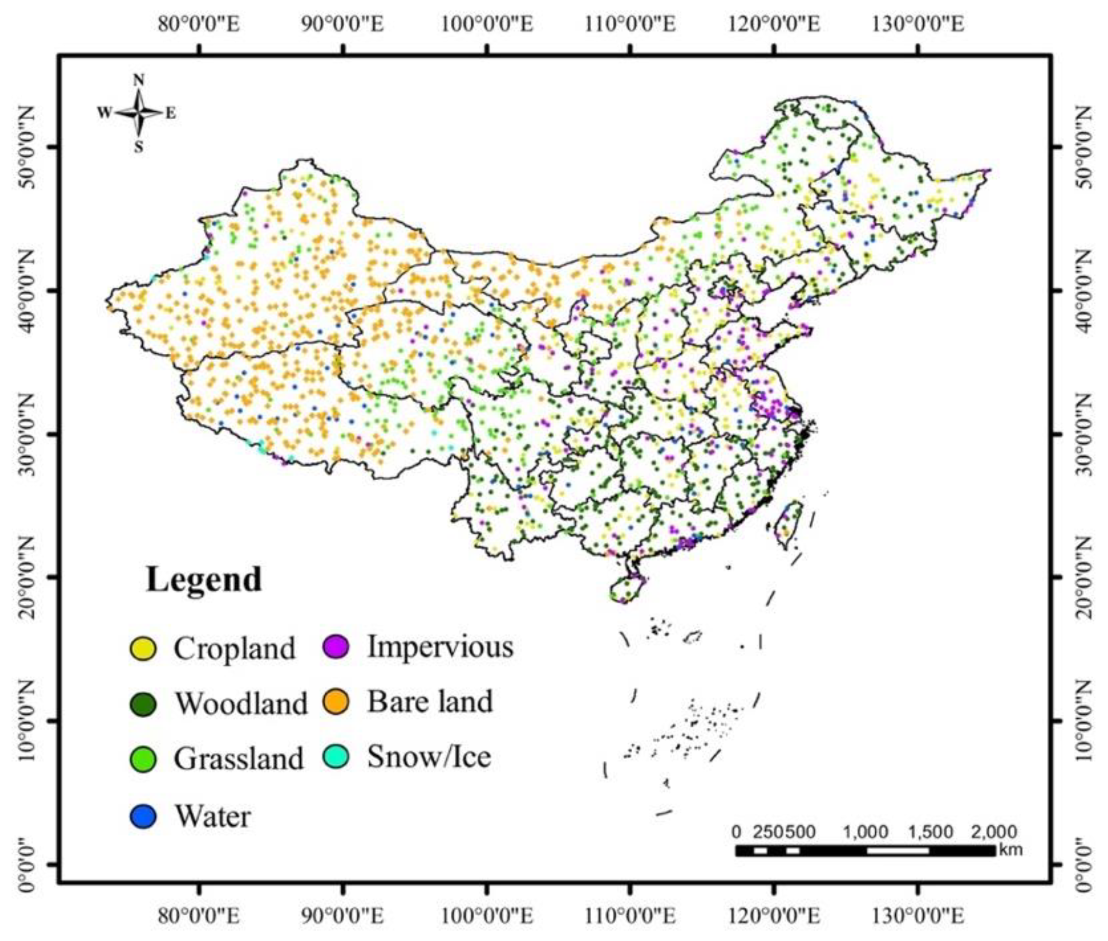
2.2. Label Data Source and Classification System

The supervised labeling of the training and validation datasets in this paper was the latest public global land cover product, Finer Resolution Observation and Monitoring of Global Land Cover (FROM-GLC10), which maps 10-m resolution global land cover in 2017 [4]. FROM-GLC10 was downloaded through the website (http://data.ess.tsinghua.edu.cn), and each downloaded tile has 22,265 × 22,265 pixels. It includes ten land cover types (i.e., Cropland, Forest, Grassland, Shrubland, Wetland, Water, Tundra, Impervious, Bare land, and Snow/Ice) and achieves an overall accuracy of 72.8% at the global scale. FROM-GLC10 was produced by a random forest classifier using the multispectral Sentinel-2 image with four 10-m resolution visible and near infrared bands, and six 20-m resolution red-edge and middle infrared spectral bands. The mapping results of FROM-GLC10 in China were used in this study as the imperfect labels.

Based on the global land-cover classification system of FROM-GLC [1] and the national land-cover classification system in China [39], we classified the land cover into seven types in China (i.e., Cropland, Woodland, Grassland, Water, Impervious, Bare land, and Snow/Ice). As tundra in the global land-cover classification system are very few in China, they were not included into our classification systems. The definition of the difference between Forest and Shrubland is whether the height exceeds five meters in the global land-cover classification system [1]. They are easily confused without rich morphological information. Thus, we merged Forest and Shrubland into a single class of Woodland. In addition, wetland is highly variable over time, so using a single date image as in our work would not result in accurate classification. Due to the relatively low coverage (less than 3% of China’s territory) and high spectral variability of wetlands in China, this type was also not included in our classification systems. Wetland and Tundra in FROM-GLC10 were set as background and ignored during the training phase.

2.3. Datasets

The training and validation datasets used in this study were built based on the Planet images and FROM-GLC10, covering one-third of the territory of China, which was randomly selected from the whole of China. First, the Planet images were cropped into chips of 1024 × 1024 pixels and matched with the corresponding FROM-GLC10 result tiles through their geographic coordinates. Thereafter, the coordinate system of FROM-GLC10 (i.e., the WGS-84 coordinate system) was re-projected onto the coordinate system of the Planet image (i.e., Universal Transverse Mercator Projection), so that the FROM-GLC10 tile could be cropped and re-sampled (by nearest neighbor interpolation) to a size of 1024 × 1024 pixels, exactly matching the corresponding Planet image chip. Thus, we could obtain the paired satellite image and land cover label as the original dataset, as shown in Figure 1. Then, we randomly selected 100,000 training data and 2000 validation data from the original dataset as the preliminary dataset. For better usage of FROM-GLC10, it is reasonable to use the portion of FROM-GLC10 with relatively high accuracy and remove the poor quality portion. Therefore, we filtered out the poor quality portion of the original dataset according to the preliminary land cover mapping results. Specifically, we used the original dataset to train a preliminary model, and the model is described in Section 3.2. Then, we used the trained model to predict the land cover mapping results for each training image. The similarity between our mapping result and the FROM-GLC10 result of each image was calculated, which is defined as the number of same classified pixels divided by the total number of pixels in the image. On the imperfect dataset, lower similarities are more likely to represent poor quality results instead of samples that are difficult to learn. Therefore, we filtered out the original dataset whose similarity was below 20%. The remaining data were divided into training and validation sets. The final size of training and validation datasets are 50,000 and 2000, respectively. In addition, in order to increase data diversity and match the input size of the network, the input images were cropped to 513 × 513 pixels in every training epoch.

The test dataset was built based on the published global land cover validation sample in 2015 [40], which contains 35,011 sample units for ten types at the global scale. We only used 1692 sample units for seven types (i.e., Cropland, Woodland, Grassland, Water, Impervious, Bare land, and Snow/Ice) in China, where the sample units of Woodland were obtained by combining the sample units of Forest and Shrubland. As the number of the sample units for Water and Impervious is rather small, we supplemented 248 additional sample units of these two types by randomly generating coordinate points on the published water, building, and road extraction results from Open Street Map. In addition, as the published sample units were collected from the 30-m resolution satellite images in 2015, we reinterpreted the test dataset for 3-m resolution satellite images in 2017. It should be noted that the test dataset is totally different from the training and validation datasets. The test dataset is a reliable point-based dataset (by human interpretation), while the labels in the training and validation dataset are imperfect (from the published product with an accuracy of 72.8% at the global scale, as shown in Figure 1). The total number of test sample units is 1940, and the number of each land cover type is listed in

Table 1. The number of samples for each land cover type in the test dataset.

Land Cover Type	Cropland	Woodland	Grassland	Water
Number of samples	336	437	303	97
Land Cover Type	Impervious	Bare land	Snow/Ice	Total Number
Number of samples	191	566	10	1940

. Figure 2 shows the distribution of the test dataset.

3. Methods

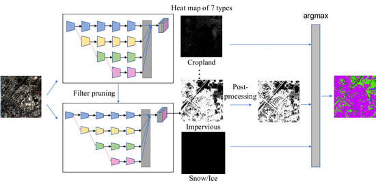
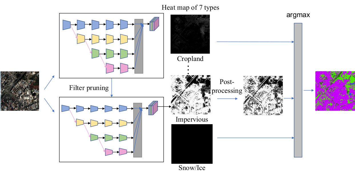
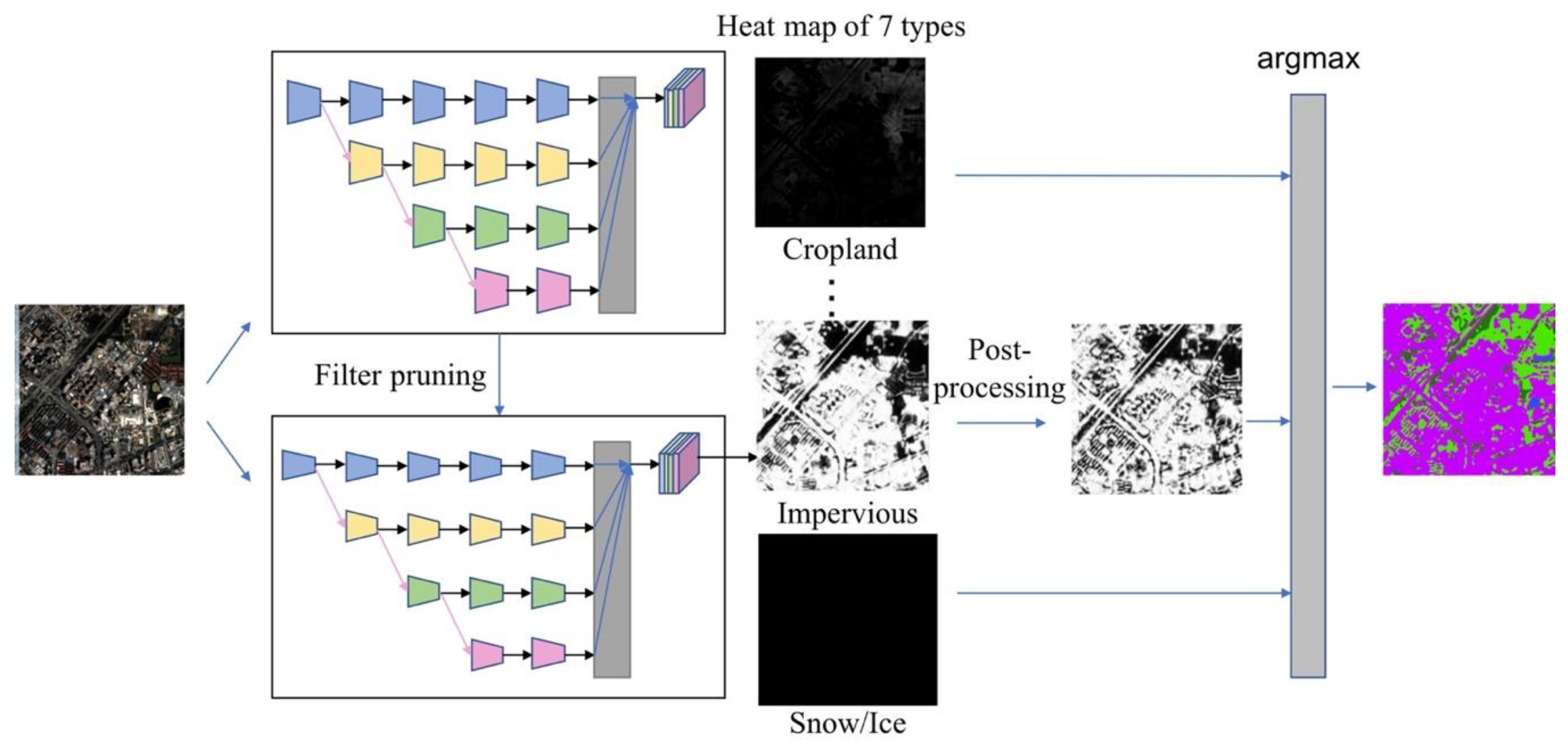
3.1. Overview of the Proposed Method

In this research, we propose a novel deep learning-based semantic segmentation approach to transform an imperfect 10-m resolution land cover product into preferable 3-m resolution land cover maps. The proposed approach integrates an improved high-resolution network (HRNet) with instance normalization, adaptive histogram equalization, and a pruning process that reduces the complexity and improves the efficiency of the model. Considering the dependence on the spatial information of high-resolution remote sensing applications, the improved HRNet can maintain strong high-resolution representations through keeping and fusing different resolution features, which will be described in more detail in Section 3.2.

To improve the generalization of our proposed approach, we replace the Batch Normalization (BN) [41] layer behind the first convolution layer with the Instance Normalization (IN), with more details shown in Section 3.2. In addition, we design a post-processing strategy with adaptive histogram equalization to improve the robustness of our proposed approach for the impervious type, which will be described in more detail in Section 3.3. It can effectively mitigate the problem that the road segmentation results (belonging to the impervious type) are always continuous, and the building segmentation results (belonging to the impervious type) are predicted in pieces without details.

To reduce the complexity and improve the efficiency of the model for the national-scale land cover mapping, we apply Filter Pruning via Geometric Median to compress the neural network based on the above resulting segmentation model. It can calculate the contribution of each filter to the network and remove the redundant filters with minor contribution. It is notable that we only use the pruned model for the inference in the large-scale land cover mapping. The overall workflow is shown in Figure 3.

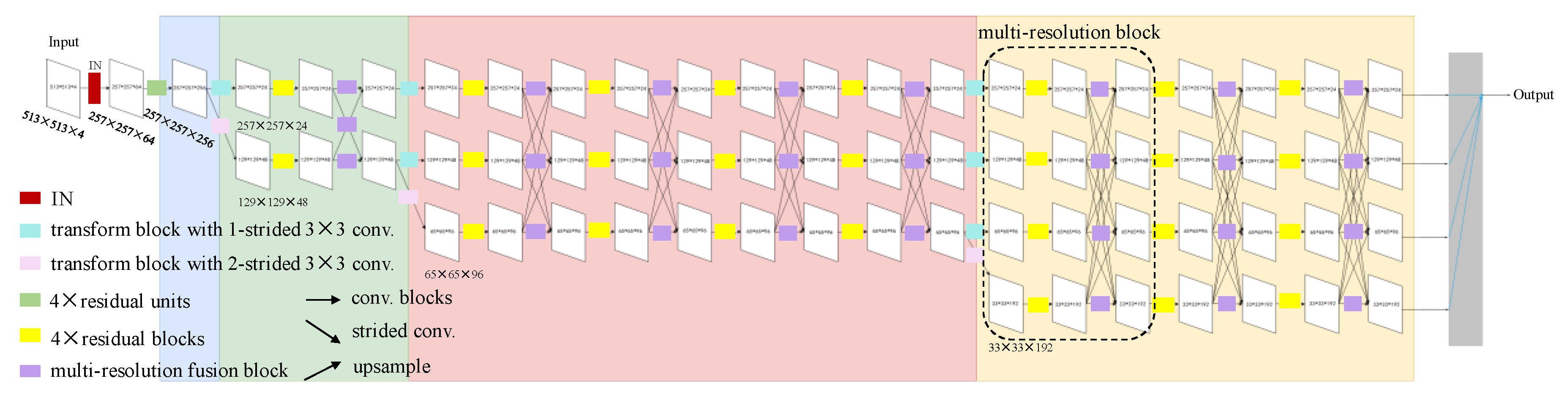
3.2. Neural Network Model

The commonly used segmentation models in recent land cover mapping studies, such as U-Net, use a decoder part and skip connection to recover high-resolution segmentation results from low-resolution representations, which are extracted from a high-to-low encoder part. The design of such a network can reasonably extract deep semantic features in the existing works. However, the encoder-decoder-based architecture may lose spatial details in the encoder part and introduce coarse features from shallow layers in the decoder part. Therefore, we implement a neural network model based on the high-resolution network (HRNet) [38] to maintain the rich high-level spatial information and repeatedly use the extracted deep semantic information. It can be divided into four stages, as represented by different colors of the background. Every branch denotes a different resolution, as represented by each row. Specifically, we down-sample the input image by a 2-strided 3 × 3 convolutional layer at first, which can effectively improve the efficiency without much image information loss. Then, the first stage contains 4 residual units (denoted by a green rectangle), and each unit is formed by a bottleneck module with a width of 64, the same as with the ResNet-50 [42]. In the transform block (denoted by a cyan rectangle), a horizontal arrow denotes a 1-strided 3 × 3 convolutional layer. An obliquely downward arrow in the transform block (denoted by a pink rectangle) denotes a 2-strided 3 × 3 convolutional layer, which transforms the input channels to 2 × input channels and down-samples the input. The second, third, and fourth stages contain 1, 4, and 3 multi-resolution blocks, respectively. A multi-resolution block (denoted by a black dotted box) is defined as the extraction and fusion of different resolution features. Each multi-resolution block consists of several single-resolution convolution blocks and a multi-resolution fusion block. A single-resolution convolution block (denoted by yellow rectangle) contains 4 residual blocks, each formed by two 3 × 3 convolutional layers. A multi-resolution fusion block (denoted by a purple rectangle) resembles the multi-branch fully-connection manner using up-sample and down-sample convolution layers. The transform blocks in the second, third, and fourth stages are similar to the first stage, and the only difference is the number of the output channels. The widths of the feature maps in the four stages are C, 2C, 4C, and 8C, respectively (C equals 24 in this paper). Finally, the merged output from the four different resolutions, which is rescaled through bilinear up-sampling, is resized to the same size with the input. The Softmax layer is applied to obtain the final segmentation map.

Due to the difference in acquisition time and image quality of satellite images, improving the generalization of our model can effectively reduce the potential errors caused by the variations in image qualities and increase the model robustness. In general, Batch Normalization (BN), calculating the mean and variance of each batch of training data, is applied in deep learning networks to normalize the data distribution for the stabilized training. However, facing the highly-possible variations in data quality in the original satellite images, Instance Normalization (IN) is more suitable. IN calculates the mean and variance of each single image rather than of the images of each batch, reducing the dependency on image quality. Therefore, we make a simple yet effective modification by replacing the BN layer behind the first convolution layer with the IN, which can effectively increase the generalization of the model. In addition, in order to solve the problem of sample imbalance, for the impervious type with relatively small proportion and complex targets (such as road and building), increasing the corresponding weight in the loss function (i.e., cross entropy loss) can effectively improve the detection of this type and improve the training efficiency and precision.

The architecture of the neural network is shown in Figure 4. The size of the input image is 513 × 513 pixels, which is an empirically optimal size considering the receptive field and GPU memory. We empirically improve the weight of the impervious type to 3 in the loss function. We train our model for 120 epochs with a total batch size of 32 using the Pytorch framework, with the job processed in parallel by 16 GPUs. The initial learning rate is set to 0.01 and a stochastic gradient descent (SGD) is applied with a momentum of 0.9.

3.3. Contrast Limited Adaptive Histogram Equalization Post-Processing

Impervious is an important yet imbalanced and indistinguishable type in our study. As the supervised label generated from the 10-m resolution land cover product is relatively coarse in the city area with many mixed types, the road (belonging to Impervious) segmentation results are not always continuous, and the building (belonging to Impervious) segmentation results are predicted in pieces without details. Therefore, contrast limited adaptive histogram equalization (CLAHE) [43] is applied to enhance the local contrast of the impervious type for stronger discrimination. The adaptive method redistributes the lightness values of the image based on several histograms, each histogram corresponding to a different portion of the image. The size of the block processed each time is set to 512 × 512 in a predicted image with a size of 8000 × 8000, which is an experimental best size in large-scale land cover mapping.

In the specific implementation, first, we extract the probability map of impervious type after the Softmax layer. The probability map is mapped from [0, 1] to [0, 255] so that the CLAHE can be applied. After the CLAHE processing, the prediction mask of impervious type can be obtained by setting a threshold. We use the impervious mask to weight the original probability values. The probability value is doubled, where the value is positive on the impervious mask. Otherwise, the probability value is halved. Note that only the probability values of impervious type are weighted and the values of other types are not changed. Finally, the prediction results can be obtained by the Argmax function.

3.4. Filter Pruning for Feature Dimension Reduction and Neural Network Acceleration

To reduce the model storage space and speed up the inference in large-scale land cover mapping, we apply Filter Pruning via Geometric Median (FPGM) [44] to the modified HRNet obtained in Section 3.2. It compresses the neural network by pruning redundant filters, and the process is summarized in Algorithm 1. The HRNet model trained in Section 3.2 is used as the pre-trained model. He et al. applied FPGM for VGG and ResNet as examples [44], while the architecture of our modified HRNet is more complex, with increased multi-resolution feature fusions. Therefore, all the convolutional layers of the model, except for the latest layers before the multi-resolution fusion block, are pruned by a ratio of 40%. The main idea of the FPGM is that if some filters are the same or similar to the other filters in the same layer, these filters can be represented by the other filters and cropped without a great influence on the model performance. Specifically, we calculate the sum of the 2-norms of each filter with the other filters in the same layer, sort the sums from small to large, and set the parameters of the first 40% filters to zero. We perform the pruning in such a way because the smaller values indicate that they are more similar to other filters, as shown in Equation (1):

$$F_{i,j^{*}}\in \underset{j^{*}\in \left[1, N_i\right]}{\mathrm{argmin}}{\displaystyle \sum }_{j^{\prime }\in \left[1, N_i\right]}||x-F_{i,j^{\prime }}|{|}_2$$

(1)

where $F_{i,j^{*}}$ are the filters needing to be pruned, which represent several jth filters in the ith layer. We use $N_i$ to represent the number of the filters of the ith layer.

Then, the pruned model parameters are updated to the previous model as the pre-trained model in the next training epoch. The model is continuously trained in a regular way, and we repeat the above pruning process until the end of the iteration. Finally, the compact model is obtained by deleting the filters with zero.

Algorithm 1. Algorithm Description of FPGM

Input: training data: X.

1: Given: pruning rate 40%

2: Initialize: model parameter $W=\left\{W^{\left(i\right)}, 0\le i\le L\right\}$

3: for epoch = 1; $\mathrm{epoch} \le {\mathrm{epoch}}_{max};\mathrm{epoch} ++$ do

4:   Update the model parameter W based on X

5:   for $i=1; i\le L; i++$ do

6:     Find $40\% \times N_i$ filters that satisfy Equation (1)

7:     Zeroize selected filters

8:   end for

9: end for

10: Obtain the compact model $W^{*}$ from $W$

Output: The compact model and its parameters $W^{*}$

4. Experimental Results

4.1. The Quantitative Results of the 3-m Resolution Land Cover Maps of China

In this section, we quantify the 3-m resolution land cover mapping results and compare them with their 10-m resolution counterparts on the test dataset in China. The 10-m resolution land cover mapping results are from the public product for 2017 [4]. We matched the corresponding coordinate points to get 10-m resolution classification results.

Table 2. The confusion matrix obtained from the 10-m resolution land cover product in China.

Name	Cropland	Woodland	Grassland	Water	Impervious	Bare Land	Snow/Ice	SUM	UA (%)
Cropland	263	34	32	3	36	1	0	369	71.27
Woodland	27	373	30	0	2	0	0	432	86.34
Grassland	32	17	188	1	12	32	0	282	66.67
Water	0	3	1	89	1	3	2	99	89.90
Impervious	9	1	2	2	132	1	0	147	89.80
Bare land	5	9	49	2	8	526	3	602	87.38
Snow/Ice	0	0	1	0	0	3	5	9	55.56
SUM	336	437	303	97	191	566	10	1940
PA (%)	78.27	85.35	62.05	91.75	69.11	92.93	50.00		81.24 *

* The value denotes the Overall Accuracy (OA).

and

Table 3. The confusion matrix obtained from the 3-m resolution land cover product in China.

Name	Cropland	Woodland	Grassland	Water	Impervious	Bare Land	Snow/Ice	SUM	UA (%)
Cropland	282	27	20	3	20	1	0	353	79.89
Woodland	21	391	26	2	6	0	1	447	87.47
Grassland	22	10	223	1	7	19	0	282	79.08
Water	1	1	0	84	2	2	0	90	93.33
Impervious	8	1	2	4	150	2	0	167	89.82
Bare land	2	7	32	3	6	542	6	598	90.64
Snow/Ice	0	0	0	0	0	0	3	3	100.00
SUM	336	437	303	97	191	566	10	1940
PA (%)	83.93	89.47	73.60	86.60	78.53	95.76	30.00		86.34 *

* The value denotes the Overall Accuracy (OA).

show the confusion matrices derived from the 10-m resolution map and the 3-m resolution test sample set, respectively.

The User’s Accuracy (UA) is the fraction of retrieved instances that are relevant, and the Producer’s Accuracy (PA) is the fraction of relevant instances that are retrieved [45]. We also calculate the Overall Accuracy (OA), which represents the number of correctly classified sample sets divided by the total number of sample units [46]. The overall accuracies of the 10-m resolution map and the 3-m resolution test sample set are 81.24% and 86.34%. The transformed 3-m resolution land cover classification result using our proposed approach improved the OA by 5.1% from the 10-m resolution land cover mapping result. For the types of cropland, woodland, grassland, impervious and bare land, the 3-m resolution land cover maps improved the PA by 5.65%, 4.12%, 11.55%, 9.42%, and 2.83%, respectively, compared to the 10-m resolution land cover maps, benefitting from the high-resolution satellite image and the full use of the spatial information in the 3-m data. The PA of the water type declined from 91.75% (10-m resolution) to 86.60% (3-m resolution). We think that this is largely due to there being fewer bands in the 3-m resolution image. The spectrum features, as demonstrated in previous work [45], can play a big role in determining the water bodies. However, if we look at the UA for the water type, our approach with 3-m resolution data improves the result from 89.90% (10-m resolution) to 93.33% (3-m resolution). The better UA for the water type demonstrates that the extra spatial information can effectively help remove the false detection results (more detailed discussion is given in Section 4.2). The results of the snow/ice type are similar to those of the water type (more detailed discussion is given in Section 5.4).

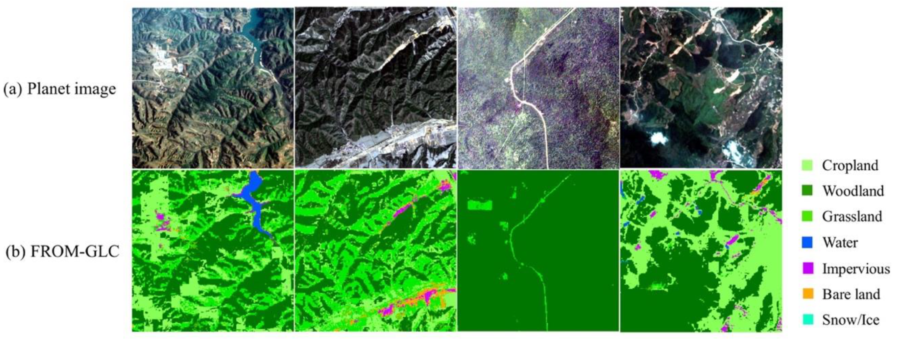
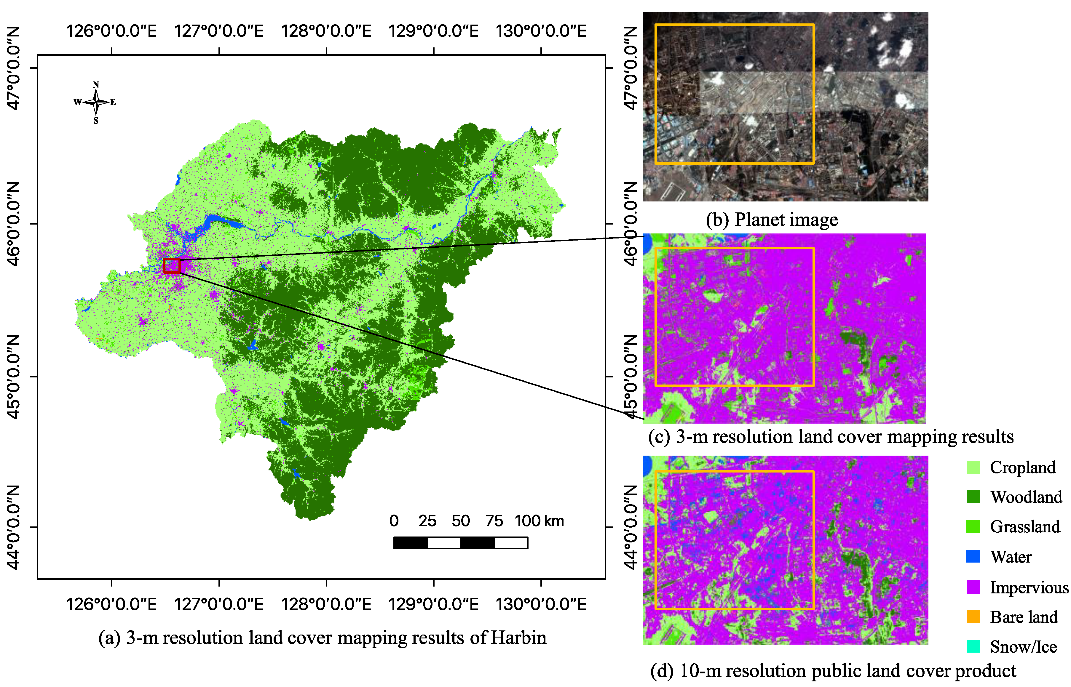
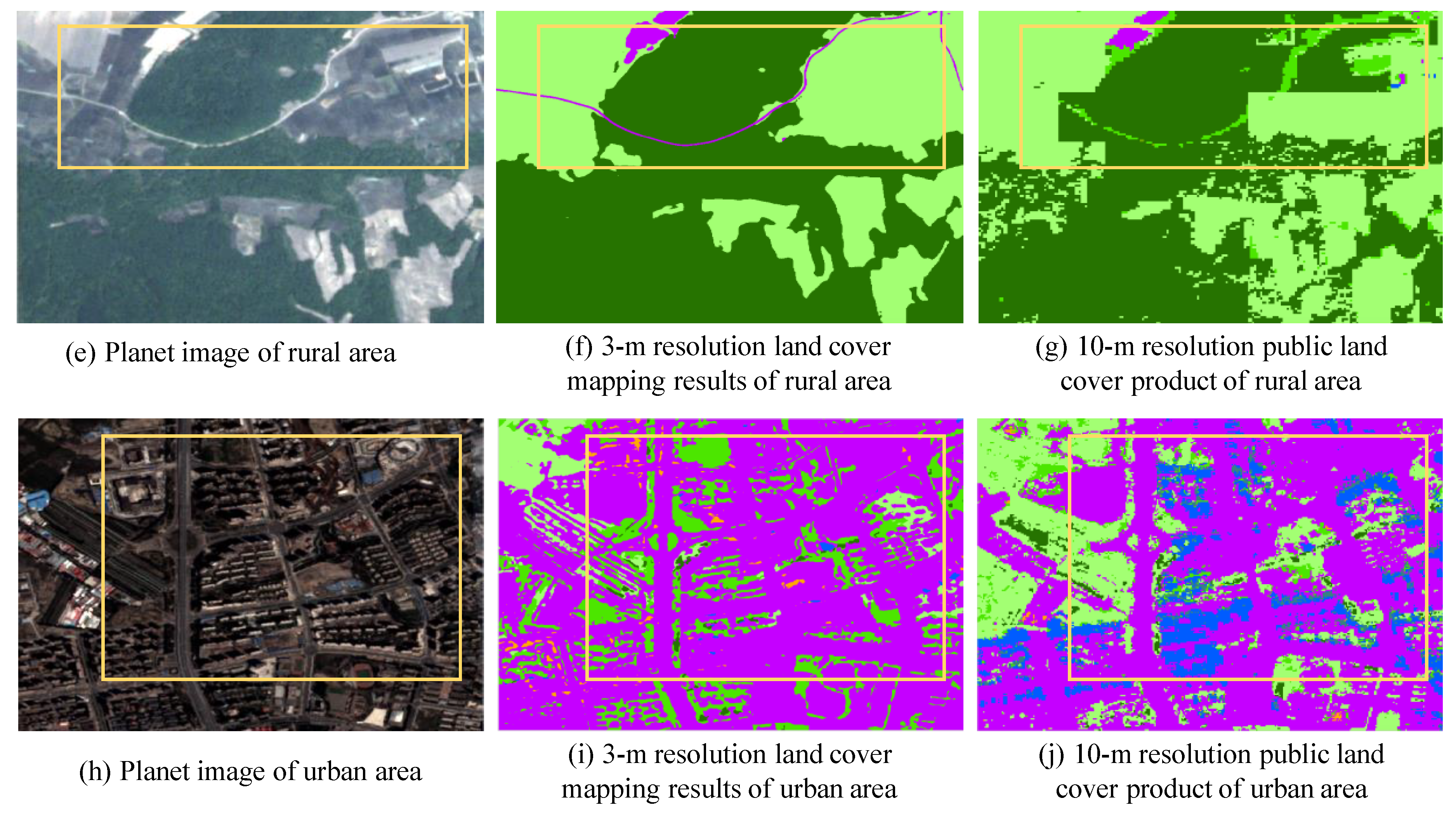
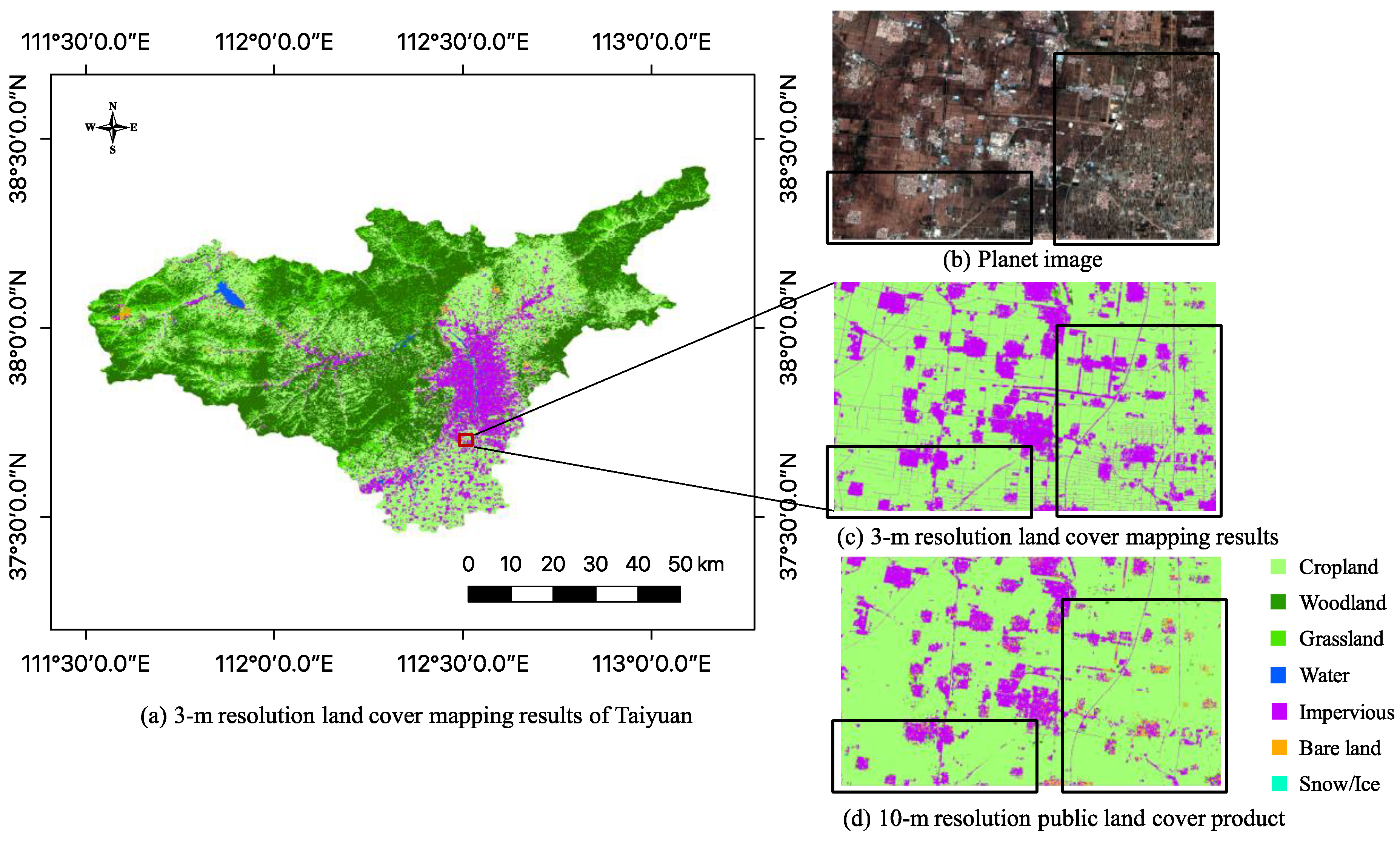
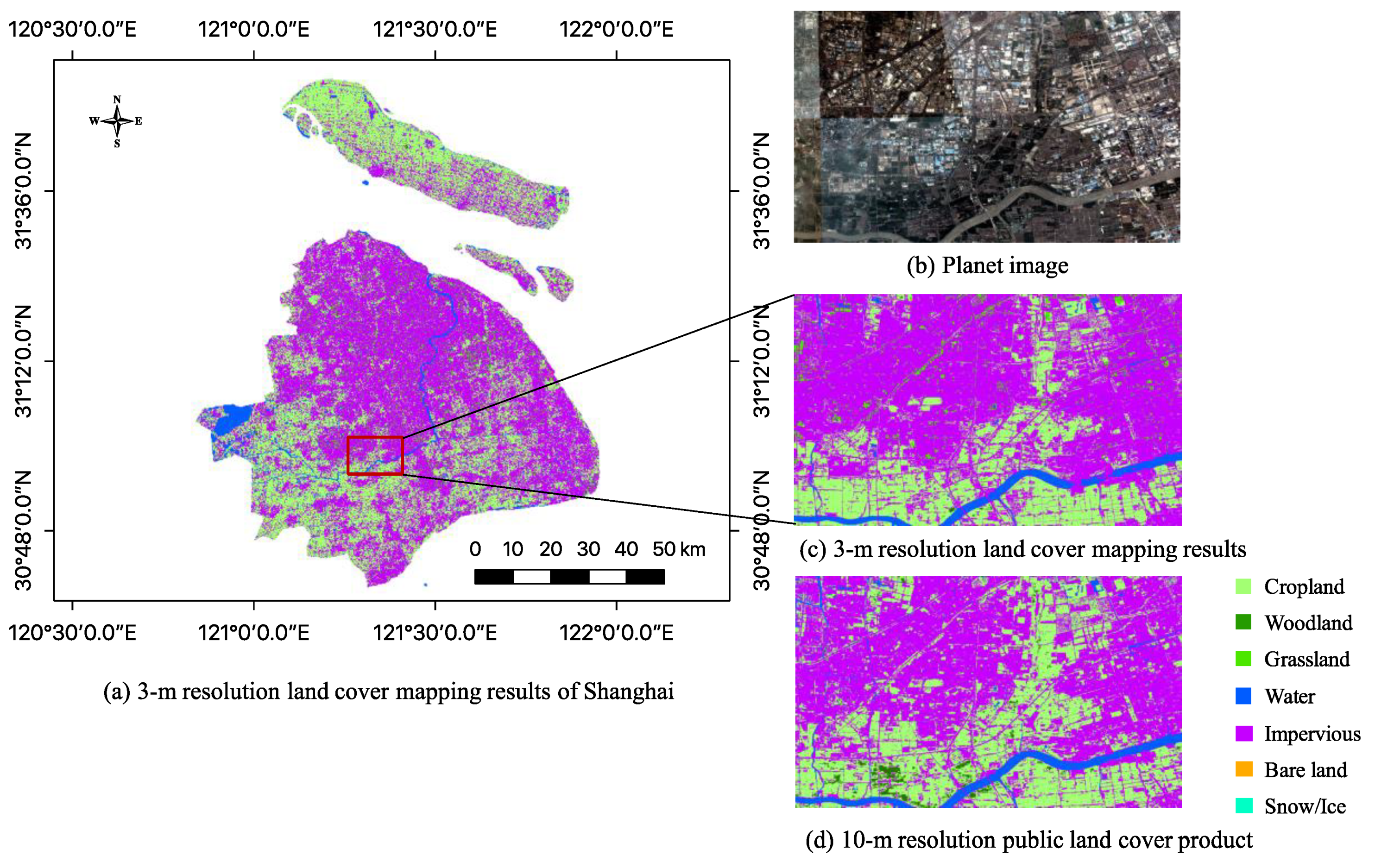
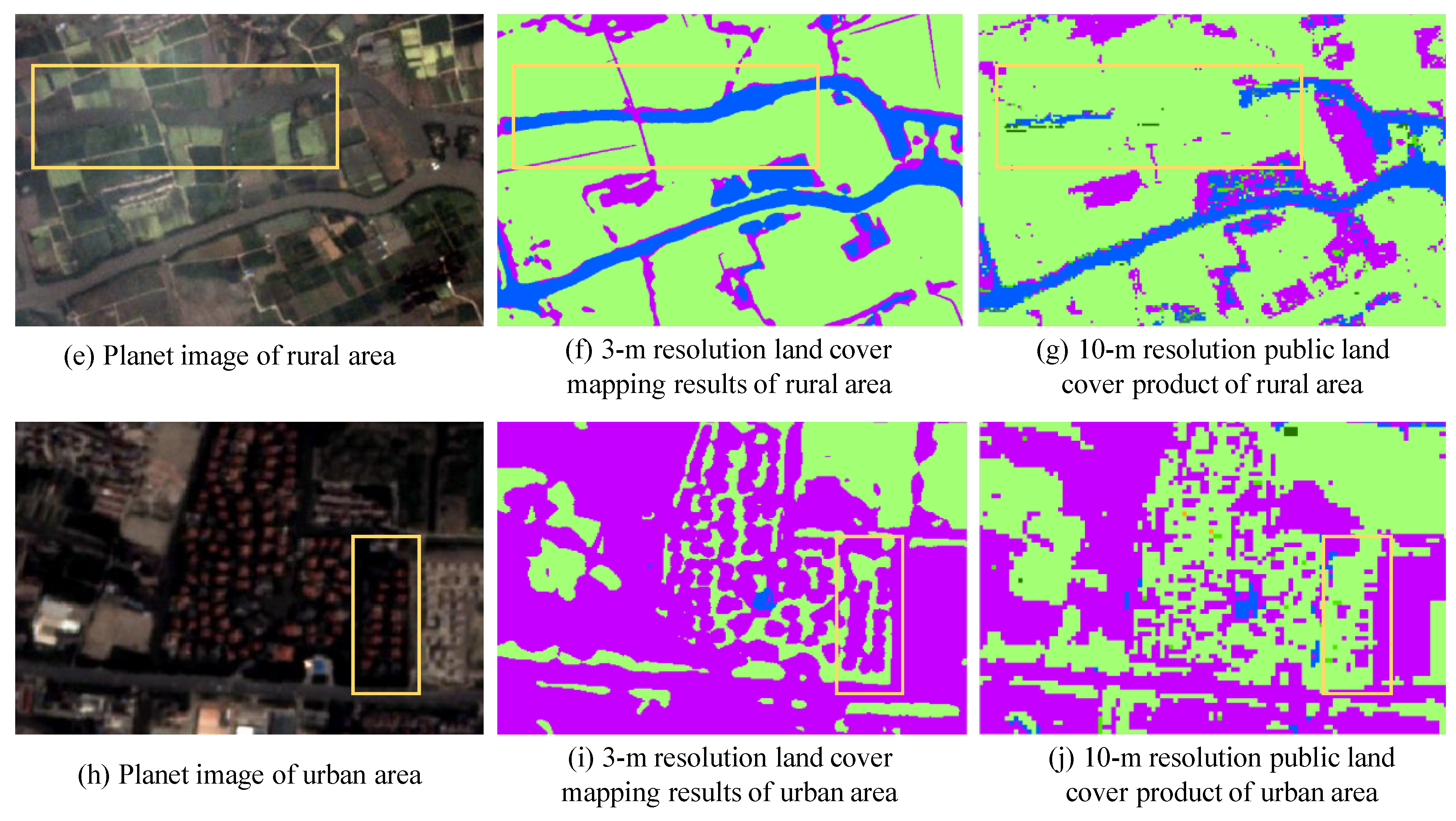
4.2. Examples of Land Cover Mapping in China

To evaluate the effectiveness of our proposed approach for large-scale land cover mapping, we present the 3-m resolution land cover maps over three mega cities in China (i.e., Harbin, Taiyuan, and Shanghai). These three cities represent different characteristics of landforms in China. The detailed comparison results of 3-m resolution and 10-m resolution land cover products are shown for both rural and urban areas. We analyze the comparison results through Figure 5, Figure 6 and Figure 7. In general, owning to the effective extraction of spatial information, our proposed method can reduce the incorrect pixel predictions in the 10-m resolution land cover map caused by the pixel-based classification method. From Figure 5e–j, and Figure 6e–g, we can see that Cropland tends to be confused with Woodland in FROM-GLC10, while our proposed approach can effectively reduce the confusion and hence obtain higher accuracies for these two types. From Figure 5b–d, Figure 5h–j, and Figure 7h–j, the impervious classification results of FROM-GLC10 tend to be underestimated. Our proposed approach reduces the confusion between Impervious and Water, and obtains more accurate impervious segmentation results compared with FROM-GLC10. In addition, owing to the higher resolution satellite image and the post-processing, our proposed method can better capture linear and small objectives (e.g., road and narrow river). The road segmentation results (belonging to the impervious type) have clearly outperformed FROM-GLC10, as shown by Figure 5e–j, Figure 6b–d, and Figure 6h–j. Figure 7e–g show the improved capturing of narrow river (belonging to the water type). Consequently, our proposed approach achieves an effective improvement of transferring the imperfect 10-m resolution land cover maps to the 3-m finer resolution land cover maps in China.

5. Discussion

5.1. Analysis of Accuracies between 3-m and 10-m Resolution Land Cover Maps

We analyze the reliability of the accuracy comparison between the 3-m and 10-m resolution land cover maps. First, we discuss the construction of the test dataset with seven types, based on the test dataset with ten types [1]. According to the definition of Woodland in our classification system, we combined the results of Forest and Shrubland and use the sample units of those two types for the accuracy calculation for Woodland in the 10-m resolution land cover map. As the numbers of Tundra and Wetland sample units were only 1 and 26 in China, the removal of these two types of sample unit would not have much impact on the accuracy comparison. It should be noted that we only compare the seven types in common. In addition, as the number of original sample units of Water and Impervious is only 18 and 50 in China, we supplemented sample units for these two types for more reliable accuracy assessment.

We also further discuss the impact of original product accuracy and resolution on the high-resolution land cover mapping. We assume that excessive resolution differences (e.g., more than 10 times) between products and high-resolution images are not suitable for supervised deep learning methods. By contrast, it can be regarded as a weakly supervised learning problem as defined in [22]. However, more accurate products could help more effective learning, but the improvement also depends on the amount of information contained in the high-resolution images.

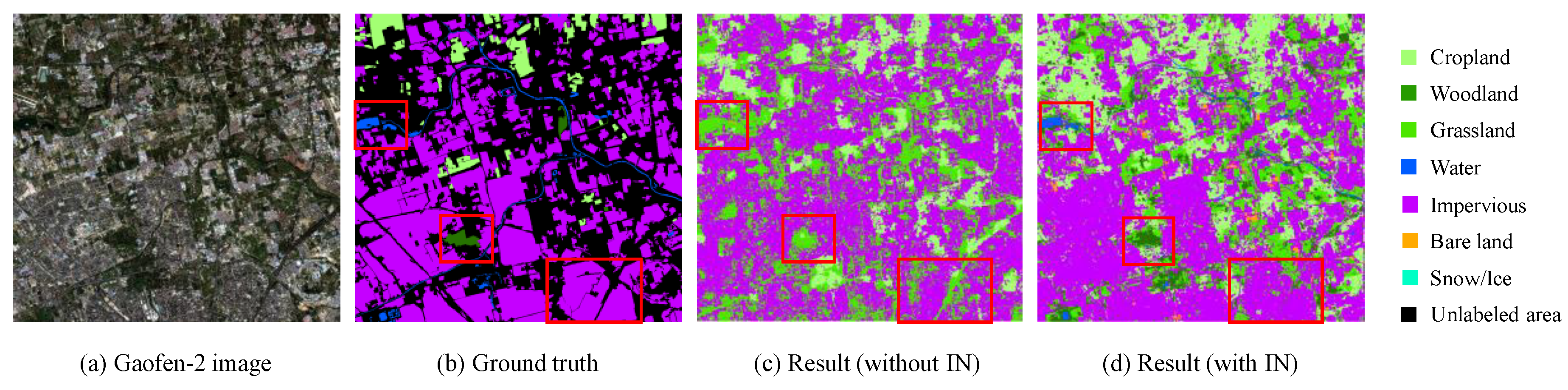
5.2. The Effectiveness of Our Proposed Network and Post-Processing

In this section, we analyze the effectiveness of the network (introduced in Section 3.2) and the post-processing (introduced in Section 3.3) in this application. First of all, we compare the high-resolution network (HRNet) with commonly used and stable CNN architectures in the deep learning domain (e.g., fully convolutional densenet (FC-DenseNet) and U-Net). The comparison experiments use the same dataset and the same set of strategies for pre-processing, training (such as the learning rate and the number of GPUs), and post-processing. All models have been fully trained and converged for valid comparison. The FC-DenseNet64 is implemented following [47] and the U-Net is implemented following [48]. The maximum receiving field sizes of U-Net, FC-Densenet64, and HR-Net (in this work) are 130 × 130, 695 × 695, and 1439 × 1439, respectively. Note that due to the padding process, the actual receptive field is lower than the theoretical value. The comparison results are shown in

Table 4. Comparison results for the test dataset between the high-resolution network and other CNN architectures (i.e., FC-Densenet and U-Net).

Models	PA (%)							OA (%)
	Cropland	Woodland	Grassland	Water	Impervious	Bare Land	Snow/Ice
10-m resolution map	78.27	85.35	62.05	91.75 *	69.11	92.93	50.00 *	81.24
U-Net	73.21	88.79	70.96	86.60	75.92	95.05	20.00	83.40
FC-DenseNet	81.55	91.08 *	68.32	84.54	68.59	94.52	0.00	83.87
HRNet (ours)	83.93 *	89.47	73.60 *	86.60	78.53 *	95.76 *	30.00	86.34 *

* The values denote the best results.

. The high-resolution network outperforms FC-DenseNet and U-Net by 2.47% and 2.94% in OA, respectively, owing to the maintenance of strong high-resolution representations and the combination of different resolution representations by our network. Therefore, we can conclude that the high-resolution network is more suitable for this task.

The generalization and robustness of the model is important for remote sensing applications, especially when facing images with a wide variety of sensor and image qualities. In our approach, the instance normalization part is an important module for achieving that. To better identify the generalization and robustness of our model, we test images from different satellite sources. We show an example from the Gaofen Image Dataset (GID) [16] to analyze the effectiveness of our Instance Normalization (IN) module. The image in Figure 8a was acquired from the Gaofen-2 satellite at a 4-m resolution with a size of 7200 × 6800 pixels. The classification system of the GID contains five major types (e.g., Farmland, Forest, Meadow, Water, and Built-up), which substantially match five types (e.g., Cropland, Woodland, Grassland, Water, Impervious) in our classification system. We train another model without IN for comparison. Note thatthe models are trained on the dataset described in Section 2.3 and that the GID data are only for testing. The comparison results are shown in Figure 8. From the red rectangles, the result of the model with IN is significantly better than the result of the model without IN, as the former can effectively reduce confusion among different types. The usage of IN does not bring the accuracy improvement with our test dataset, as the images in our test dataset were acquired from the same satellite sensor and within a similar time frame. However, when applying our model to land cover mapping for large-scale areas in different years, the generalization and robustness of the model with IN can effectively reduce the errors caused by the variations in image quality and satellite source.

A significant improvement in road extraction (belonging to the impervious type) is obtained in large-scale land cover mapping through the post-processing, and urban areas benefit more from this strategy. We show an example in Figure 9. The left red rectangle in Figure 9a represents a dense impervious area, and the rectangle on the right represents a sparse impervious area. It can be found that different responses exist between the dense impervious area and the sparse impervious area in Figure 9b. By analyzing the heat map of this type, it is found that the response is higher in the dense impervious area, while it is lower in the sparse impervious area. The responses are not distinguishable enough between the impervious type and other land cover types, which causes road (belonging to the impervious type) prediction results to be discontinuous and the vegetation between buildings to be difficult to identify. As shown in Figure 9c, the responses are almost consistent both in the dense impervious area and in the sparse impervious area from the post-processing, and more distinguishable between impervious and other land cover types. Note that the post-processing strategy provides more spatial details for the impervious type, although the overall accuracy is the same as for the results without the post-processing strategy.

5.3. The Computational Efficiency of Our Proposed Method in Large-Scale Land Cover Mapping

In order to make it possible to produce the China land cover map, we apply filter pruning for network compression and acceleration with almost no loss of accuracy. The specific overall accuracy, reduced parameters, and theoretical acceleration in our proposed network are shown in

Table 5. Comparison of the baseline model and the pruned model in terms of overall accuracy, number of parameters, model size, and theoretical acceleration.

Models	Overall Accuracy (%)	Number of Parameters	Model Size (MB)	Theoretical Acceleration (%)
Baseline model	86.34	16,812,946	130	-
Pruned model	86.04	9,720,660	39	52.63

. The realistic acceleration varies from different deep learning platforms. Non-tensor layers, such as batch normalization (BN), are not pruned and still need the inference time on the GPU, which influences the realistic acceleration. In addition, the IO delay and efficiency of BLAS libraries also influence the realistic acceleration. In this work, it takes about 1.2 s to predict two 1024 × 1024 images on a single GPU using two prediction tasks. Therefore, taking into account the overhead of overlapping predictions, the entire China land cover model inference could be done in 5 h on 64 GPU cards. Note that our best model reaches 86.34% OA for China. The pruned model achieves a slightly lower OA of 86.04%, but provides the option to process the images of the whole of China in a more efficient way.

5.4. Shortcomings with 3-m Resolution Land Cover Map and Potential Strategies for Further Research

The first issue is the slight traces of stitching in large-scale land cover mapping. Due to the inconsistent acquisition date of each image tile, there are slight radiation differences between Planet image tiles, as shown in Figure 5b and Figure 7b. We applied Instance Normalization (IN) in the network to normalize the extracted features by calculating the mean and variance of each single image. Although this can reduce the dependency on image quality and hence reduce the traces of stitching, the land cover maps could still be further improved by carefully integrating Instance Normalization (IN) and Batch Normalization (BN) to improve the generalization capacity of the network.

The second issue is that the results of water and snow/ice types in the 3-m resolution land cover maps are not effectively improved. This results from the limited spectral information of the 3-m resolution data (with four bands) compared with the 10-m resolution data (with ten bands). It has a huge negative impact on the identification of water and snow/ice types, which greatly benefits from spectral information. Multi-source data fusion is a potential strategy. The 3-m resolution land cover mapping results could be further improved if 10-m resolution satellite images with rich spectral and temporal information were utilized in our proposed method. In addition, as the satellite images are acquired in summer, there are only a few sample units of the snow/ice type and the prediction results for this type are less than normal. These issues should be addressed in future research.

The third issue concerns the cloud coverage of single temporal image. Cloud coverage has a greater impact on the land cover mapping results, even though we have selected the images with the least cloud coverage. These issues should be improved by using multi-temporal images in future research.

The fourth issue is related to the level of thematic detail that could be further expanded with 3-m resolution data. In future work, more detailed land cover types will be experimented with to take advantage of the high spatial resolution of the data and the better use of spatial contexts offered by the deep-learning algorithms.

6. Conclusions

In this paper, we transfer 10-m resolution land cover mapping results to 3-m resolution land cover mapping for China. We have explored a possible solution for completing this work without human efforts. With our proposed land cover mapping approach, a higher accuracy than with the 10-m land cover data is obtained by 3-m land cover classification owing to the robust deep learning based neural network with maintained high-resolution representation. We further adopt Instance Normalization (IN) after the first convolution layer to improve the generalization and robustness of the model. More spatial details of the impervious type are obtained owing to the post-processing strategy, which fully utilizes the heat maps obtained from the neural network and greatly reduces the impact of the coarse supervised labels generated by the 10-m resolution data. More efficient inference is obtained owing to the compressed model by filter pruning via geometric median. Therefore, we can effectively and efficiently obtain a more promising 3-m resolution land cover map (an improvement of 5.1% in OA over the 10-m resolution land cover product) should similar 3-m resolution satellite images be used to map the whole of China. Our approach demonstrates the possibility of scaling from existing lower resolution mapping products to higher resolution mapping products and can significantly reduce the cost and human efforts required for performing such large-scale mapping projects. In future research, we will further improve the robustness of our proposed approach in the presence of noisy labels. We will also explore the combination of other open data sources (e.g., OSM) for building a better training dataset.

References

1. Gong, P.; Wang, J.; Yu, L.; Zhao, Y.; Zhao, Y.; Liang, L.; Niu, Z.; Huang, X.; Fu, H.; Liu, S.; et al. Finer resolution observation and monitoring of global land cover: First mapping results with Landsat TM and ETM+ data. Int. J. Remote Sens. 2013, 34, 2607–2654. [Google Scholar] [CrossRef] [Green Version]
2. Robinson, C.; Hou, L.; Malkin, K.; Soobitsky, R.; Czawlytko, J.; Dilkina, B.; Jojic, N. Large Scale High-Resolution Land Cover Mapping with Multi-Resolution Data. In Proceedings of the IEEE Conference on CVPR, Long Beach, CA, USA, 16–20 June 2019; pp. 12726–12735. [Google Scholar]
3. Tong, X.; Zhao, W.; Xing, J.; Fu, W. Status and development of China High-Resolution Earth Observation System and application. In Proceedings of the IEEE International Geoscience and Remote Sensing Symposium, Beijing, China, 10–15 July 2016. [Google Scholar]
4. Gong, P.; Liu, H.; Zhang, M.; Li, C.; Wang, J.; Huang, H.; Clinton, N.; Ji, L.; Li, W.; Bai, Y.; et al. Stable classification with limited sample: Transferring a 30-m resolution sample set collected in 2015 to mapping 10-m resolution global land cover in 2017. Sci. Bull. 2019, 64, 370–373. [Google Scholar] [CrossRef] [Green Version]
5. Hansen, M.; DeFries, R.; Townshend, J.; Sohlberg, R. Global land cover classification at 1 km spatial resolution using a classification tree approach. Int. J. Remote Sens. 2000, 21, 1331–1364. [Google Scholar] [CrossRef]
6. Loveland, T.R.; Reed, B.C.; Brown, J.F.; Ohlen, D.O.; Zhu, Z.; Yang, L.; Merchant, J.W. Development of a global land cover characteristics database and igbp discover from 1 km avhrr data. Int. J. Remote Sens. 2000, 21, 1303–1330. [Google Scholar] [CrossRef]
7. Friedl, M.; Sulla-Menashe, D.; Tan, B.; Schneider, A.; Ramankutty, N.; Sibley, A.; Huang, X. Modis collection 5 global land cover: Algorithm refinements and characterization of new datasets. Remote Sens. Environ. 2010, 114, 168–182. [Google Scholar] [CrossRef]
8. Sulla-Menashe, D.; Gray, J.M.; Abercrombie, S.P.; & Friedl, M.A. Hierarchical mapping of annual global land cover 2001 to present: The modis collection 6 land cover product. Remote Sens. Environ. 2019, 222, 183–194. [Google Scholar] [CrossRef]
9. Arino, O.; Bicheron, P.; Achard, F.; Latham, J.; Witt, R.; Weber, J.-L. GLOBCOVER: The most detailed portrait of Earth. Eur. Space Agency Bull. 2008, 136, 25–31. [Google Scholar]
10. Bontemps, S.; Defourny, P.; Van Bogaert, E.; Arino, O.; Kalogirou, V.; Perez, J.R. GLOBCOVER 2009 Products Description and Validation Report. 2011. Available online: http://ionia1.esrin.esa.int/docs/GLOBCOVER2009_Validation_Report_2,2 (accessed on 30 April 2018).
11. Land Cover CCI: Product User Guide Version 2.0. 2017. Available online: www.esa-landcover-cci.org (accessed on 30 April 2018).
12. Ma, L.; Li, M.; Ma, X.; Cheng, L.; Du, P.; Liu, Y. A review of supervised object-based land-cover image classification. ISPRS J. Photogramm. 2017, 130, 277–293. [Google Scholar] [CrossRef]
13. Zhang, C.; Sargent, I.; Pan, X.; Li, H.; Gardiner, A.; Hare, J.; Atkinson, P.M. Joint Deep Learning for land cover and land use classification. Remote Sens. Environ. 2019, 221, 173–187. [Google Scholar] [CrossRef] [Green Version]
14. Ma, L.; Liu, Y.; Zhang, X.; Ye, Y.; Yin, G.; Johnson, B.A. Deep learning in remote sensing applications: A meta-analysis and review. ISPRS J. Photogramm. 2019, 152, 166–177. [Google Scholar] [CrossRef]
15. Deng, J.; Dong, W.; Socher, R.; Li, L.J.; Li, K.; Li, F. Imagenet: A large-scale hierarchical image database. In Proceedings of the IEEE Conference on CVPR, Miami, FL, USA, 20–26 June 2009; pp. 248–255. [Google Scholar]
16. Tong, X.; Xia, G.; Lu, Q.; Shen, H.; Li, S.; You, S.; Zhang, L. Learning Transferable Deep Models for Land-Use Classification with High-Resolution Remote Sensing Images. arXiv 2018, arXiv:1807.05713. [Google Scholar]
17. Demir, I.; Koperski, K.; Lindenbaum, D.; Pang, G.; Huang, J.; Basu, S.; Raska, R. Deepglobe 2018: A challenge to parse the earth through satellite images. In Proceedings of the IEEE Conference on CVPRW, Salt Lake City, UT, USA, 18–22 June 2018; pp. 172–17209. [Google Scholar]
18. Zhang, H.K.; Roy, D.P. Using the 500 m MODIS land cover product to derive a consistent continental scale 30 m Landsat land cover classification. Remote Sens. Environ. 2017, 197, 15–34. [Google Scholar] [CrossRef]
19. Lee, J.; Cardille, J.A.; Coe, M.T. BULC-U: Sharpening Resolution and Improving Accuracy of Land-Use/Land-Cover Classifications in Google Earth Engine. Remote Sens. 2018, 10, 1455. [Google Scholar] [CrossRef] [Green Version]
20. Zhang, X.; Liu, L.; Wang, Y.; Hu, Y.; Zhang, B. A SPECLib-based operational classification approach: A preliminary test on China land cover mapping at 30 m. Int. J. Appl. Earth Obs. Geoinfor. 2018, 71, 83–94. [Google Scholar] [CrossRef]
21. Schmitt, M.; Hughes, H.L.; Qiu, C.; Zhu, X.X. SEN12MS–A Curated Dataset of Georeferenced Multi-Spectral Sentinel-1/2 Imagery for Deep Learning and Data Fusion. arXiv 2019, arXiv:1906.07789. [Google Scholar] [CrossRef] [Green Version]
22. Schmitt, M.; Prexl, J.; Ebel, P.; Liebel, L.; Zhu, X.X. Weakly supervised semantic segmentation of satellite images for land cover mapping–challenges and opportunities. arXiv 2020, arXiv:2002.08254. [Google Scholar]
23. Kaiser, P.; Wegner, J.; Lucchi, A.; Jaggi, M.; Hofmann, T.; Schindler, K. Learning aerial image segmentation from online maps. IEEE Trans. Geosci. Remote Sens. 2017, 55, 6054–6068. [Google Scholar] [CrossRef]
24. Gong, P.; Chen, B.; Li, X.; Liu, H.; Wang, J.; Bai, Y.; Chen, J.; Chen, X.; Fang, L.; Feng, S.; et al. Mapping essential urban land use categories in China (EULUC-China): Preliminary results for 2018. Sci. Bull. 2020, 65, 182–187. [Google Scholar] [CrossRef] [Green Version]
25. Ren, M.; Zeng, W.; Yang, B.; Urtasun, R. Learning to reweight examples for robust deep learning. arXiv 2018, arXiv:1803.09050. [Google Scholar]
26. Kim, Y.; Yim, J.; Yun, J.; Kim, J. Nlnl: Negative learning for noisy labels. In Proceedings of the IEEE Conference on CVPR, Long Beach, CA, USA, 16–20 June 2019; pp. 101–110. [Google Scholar]
27. Dong, R.; Li, W.; Fu, H.; Gan, L.; Yu, L.; Zheng, J.; Xia, M. Oil palm plantation mapping from high-resolution remote sensing images using deep learning. Int. J. Remote Sens. 2019, 41, 2022–2046. [Google Scholar] [CrossRef]
28. Audebert, N.; Le Saux, B.; Lefèvre, S. Semantic segmentation of earth observation data using multimodal and multi-scale deep networks. In Proceedings of the Asian Conference on Computer Vision, Taipei, Taiwan, 20–24 November 2016; pp. 180–196. [Google Scholar]
29. Liu, Z.; Mu, H.; Zhang, X.; Guo, Z.; Yang, X.; Cheng, T.K.T.; Sun, J. MetaPruning: Meta Learning for Automatic Neural Network Channel Pruning. arXiv 2019, arXiv:1903.10258. [Google Scholar]
30. Zhao, H.; Shi, J.; Qi, X.; Wang, X.; Jia, J. Pyramid scene parsing network. In Proceedings of the IEEE Conference on CVPR, Honolulu, HI, USA, 21–26 July 2017; pp. 2881–2890. [Google Scholar]
31. Lin, G.; Milan, A.; Shen, C.; Reid, I. Refinenet: Multi-path refinement networks for high-resolution semantic segmentation. In Proceedings of the IEEE Conference on CVPR, Honolulu, HI, USA, 21–26 July 2017; pp. 1925–1934. [Google Scholar]
32. Zhuang, B.; Shen, C.; Tan, M.; Liu, L.; Reid, I. Towards effective low-bitwidth convolutional neural networks. In Proceedings of the IEEE Conference on CVPR, Salt Lack City, UT, USA, 18–22 June 2018; pp. 7920–7928. [Google Scholar]
33. Chen, Y.; Fan, H.; Xu, B.; Yan, Z.; Kalantidis, Y.; Rohrbach, M.; Yan, S.; Feng, J. Drop an octave: Reducing spatial redundancy in convolutional neural networks with octave convolution. arXiv 2019, arXiv:1904.05049. [Google Scholar]
34. Ye, J.; Wang, L.; Li, G.; Chen, D.; Zhe, S.; Chu, X.; Xu, Z. Learning compact recurrent neural networks with block-term tensor decomposition. In Proceedings of the IEEE Conference on CVPR, Salt Lack City, UT, USA, 18–22 June 2018; pp. 9378–9387. [Google Scholar]
35. You, Z.; Yan, K.; Ye, J.; Ma, M.; Wang, P. Gate Decorator: Global Filter Pruning Method for Accelerating Deep Convolutional Neural Networks. arXiv 2019, arXiv:1909.08174. [Google Scholar]
36. Zhou, Y.; Zhang, Y.; Wang, Y.; Tian, Q. Accelerate CNN via Recursive Bayesian Pruning. In Proceedings of the IEEE Conference on CVPR, Long Beach, CA, USA, 16–20 June 2019; pp. 3306–3315. [Google Scholar]
37. He, Y.; Kang, G.; Dong, X.; Fu, Y.; Yang, Y. Soft filter pruning for accelerating deep convolutional neural networks. arXiv 2018, arXiv:1808.06866. [Google Scholar]
38. Sun, K.; Xiao, B.; Liu, D.; Wang, J. Deep high-resolution representation learning for human pose estimation. arXiv 2019, arXiv:1902.09212. [Google Scholar]
39. Cheng, W.; Liu, H.; Zhang, Y.; Zhou, C.; Gao, Q. Classification System of Land-Cover Map of 1:1,000,000 in China. Resour. Sci. 2004, 26, 2–8. [Google Scholar]
40. Li, C.; Gong, P.; Wang, J.; Zhu, Z.; Biging, G.S.; Yuan, C.; Hu, T.; Zhang, H.; Wang, Q.; Li, X.; et al. The first all-season sample set for mapping global land cover with landsat-8 data. Sci. Bull. 2017, 62, 508–515. [Google Scholar] [CrossRef] [Green Version]
41. Ioffe, S.; Szegedy, C. Batch normalization: Accelerating deep network training by reducing internal covariate shift. arXiv 2015, arXiv:1502.03167. [Google Scholar]
42. He, K.; Zhang, X.; Ren, S.; Sun, J. Deep residual learning for image recognition. In Proceedings of the IEEE Conference on CVPR, Las Vegas, NV, USA, 27–30 June 2016; pp. 770–778. [Google Scholar]
43. Zuiderveld, K. Contrast limited adaptive histogram equalization. In Graphics gems IV; Academic Press Professional, Inc.: San Diego, CA, USA, 1994; pp. 474–485. [Google Scholar]
44. He, Y.; Liu, P.; Wang, Z.; Hu, Z.; Yang, Y. Filter pruning via geometric median for deep convolutional neural networks acceleration. In Proceedings of the IEEE Conference on CVPR, Long Beach, CA, USA, 16–20 June 2019; pp. 4340–4349. [Google Scholar]
45. Li, W.; Dong, R.; Fu, H.; Wang, J.; Yu, L.; Peng, G. Integrating Google Earth imagery with Landsat data to improve 30-m resolution land cover mapping. Remote Sens. Environ. 2019, 237, 111563. [Google Scholar] [CrossRef]
46. Olofsson, P.; Foody, G.M.; Herold, M.; Stehman, S.V.; Woodcock, C.E.; Wulder, M.A. Good practices for estimating area and assessing accuracy of land change. Remote Sens. Environ. 2014, 148, 42–57. [Google Scholar] [CrossRef]
47. Jégou, S.; Drozdzal, M.; Vazquez, D. The one hundred layers tiramisu: Fully convolutional densenets for semantic segmentation. In Proceedings of the IEEE Conference on CVPRW, Honolulu, HI, USA, 21–26 July 2017; pp. 1175–1183. [Google Scholar]
48. Ronneberger, O.; Fischer, P.; Brox, T. U-net: Convolutional networks for biomedical image segmentation. In Proceedings of the MICCAI, Munich, Germany, 5–9 October 2015; pp. 234–241. [Google Scholar]
Figure 1. The examples of training datasets, including the Planet images and the corresponding FROM-GLC10 results as supervised labels.
Remotesensing 12 01418 g001
Figure 2. The distributions of test sample coordinates for each land cover type.
Remotesensing 12 01418 g002
Figure 3. The overall workflow of our proposed method for land cover mapping.
Remotesensing 12 01418 g003
Figure 4. The architecture of the neural network. Different colors of the background represent four stages. Each row represents each branch with different resolution. Red rectangle denotes Instance Normalization. Green rectangle denotes 4 residual units, each formed by a bottleneck module with a width of 64. Horizontal arrow in the transform block (denoted by cyan rectangle) denotes a 1-strided 3 × 3 convolutional layer. Obliquely downward arrow in the transform block (denoted by pink rectangle) denotes a 2-strided 3 × 3 convolutional layer. Yellow rectangle denotes 4 residual blocks, each formed by two 3 × 3 convolutional layers. Purple rectangle denotes multi-resolution fusion block with up-sample and down-sample convolution layers. Multi-resolution block (denoted by black dotted box) is defined as the extraction and fusion of different resolution features.
Remotesensing 12 01418 g004
Figure 5. The 3-m resolution land cover maps of Harbin and visual comparison of 3-m resolution and 10-m resolution land cover mapping results. (a) 3-m resolution land cover mapping results of Harbin. (b) Planet image. (c) 3-m resolution land cover mapping results. (d) 10-m resolution public land cover product. (e) Planet image of rural area. (f) 3-m resolution land cover mapping results of rural area. (g) 10-m resolution public land cover product of rural area. (h) Planet image of urban area. (i) 3-m resolution land cover mapping results of urban area. (j) 10-m resolution public land cover product of urban area. The locations of (bd), (eg), and (hj) are (126°35’58.9”E, 45°44’0.6”N), (124°28’39.1”E, 45°8’34.3”N), and (126°31’25.2”E, 45°43’37.2”N), respectively.
Remotesensing 12 01418 g005aRemotesensing 12 01418 g005b
Figure 6. The 3-m resolution land cover maps of Taiyuan and visual comparison of 3-m resolution and 10-m resolution land cover mapping results. (a) 3-m resolution land cover mapping results of Taiyuan. (b) Planet image. (c) 3-m resolution land cover mapping results. (d) 10-m resolution public land cover product. (e) Planet image of rural area. (f) 3-m resolution land cover mapping results of rural area. (g) 10-m resolution public land cover product of rural area. (h) Planet image of urban area. (i) 3-m resolution land cover mapping results of urban area. (j) 10-m resolution public land cover product of urban area. The locations of (bd), (eg), and (hj) are (112°29’33.7”E, 37°35’21.1”N), (112°7’38.3”E, 37°52’49.4”N), and (112°27’37.5”E, 37°38’14.8”N), respectively.
Remotesensing 12 01418 g006aRemotesensing 12 01418 g006b
Figure 7. The 3-m resolution land cover maps of Shanghai and visual comparison of 3-m resolution and 10-m resolution land cover mapping results. (a) 3-m resolution land cover mapping results of Shanghai. (b) Planet image. (c) 3-m resolution land cover mapping results. (d) 10-m resolution public land cover product. (e) Planet image of rural area. (f) 3-m resolution land cover mapping results of rural area. (g) 10-m resolution public land cover product of rural area. (h) Planet image of urban area. (i) 3-m resolution land cover mapping results of urban area. (j) 10-m resolution public land cover product of urban area. The locations of (bd), (eg), and (hj) are (121°18’25.2”E, 30°59’49.2”N), (121°0’21.2”E, 30°59’22.2”N), and (121°14’14.7”E, 31°9’24.1”N), respectively.
Remotesensing 12 01418 g007aRemotesensing 12 01418 g007b
Figure 8. The comparison results of using Instance Normalization (IN) or Batch Normalization (BN) after the first convolution layer on a Ganfen-2 image. (a) Gaofen-2 image. (b) Ground truth. (c) Result without IN. (d) Result with IN.
Remotesensing 12 01418 g008
Figure 9. The post-processing results for the impervious type. (a) The 3-m resolution satellite image. (b) The heat map of impervious without the post-processing. (c) The heat map of impervious with the post-processing. The lightness represents the probability of the impervious type.
Remotesensing 12 01418 g009