Real-Time Automatic Cloud Detection Using a Low-Cost Sky Camera

Abstract

Characterizing the atmosphere is one of the most complex studies one can undertake due to the non-linearity and phenomenological variability. Clouds are also among the most variable atmospheric constituents, changing their size and shape over a short period of time. There are several sectors in which the study of cloudiness is of vital importance. In the renewable field, the increasing development of solar technology and the emerging trend for constructing and operating solar plants across the earth’s surface requires very precise control systems that provide optimal energy production management. Similarly, airports are hubs where cloud coverage is required to provide high-precision periodic observations that inform airport operators about the state of the atmosphere. This work presents an autonomous cloud detection system, in real time, based on the digital image processing of a low-cost sky camera. An algorithm was developed to identify the clouds in the whole image using the relationships established between the channels of the RGB and Hue, Saturation, Value (HSV) color spaces. The system’s overall success rate is approximately 94% for all types of sky conditions; this is a novel development which makes it possible to identify clouds from a ground perspective without the use of radiometric parameters.

1. Introduction

With the expansion in solar plant development [1,2], comprehensive knowledge of the events that might affect plant production quality is required. Solar technologies involving energy transformation generally have inherent issues that must be overcome. Knowing when clouds will appear in the solar field is essential information for solar plant operators [3]. With this knowledge, operators can perform a range of actions to optimize solar plant operation.

At airports, a daily meteorological report is provided showing the state of the cloud cover; this is usually carried out by a human observer with experience in cloud visualization. It is, therefore, necessary to develop a real-time meteorological cloud detection system capable of repeatedly providing concise information on the state of the atmosphere.

Clouds have been detected using a wide variety of tools, one of which is satellite imagery. A simple classification method was developed based on the split-window technique. This system provided a detection accuracy of 44%, with an underestimation error of 56%, correctly classifying the areas in 88% of cases [4]. Another work presented two machine-learning methods to determine cloud masking using Spinning Enhanced Visible and Infrared Imager (SEVIRI) images that measured the reflectance values obtained from the IR3.9 channel.

In general, the determination coefficient (r${}^2$) presented higher results than in 75% of the cases analyzed with MODIS (Moderate Resolution Imaging Spectroradiometer) and CLM (the Cloud Mask product from EUMETSAT) images [5]. Furthermore, several authors have used Landsat 8 data to deal with the problem of detecting clouds in visible and multispectral imagery from high-resolution satellite cameras [6]. Focusing on the importance of monitoring cloud cover over solar power plant areas, satellites have been used for cloud estimation, thus making it possible to track clouds and forecast their future position to predict when the sun will be blocked [7]. Other authors developed the function of mask (Fmask) 4.0 algorithm to automatically detect cloud and cloud shadow in Landsats 4-8 and Sentinel-2 images, where normally the computational time needed to process a single Landsat or Sentinel-2 image takes between 1.5 and 10 min (depending on the percentage of cloud cover and the land surface characteristics) [8]. However, space satellites have certain drawbacks, such as spatial and temporal resolution. Geostationary satellites provide images at a frequency of about 15 min and a spatial resolution of several square kilometers. Polar satellites have a higher spatial resolution, in the order of meters, but usually take only one image per day. Added to this, the process for performing certain tasks with these images (matrix calculations) involves more time and may not be very efficient, depending on how the obtained information is applied.

Sky cameras are a way of providing a view of the sky that complements the satellites, where clouds can be identified more accurately and at a higher temporal resolution. In some works, dust episodes have also been studied with this technology, as in the case of the Saharan dust intrusion over southern Spain in 2017. This appeared as though it were an overcast image that consequently affected the Direct Normal Irradiance (DNI) [9]. The study of aerosol optical properties is another important field that uses sky cameras [10]. Some authors have created their own sky cameras for cloud cover assessment without using conventional solar occulting devices [11]. Furthermore, to counteract the temporal resolution limitations of satellite images, a digital camera was used for night-time cloud detection, detailing the percentage of cloud cover at 5-min intervals over the Manila Observatory [12]. In addition, sky cameras have been used to record cloud detection from solar radiation data [13] and then to predict the solar resource over the short term using digital levels and maximum cross correlation [14,15]. Other authors have compared cloud detection data using satellite imagery and sky cameras [16,17]; in [16], the comparison was made in south-eastern Brazil over a period of approximately three months. Good agreement was obtained for clear sky and overcast conditions, with detection probabilities of 92.8% and 80.7%, respectively. For partially cloudy skies, the agreement was around 40%. In that article, the authors cited problems with the sky camera, for example, very bright areas around the sun, which were sometimes identified as clouds, leading to cloud cover overestimation. A similar observation was cited in [18]. In [17] the observations took place in Germany and New Zealand, over time frames of 3 and 2 months, respectively. For a clear sky, the authors found detection probabilities of between 72 and 76%. They recommended that more automated ground-based instruments (in the form of cloud cameras) should be installed as they cover larger areas of the sky than less automated ground-based versions. These cameras could be an invaluable supplement to SYNOP observation as they cover the same spectral wavelengths as the human eye. It is also common to use the R/B, R − B or (R − B)/(R + B) ratios to obtain better cloud characterization, where R is the red channel pixels and B the blue channel pixels [19]. Nevertheless, these ratios lack precision when the image is processed, especially in the solar area where problems with pixel brightness tend to overestimate the presence of clouds.

This work presents an automatic and autonomous cloud detection system using a low-cost sky camera (Mobotix Q24). The system mainly uses digital image levels and the solar height angle calculated at minute intervals. For each image, the system generates a processed image representing the original image; this is accomplished by identifying the clouds in white and the sky in blue. In general, the novelty of this approach lies in the high overall cloud detection accuracy in the sun area without needing to use radiation data to detect the clouds; this is made possible by optimally defining the parameters related to pixel brightness. In other works, only the RGB ratios are used.

The article is structured as follows: Section 2 presents the properties of the image acquisition system. Section 3 gives a step-by-step description of the methodology used to identify clouds (this has been divided into subsections due to its size). Section 4 presents the most important results, both visual and numerical, after comparing this system with another consolidated cloud detection system. Finally, Section 5 sets out the main conclusions.

2. Sky Camera Acquisition and Optical Properties

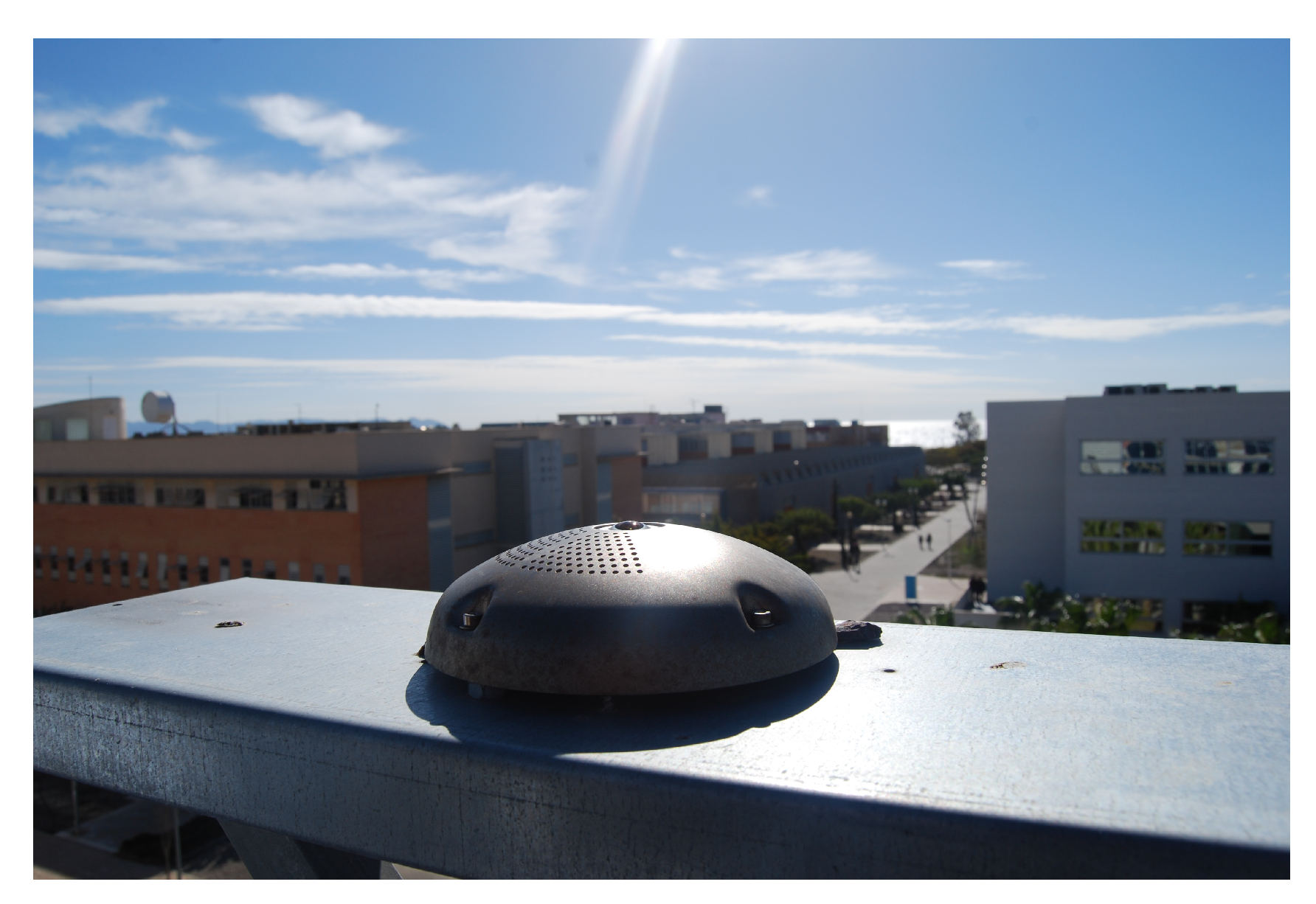
This work used images from a hemispheric low-cost sky camera, (model Mobotix Q24), placed on the rooftop of the Solar Energy Research Center (CIESOL) at the University of Almería, Spain (36.8°N, 2.4°W; at sea level). Figure 1 shows the camera installation on the CIESOL building.

The facility’s location has a Mediterranean climate with a high maritime aerosol presence. The images produced are high resolution from a fully digital color CMOS (2048 × 1536 pixels). One image is recorded every minute in JPEG format, the optimal time for identifying clouds in the sky. The three distinct channels represent the red, green and blue levels. Each image pixel is made up of 8 bits, resulting in values of between 0 and 255.

For this work, images were selected from all possible sky types, spanning the earliest times of the day to just before sunset, and at different times of the year. The period studied was from 2013 to 2019.

For this work, images were selected from all possible sky types, spanning the earliest times of the day to the latest, just before sunset, and at different times of the year. The period studied was from 2013 to 2019.

3. Methodology

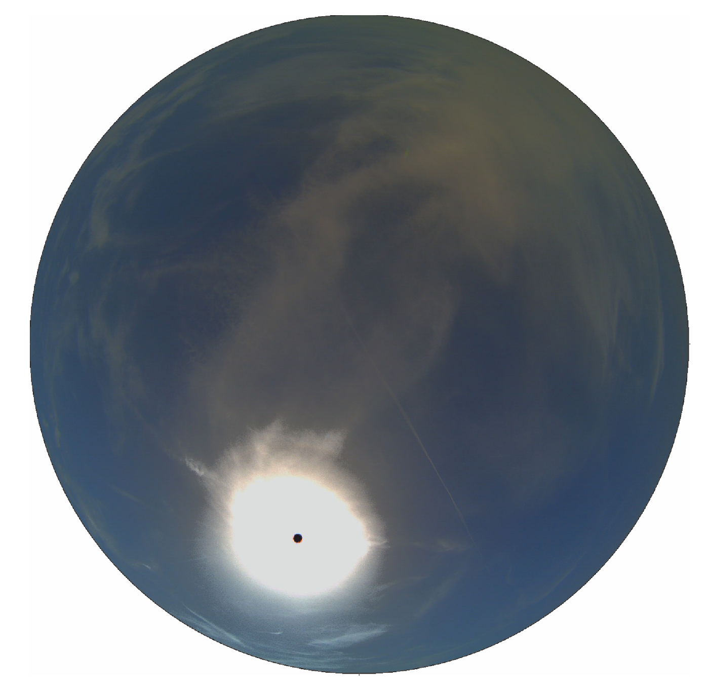
This section describes the particular tasks undertaken to find the different clouds that can appear in a sky capture, defining the methodology and the steps involved to process an image. All developments have been carried out in the MATLAB environment as it is the optimal platform for operating with matrices in record time. Its efficiency is the main reason this software was used for the methodology. As the starting point, a raw image is presented in Figure 2, where the sky is represented as a common image.

Here, we see the circular representation of the sky appearing over a black background. The first step is to determine the area of interest from the raw image by applying a white mask, thus obtaining the image seen in Figure 3, where the sky is perfectly identified in the circular area.

After applying this customized mask, the image is ready for use in the developed algorithm to detect clouds. The MATLAB environment allows one to make changes in the image’s color space so that specific properties can be studied. This is the case with HSV (Hue, Saturation, Value), NTSC and yCbCr color spaces. The first, HSV, gives information about the gray color scale, where pixels vary between 0 and 1. The second, NTSC, is really an RGB color space, where the first component, luminance, represents grayscale information and the latter two components make up the chrominance (color information). The last, yCbCr, is used to digitally encode the color information in the computing systems: y represents the brightness of the color, Cb is the blue component relative to the green component and Cr is the red component relative to the green component. Figure 4 shows the image presented beforehand in the three color spaces.

The different colors of the three images represent the main image characteristics. Focusing solely on the inside of the circle, the blue color identifies the more saturated areas of the HSV image. These areas are represented by red and yellow in the NTSC image, and by orange, rose and red in the yCbCr image. Normally, in the NTSC and yCbCr color spaces, the pixel values acquire inflexible static values in each color space channel whereas in the HSV color space, the pixels (represented by the three bands/channels) provide values with better precision for the purpose of cloud detection. Moreover, the clouds are not perfectly represented in the three color spaces so it is important to define the most significant color space to work with. Given that the HSV color space represents cloudy pixels better (including those clouds that are more difficult to classify), and more clearly, it has been used together with the RGB color space to identify clouds in the image processing procedure [13,14,20]. For the complete image processing procedure, the developed algorithm was structured into different parts, as described in the following subsections. The different tables define specific criteria for image processing. Basically, each table has been created for the purpose of each subsection and to set the intensity levels of the channels, so as to precisely detect the zones (clouds or sky). To obtain a special classification of the pixels in each zone, different labels are defined and attributed to the pixels, as shown in

Table 1. Criteria for labeling pixels in the whole sky cam image.

Pixel Label	Color Assigned	Pixel Condition
256	Green	Initial saturated pixels
257	White	Cloudy pixel in the solar area
258	White	Cloudy pixel in general (excluding solar area)
259	Blue	Cloudless pixel in general (excluding solar area)
260	Red	Cloudless pixel in the solar area
261	Yellow	Pixels around solar area with intermediate bright

.

To accomplish this, different images have been analyzed at different times of the day and at different times of the year. Following this, a general initial state has been assumed to precisely adjust the intensity values. Normally, the general state of each table starts by analyzing the R value and the comparison with the G and B channels. If the intensities of these channels are enclosed in particular values, the HSV channels are also analyzed. The uncertainty of each channel is the sensitivity of each one, i.e., in the RGB color space, ±1, it is ±0.001 for the H channel, ±0.0001 for the S channel and ±1 for the V channel. Therefore, this algorithm has been gradually formed in parts so that in the end, it remains connected and sequential, in the same order as it appears in the manuscript.

3.1. Recognition of the Solar Area: Classification of Pixels

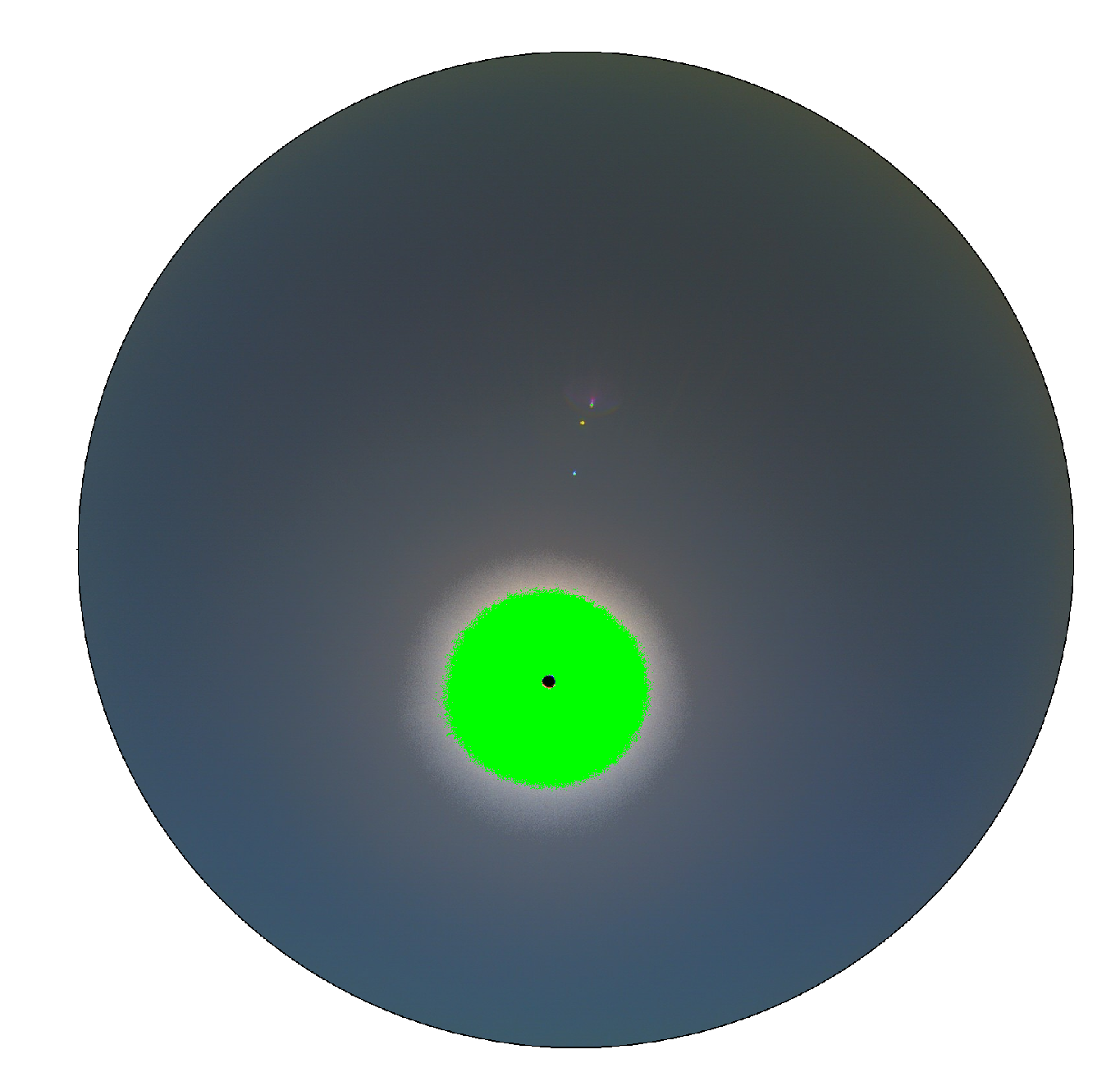
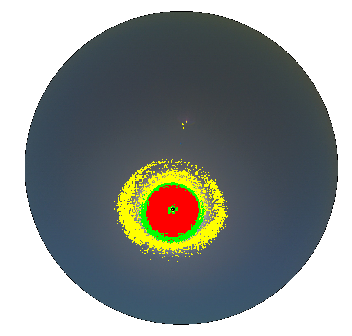
The first step for detecting clouds in the whole sky image is to determine the solar area. Being able to recognize this area is fundamental for establishing the sun’s position in the image. To track the angle of solar altitude $\left(\alpha \right)$ at each minute, the Cartesian coordinates are obtained, with the south represented by the bottom-center pixels and the east by the centeR − right pixels. Subsequently, the original image (in JPG format), defined by the RGB color space, is also converted into the HSV color space. As seen in the previous images, the sun appears as bright pixels, so one needs to consider the position of the pixels to determine the bright solar pixels. To do this, after locating the sun pixel (according to the solar altitude and azimuthal angles), a matrix is created to determine the distance of the other pixels from it (Dis). This operation allows one to classify whether a bright pixel is a ‘solar pixel’ or not (based on its position). As a general rule, when the value of the red, blue and green pixels is greater than 160, the pixels are identified as being in the sun area. Figure 5 shows the general detection of the sun pixels.

The main step consists of applying a green mask to pixels that are placed in the sun area. After that, the idea is to detect if these pixels are cloudless or overcast.

Table 2. Criteria for selecting cloudless pixels in the solar area.

Red (R)	Green (G)	Blue (B)	Hue (H)	Saturation (S)	Special Condition
[171,180]	-	-	0	0	R = G & G = B
[225,235]	-	R − 2	(0.166, 0.168)	(0.0070, 0.0100)	R = G
≥200	-	R − 2	(0.166, 0.168)	(0.0070, 0.0100)	R = G
228	-	R − 2	(0.166, 0.168)	(0.008, 0.009)	R = G
≥230	-	-	>0	-	R = G & G = B
≥210	-	-	≥0.416	≤0.005	-
[173,218]	-	-	[0.416, 0.418]	(0.0112, 0.1130)	Dis < 135
[173,178]	≥178	-	(0.166, 0.168)	(0.0110, 0.1120)	Dis ≥ 135
[172,177]	-	-	(0.166, 0.168)	(0.0100, 0.1113]	R = G
≥176	-	R − 2	≠0.167	-	Dis < 135 & R = G
≥176	-	R − 2	(0.166, 0.168)	(0.0103, 0.0107)	Dis < 135 & R = G
≥172	-	-	(0.416, 0.418)	(0.0109, 0.0113)	R = (G − 2) & R = (B − 1)
≥180	-	-	(0.166, 0.168)	(0.0100, 0.0110)	R = G & R = (B + 2)
≥172	-	-	(0.416, 0.418)	(0.0105, 0.0107)	R = (G − 2) & R = (B − 1)
[172,185]	-	-	(0.166, 0.168)	(0.0112, 0.0113)	R = G & R = (B + 2)
[170,174]	R + 2	R + 1	(0.416, 0.418)	(0.0107, 0.0109)	-
[190,194]	R + 2	R + 1	(0.166, 0.168)	(0.0112, 0.0113)	R = G & R = (B + 2)
194	R + 2	R − 1	(0.277, 0.279)	(0.0152, 0.154)	-
≥225	≥225	≥225	0	0	$\alpha$ ≤ 14
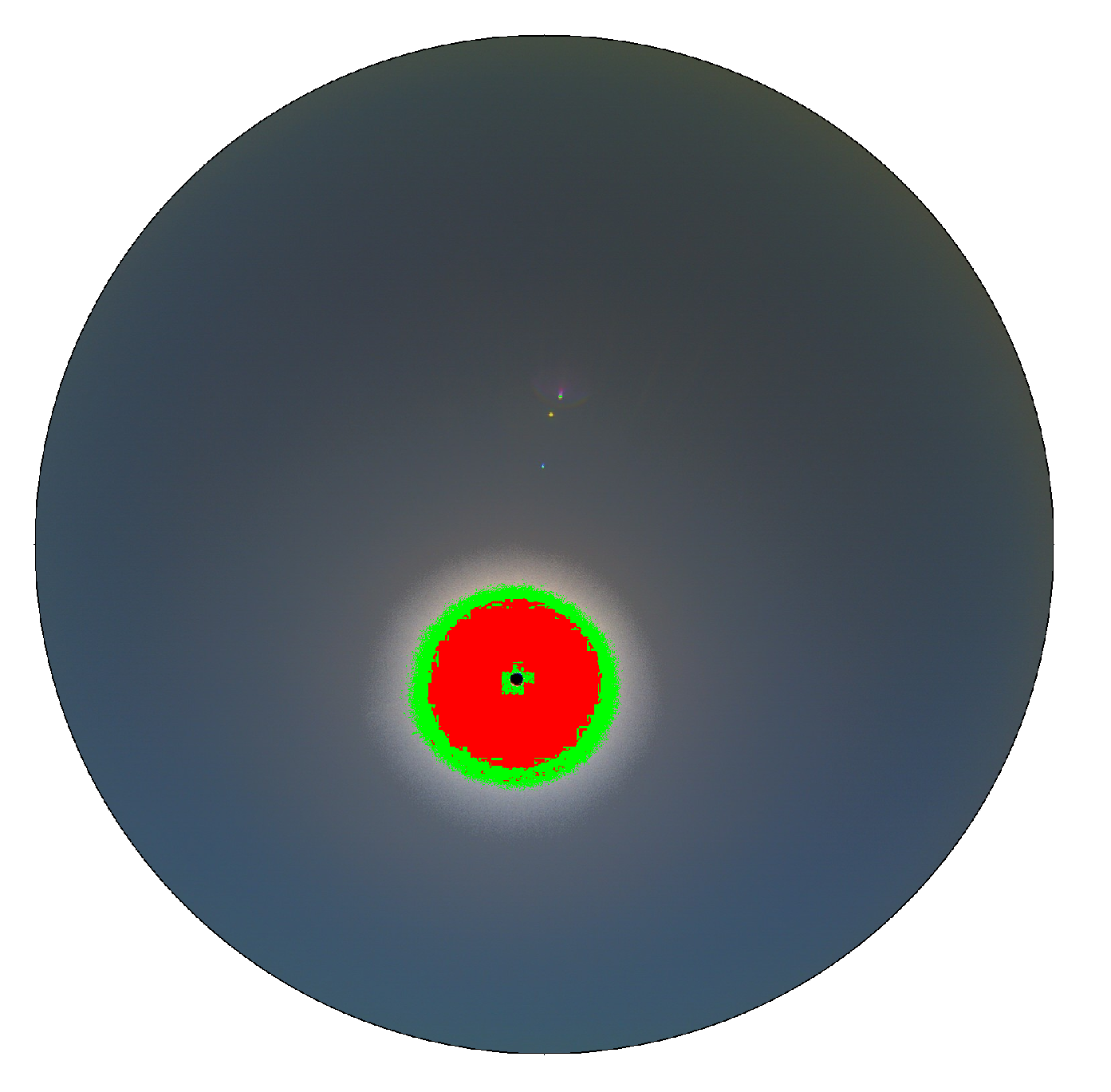
≥200	≥200	≥200	[0.416, 0.418]	≥0.0080	$\alpha$ ≤ 14

shows the rules for determining cloudless pixels in the solar area. In general, the table collects the relationships between the pixel levels (according to the corresponding channel) that satisfy the criteria for determining cloudless pixels in the solar area. The parameters and thresholds have been defined based on the cases studied for the proposed model.

After the different strategies have been carried out to determine the cloudless pixels in the sun area, according to the pixel intensity in each image channel (Table 2), Figure 6 shows the general detection of the cloudless pixels in the sun area (represented in red) after this filter has been applied.

Subsequently, the algorithm looks for cloudy pixels in the same area to detect if any clouds are present.

Table 3. Criteria for selecting cloudy pixels in the solar area.

Red (R)	Green (G)	Blue (B)	Hue (H)	Saturation (S)	Special Condition
≥172	-	-	<0.168	≥0.013	R = G

shows the condition for classifying the pixels in the solar area as cloudy.

Only one sentence (criterion) is applied for detecting cloudy pixels in the solar area. In these situations, when a cloud is identified by means of a pixel, the mask applied is also green. When the solar area has been fully treated, the algorithm focuses on the rest of the image, starting with the solar area periphery.

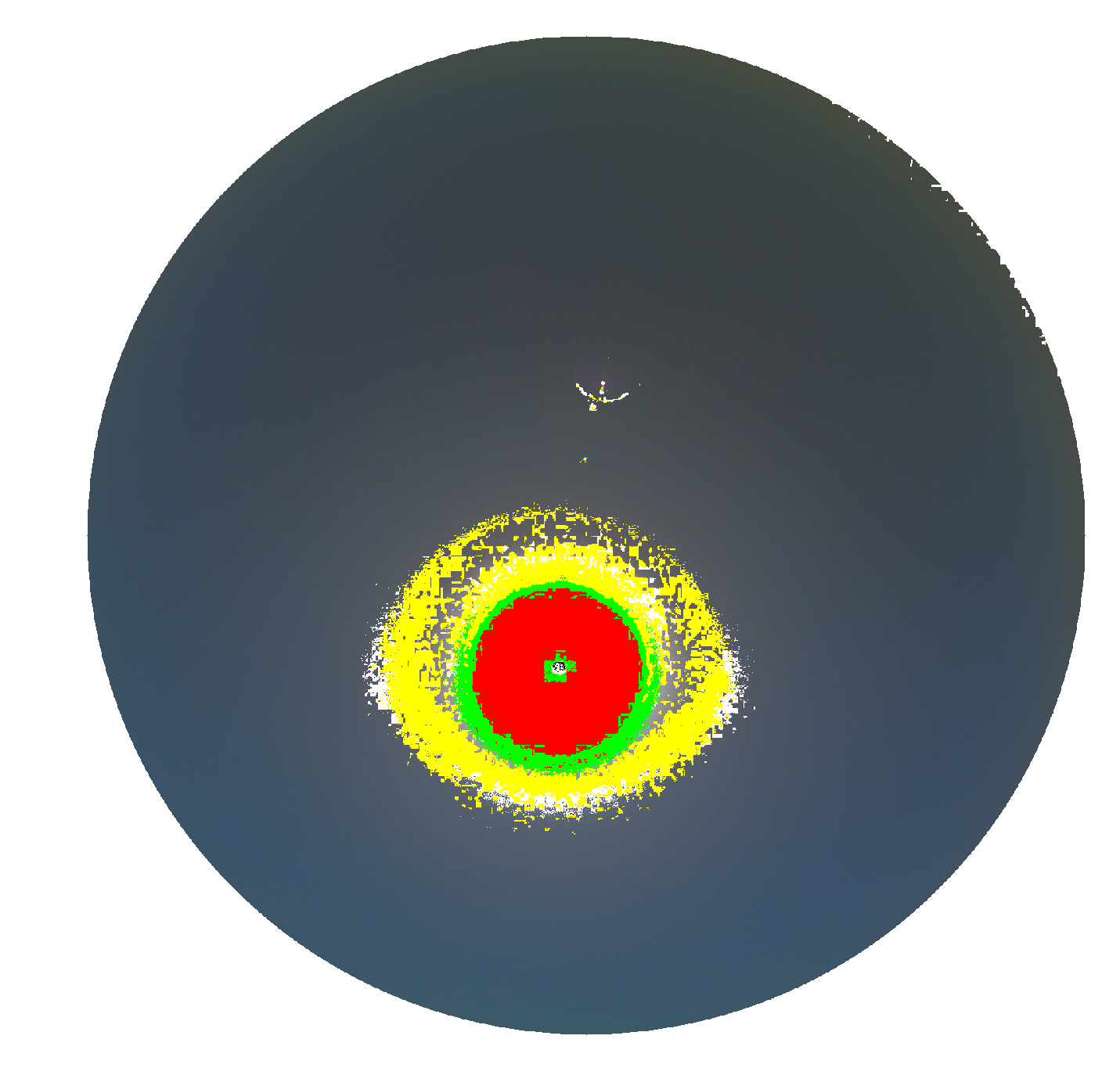
3.2. Detection of Bright Zones around the Solar Area

The pixels located around the solar area have an intermediate bright characteristic. In other words, the pixels present values lower than the solar area pixels but higher than those in the rest of the image. The size of this area varies according to the day and the atmospheric conditions at each moment.

Table 4. Criteria for detecting bright pixels around the solar area.

Red (R)	Green (G)	Blue (B)	Hue (H)	Saturation (S)	Special Condition
>125	-	-	-	-	(B − R > 8) & (B − 4 > 4)
130	≥140	≥150	-	≥0.1900	Dis < 650
(130,140)	≥150	≥159	-	≥0.1900	Dis < 650
[140,150)	≥160	≥169	-	≥0.1900	Dis < 650
[150,165]	≥165	≥175	-	≥0.1900	Dis < 650
>130	-	-	-	-	(Dis < 650) & (B − R > 30)
>130	≠R	-	<0.1	≥0.1000	(Dis < 650) & (R − G ≥ 8)
-	>110	-	-	-	(Dis < 650) & (G > R) & (G > B) & (G − R < 8)
>140	-	-	-	-	(Dis < 650) & (R − G ≤ 10) & (R − B ≥ 25)
(≠ 257) & (≠ 260)	≥130	-	[0.400, 0.580]	≤0.0800	(Dis < 650)
(≠ 257) & (≠ 260)	-	-	≤0.090	≤0.0900	(Dis < 650)
(≠ 257) & (≠ 260)	-	-	≤0.090	≤0.0900	(Dis < 650) & (G < R) & (R − G < 8) & (∣G − B∣ < 3)
(≥100) & (≠ 257) & (≠ 260)	-	-	-	-	(Dis < 650) & (G − R > 20) & (B − R > 35)
(≥100) & (≠ 257) & (≠ 260)	-	-	-	-	(Dis < 650) & (G − R > 20) & (B − R > 35)

shows the adjusted criteria for determining these pixels.

One of the most important tasks is to locate each pixel. The $Dis$ variable almost always appears because the pixel emplacement is very important in this process. Therefore, to distinguish previously classified areas in subsequent processes, the yellow color is used to mark the new area (Figure 7).

The new pixels classified as yellow do not represent a homogeneous area; they are dispersed across the image but at a distance of less than 650 units from the central solar pixel. In this new preprocessing, there are gaps between the yellow and green pixels that need to be classified beforehand. With the solar and surrounding area processed, the algorithm looks for cloudy pixels in the rest of the image.

3.3. Detection of Cloudy Pixels in the Rest of the Image

In general, clouds present several characteristics that allow us to identify the most common cloud types (white or extremely dark clouds).

Table 5. Criteria for cloud detection excluding the solar area.

Red (R)	Green (G)	Blue (B)	Hue (H)	Saturation (S)	Special Condition
B	B	-	-	-	-
≠[259,261]	-	-	-	>0.2500	(V ≠ 256) & (R ≥ B)
≠[259,261]	-	≥100	-	≤0.1800	(V ≠ 256) & (R/B ≤ 0.90)
≠[259,261]	-	-	≤0.200	≤0.2000	(V ≠ 256)
≠45	-	≥80	<0.600	≥0.3500	-

shows the general pattern for detecting the clouds in the complete image by characterizing the digital levels of these common cloud types.

If a cloudy pixel is detected, it is marked in white. There are many cases in which some pixels are identified as cloudy although no clouds are present in the sky. This is caused by the similarity in the range of channel values, whereby dark skies can be confused for dark clouds. However, this mistake can be remedied during the algorithm’s following steps. An example is presented in Figure 8, where certain pixels are classified as cloudy in color white.

Only a few pixels are classified as cloudy near the sun area. The first picture for this day showed no clouds appearing in the image, thus no cloudy pixels could be generated. Despite this, a few pixels are interpreted as cloud. When solar area pixels and cloudy pixels are evaluated, the process continues to detect the pixels as unclassified.

3.4. Detection of Cloudless Pixels in the Image Excluding the Solar Area

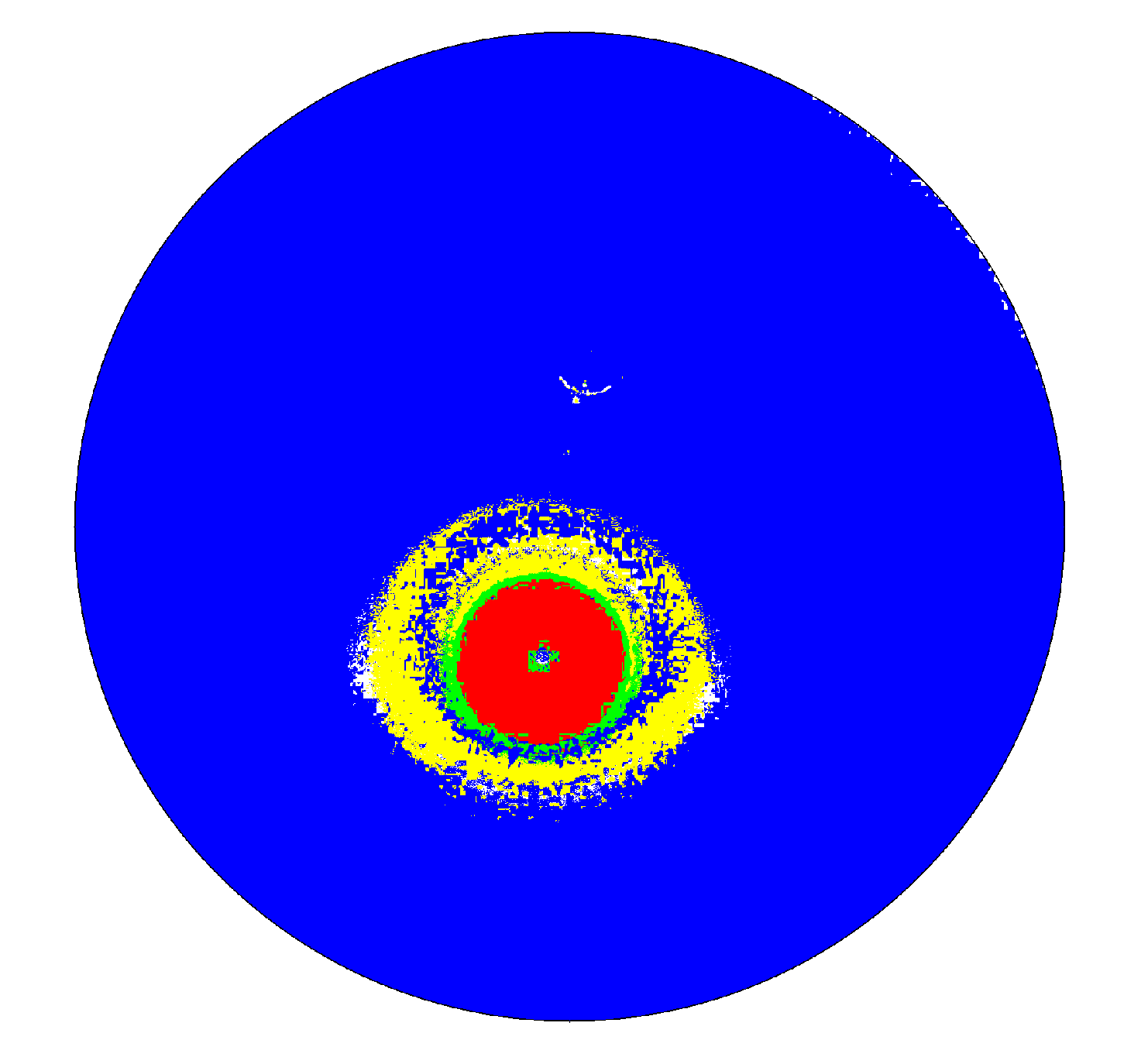
After the solar area has been classified, the rest of the image is analyzed to identify if a pixel represents a cloud or not.

Table 6. Criteria for detecting cloudless pixels in the image excepting in the solar area.

Red (R)	Green (G)	Blue (B)	Hue (H)	Saturation (S)	Special Condition
-	-	≤83	≥0.250	≥0.3000	-
≥55	-	≤83	≥0.580	≥0.5700	-
≤52	-	≥100	≥0.570	≥0.5700	-
≤50	≤60	≥83	≥0.610	-	-
-	-	-	≥0.500	≥0.4500	-
[50,60]	[57,63]	[66,75]	[0.610, 0.650]	[0.2000, 0.3000]	-
≤70	-	≥75	≤0.700	≤0.3100	-
≥55	-	-	≥0.600	-	R/B ≤ 0.80
[50,68]	-	-	-	≥0.4600	R/B ≤ 0.80
>G	-	-	≥0.660	-	(R/B ≥ 0.94) & (G/B ≥ 0.88)
-	-	≥90	≥0.620	-	-
-	-	≥115	≥0.550	≥0.3000	-
-	-	-	≥0.800	-	-
[65,72]	[80,90]	≥108	-	-	-
[49,54]	[60,69]	[86,93]	-	-	-
G	-	-	-	-	B > G
≥100	≥110	≥130	-	-	-
-	B	>70	-	-	R < B
[70,75]	-	[84,89]	-	-	G − R < 4
-	-	[90,100]	-	-	(G − R $\mathsf{ϵ}$ [6,7]) & (G − R $\mathsf{ϵ}$ [9,12]))
-	-	-	-	-	(|R − B| ≤ 3) & (G>B) & (R/G $\mathsf{ϵ}$ [0.90, 0.92])
[80,85]	[82,90]	[88,94]	-	-	(G − R ≤ 3) & (B − R ≤ 7)
[59,64]	[69,75]	-	-	-	(G − R ≥ 6) & (B − R ≥ 12)

represents the set of sentences implemented to detect the cloud-free pixels in the parts of the image that do not include the solar area.

One can see that the $Dis$ variable was not used even though we have presented the criteria to identify the pixels outside the solar area have been presented. This is because, for cloudy pixels, the digital pixel levels never appear in the range levels shown in the table. For this reason, it was not necessary to include the aforementioned variable in the sentences used (Figure 9).

In the image, the sun area and the surrounding area are processed, along with a small part of the remaining image. Therefore, at this point in the algorithm, it is still possible that a large part of the image has not been processed. Consequently, a further step is needed to conclude the algorithm and classify all the pixels.

3.5. Determination of Non-Classified Pixels

The final steps for classifying the pixels in a complete image establish a statistical criterion based on the pixels that have already been classified. Knowing the number of pixels for each color, we determine those pixels that do not have a label. There are different strategies for establishing the classification criteria of these, as yet unclassified pixels.

Table 7. Criteria for the determination of cloudless pixels for non-labeled pixels.

Main Condition	Other Conditions
$\alpha$ < 5	(SkyPixels > 1,000,000) & (RedPixels ≥ 7000)
$\alpha$ ≥ 5	CloudPixels ≤ 25,000
$\alpha$ ≥ 5	(CloudPixels > 25,000) & (GreenPixels ≤ 1.6 RedPixels)
$\alpha$ ≥ 5	(CloudPixels > 25,000) & (RedPixels ≥ 0.7 (GreenPixels + YellowPixles))
$\alpha$ ≥ 5	(CloudPixels > 25,000) & (NonClass ≥ 1,100,000 & (RedPixels ≥ 2 GreenPixels) & (SkyPixels > CloudPixels))
$\alpha$ ≥ 5	(CloudPixels > 25,000) & (NonClass ≥ 800,000 & (SkyPixels ≥ 400,000) & (CloudPixels ≤ 140,000))
$\alpha$ ≥ 5	(CloudPixels > 25,000) & (NonClass ≥ 600,000 & (SkyPixels ≥ 700,000) & (CloudPixels ≤ 120,000))

shows the steps to determine whether the pixels should be classified as cloudless; if not, they will be classified as cloudy.

In the table, different expressions appear. $SkyPixels$ are pixels that have been classified as cloudless, whereas $CloudPixels$ are those that have been labeled as cloudy. Red, green and yellow pixels have been obtained in the previous processes and $NonClass$ is used to refer to the pixels that remain unclassified. For these operations, the MATLAB environment allows one to perform matrix operations in an efficient way. This part of the algorithm results in a matrix where all the pixels have been labeled, as shown in Figure 10.

As one can see, all the pixels have been assigned a color: blue, yellow, red or green. Now, the aim is to finish the classification process according to a common criterion.

3.6. Final Step in the Sky Cam Image Classification

To finish the sky cam image processing, a final step is needed in which the differently colored pixels are converted so one can determine whether they are cloudless or cloudy. This process has been developed from experience gathered working with a great number of images and scenarios.

Table 8. Criteria for the last classification of pixels in the sky cam image processing.

Label	Classification Conditions	Final Classification
Green	(Dis ≥ 700)	Cloud
Yellow	(Dis ≥ 700)	Cloud
Green/Yellow	($\alpha$ ≥ 5) & (RedPixels ≥ 0.5 GreenPixels) & (GreenPixels > 25,000)	Cloudless
Green/Yellow	($\alpha$ ≥ 5) & (RedPixels ≥ 0.3 GreenPixels) & (SkyPixels ≥ 1,000,000)	Cloudless
Green/Yellow	($\alpha$ ≥ 5) & (RedPixels ≥ 0.3 GreenPixels) & (RedPixels ≤ 15,000)	Cloud
Green/Yellow	($\alpha$ ≥ 5) & (RedPixels ≥ 0.3 GreenPixels) & (CloudPixels ≥ 500,000) & (RedPixels ≤ 0.5 GreenPixels)	Cloud
Green/Yellow	($\alpha$ ≥ 5) & (RedPixels ≥ 0.3 GreenPixels) & (CloudPixels ≥ 500,000) & (GreenPixels ≤ 25,000)	Cloud
Green/Yellow	($\alpha$ ≥ 5) & (RedPixels ≥ 0.3 GreenPixels) & (CloudPixels ≥ 500,000) & (RedPixels $ϵ$ [15,000,30,000])	Cloud
Green/Yellow	($\alpha$ ≥ 5) & (RedPixels ≥ 0.5 GreenPixels) & (GreenPixels > 25,000)	Cloudless
Green/Yellow	($\alpha$ ≥ 5) & (RedPixels ≥ 0.3 GreenPixels) & (SkyPixels ≥ 1,000,000)	Cloudless
Green/Yellow	($\alpha$ ≥ 5) & (SkyPixels ≥ 1,000,000) & (RedPixels ≤ 15,000)	Cloud
Green/Yellow	($\alpha$ ≥ 5) & (SkyPixels ≥ 1,000,000) & (CloudPixels ≥ 500,000) & (RedPixels ≤ 0.5 GreenPixels)	Cloud
Green/Yellow	($\alpha$ ≥ 5) & (SkyPixels ≥ 1,000,000) & (CloudPixels ≥ 500,000) & (GreenPixels ≤ 25,000)	Cloud
Green/Yellow	($\alpha$ ≥ 5) & (SkyPixels ≥ 1,000,000) & (CloudPixels ≥ 500,000) & (RedPixels $ϵ$ [15,000,30,000])	Cloud
Green/Yellow	($\alpha$ < 5) & (RedPixels ≥ 7000)	Cloudless
Green/Yellow	($\alpha$ < 5) & (RedPixels ≥ 3 GreenPixels)	Cloudless
Green/Yellow	($\alpha$ < 5) & (RedPixels ≥ 10,000) & (SkyPixels ≥ 1,000,000)	Cloudless
Green/Yellow	OtheR − case	Cloud
Red	(Dis ≥ 700)	Cloud
Red	-	Cloudless

shows the specific criterion for assigning the final pixel classification.

Following the assignations in the table, the final image can be generated, the result of which is shown in Figure 11.

The criteria presented in the above tables have been carefully defined, thus changes in the correlations represent alterations in the final processed image. Each criterion has an associated sensitivity according to the number of pixels involved (the pixels that fulfill the determined criteria). Therefore, the sensitivity associated with each criterion affects the pixels that fulfill the condition and, consequently, the final processed image. An error in one of the criteria presented in the tables would mean a cloud detection error, and therefore the image would not have been processed in a valid way and would be identified as wrong.

4. Results

In this section, we present the results of the cloud detection algorithm. To analyze the behavior of the software developed under different sky conditions, this section presents several pictures from various sky scenarios. A total of 850 images were taken from 2013 to 2019 at different times (from sunrise to sunset). The images were processed with the analytical objective of obtaining an accurate identification of clear sky and clouds. Therefore, this section is divided into subsections.

4.1. Sky Images Processed under all Sky Conditions

To analyze the quality of the developed model, several images have been processed and studied. In general, the processed image should show the most important clouds appearing in the original image (when visually inspected). The important clouds are those that can be identified clearly (not only by a few pixels). To view several examples, the following figures represent the image processing procedures carried out for the algorithm that was presented in the previous section. 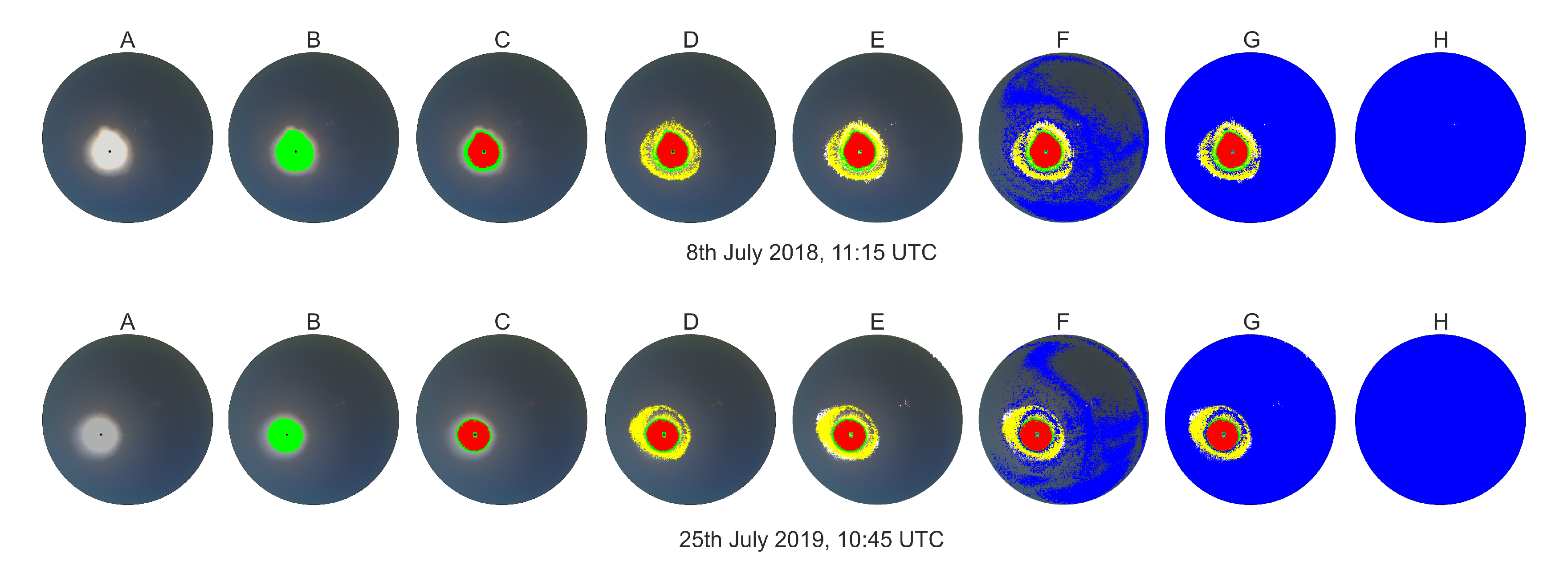Figure 12 shows two examples chosen randomly, in which a clear and cloudless sky appear.

In the case of cloudless skies, the sun can vary its form and size depending on the solar altitude angle. The algorithm contemplates this angle to identify clouds based on the variability in pixel intensity according to the sun position. Specifically, the sun is the key intensity point of the pixel value and the solar position determines a pathway for performing the cloud recognition. Despite this, for the two cloudless days represented in the image, the sky is free of clouds, as represented by images with the letter H. As one can observe, for each original image (marked with the letter A), a sequence of images appears showing the steps the algorithm takes to finally obtain the image (by identifying the sky and cloudy pixels). In these cases, no cloud was detected and, therefore, the final images are completely blue.

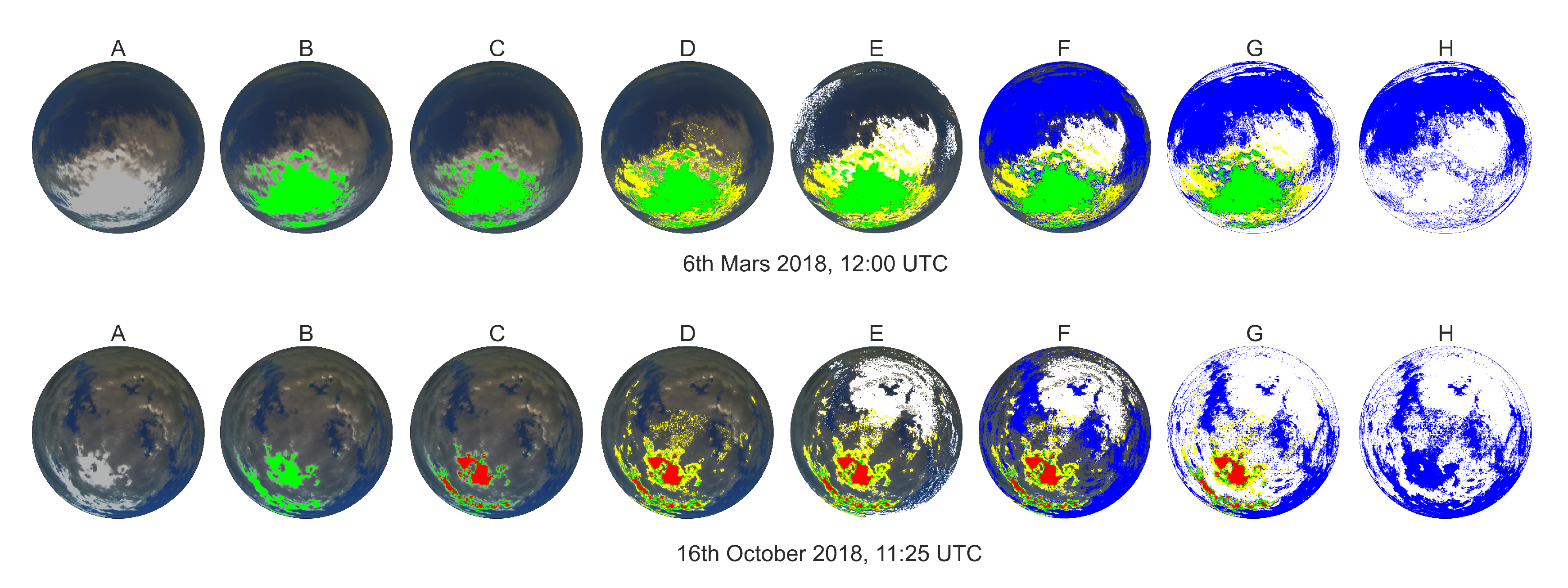
When the sky is not completely free of clouds, it can be either partially or completely covered. In the first case, varying portions of the sky and cloud may appear when observing a sky camera image. Therefore, it is important to determine the boundaries between the cloud and the sky as effectively as possible. Figure 13 shows two different partially cloudy situations.

Two scenes have been represented for cloud identification, each differing in various ways. In the first sequence of images (the top line), one can appreciate how most of the clouds are around the solar area. In images B and C, the algorithm recognizes the large green and yellow areas. Subsequently, clouds are detected in the adjoining areas (image E) before finally classifying those green and yellow pixels as a cloud. In the other image sequence (the bottom line), the area detected in green turns red where the sun appears. This is because the algorithm’s established criteria have not been met for identifying the pixels as a cloud; therefore, they are marked in red. Following this, the clouds are optimally detected in image E and the blue sky is detected in image F. Finally, the image is resolved, classifying the pixels in red, green and yellow as cloudless. It is curious how the clouds have generated significant brightness in the solar area, mistakenly classifying the solar area pixels as clouds.

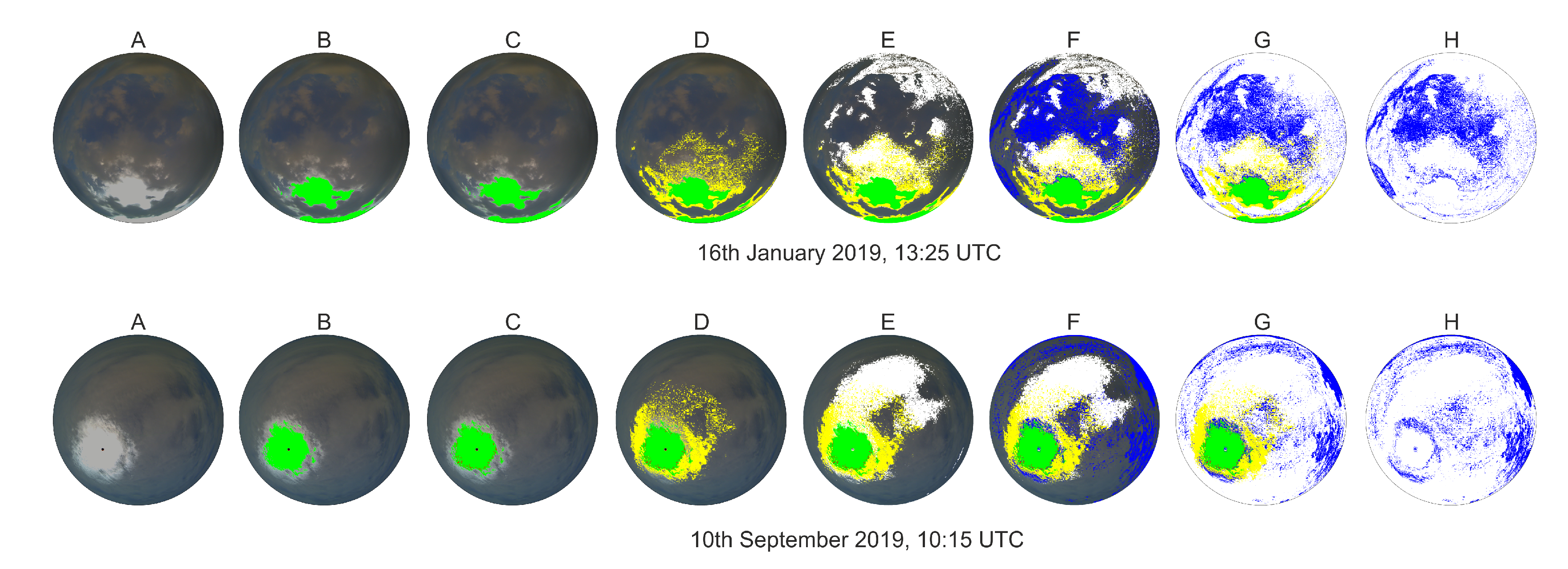
Figure 14 shows two cases in which virtually the entire image is covered by clouds.

The top sequence of images shows a day when there was a lot of cloudiness and only small portions of sky. As the algorithm is executed, it is interesting to see how no red zone is detected (attributing the solar area as cloudless) because the clouds in this case have a profile that is perfectly identified by the set of sentences presented in the previous tables. Here, the breaking clouds have been correctly classified in image F. To conclude, image H shows the result of the process with the identification and classification of all the processed pixels being virtually identical to the original image. The bottom image sequence shows another day when there were more clouds in the image, and again one can observe that no red pixels have appeared. By following the steps described in the previous sections, the image processing very precisely determines the areas of blue sky and clouds (image H).

4.2. Statistical Results and Comparison with TSI-880

To make a statistical evaluation of the developed model’s efficacy, we used a model that is already established and published [13,21]. This model works with images from a sky camera (installed on the CIESOL building) that has a rotational shadow band (the TSI-880 model) providing a hemispheric view of the sky (fish-eye vision). In short, the TSI-880 camera model is based on a sky classification that uses direct, diffuse and global radiation data. The sky is classified as clear, covered or partially covered. For each sky type, digital image processing is performed, and an image is obtained with the cloud identification. 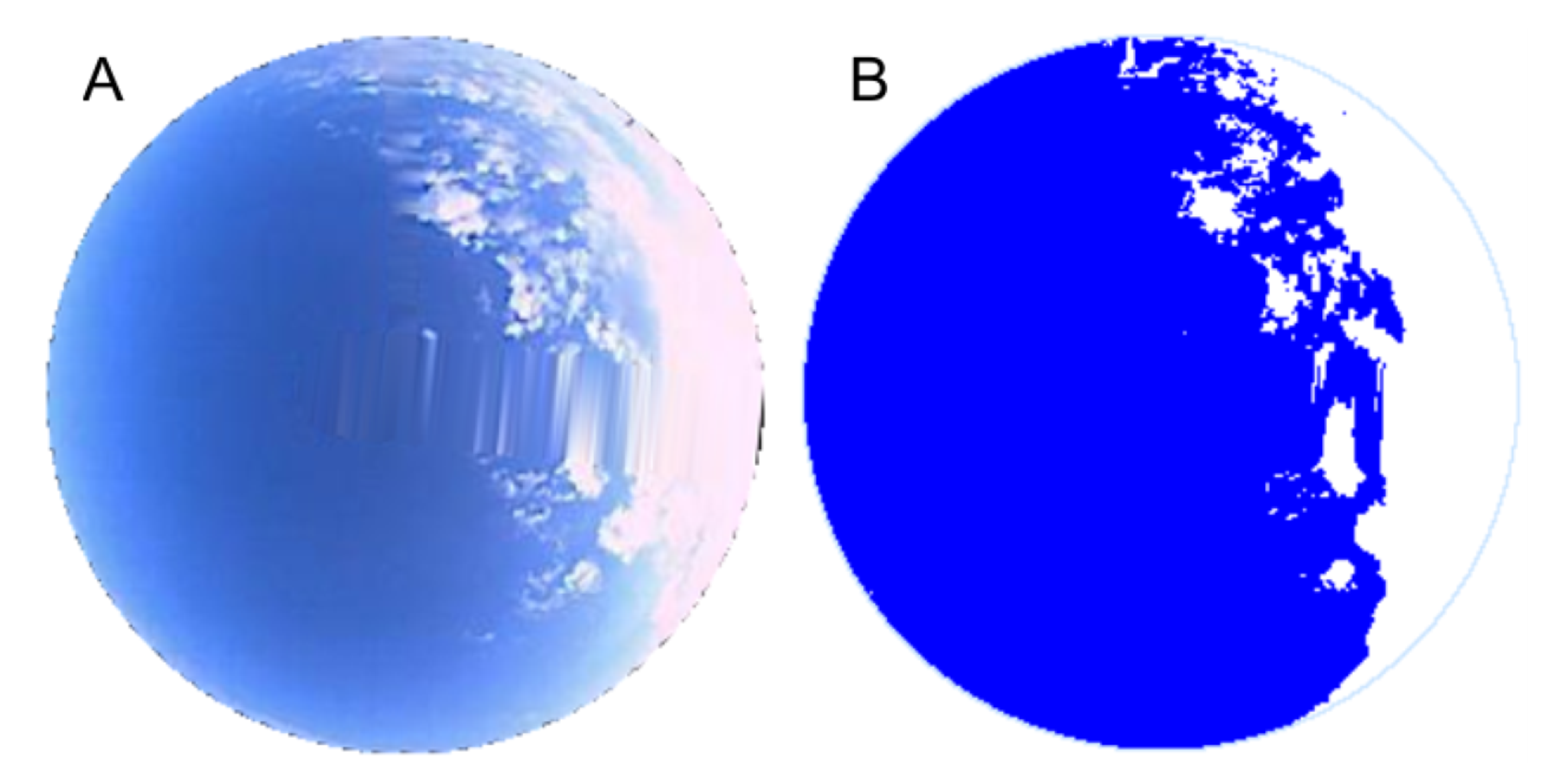Figure 15 shows an example of a partially cloudy day at a time shortly after sunrise.

Looking at the TSI-880 camera image, it is significant how the pixel intensities are very different from those represented by the Mobotix camera. The blue sky generally appears lighter because of the camera’s optics. For this reason, it is not possible to extrapolate the development of the TSI-880 camera to that of the Mobotix Q24 camera.

Taking this model as a reference, a total of 845 images were taken between the months of August and December 2013 (by that time, the images from both cameras were available). To make the comparison, a routine was established whereby an image was taken approximately once an hour (whenever possible) and the images from both cameras were processed. In total, 419 images corresponded to clear skies, 202 to partially covered skies and 224 to overcast skies. A probability function was used to determine the model’s success rate in percentage values. It was considered a success if the processed image represented the original image; that is to say, it differentiated the areas of clear sky and clouds correctly. Equation (1) shows the probability function ($PF$):

$$PF(\%)=100·\frac{Successes}{Totalcases},$$

(1)

In Equation (1), two variables are defined: Successes and Total cases. The first is based on obtaining a processed image with practically perfect cloud identification. Almost perfect means that the processed image adequately represents what appears in the original image (either with the TSI-880 camera or with the Mobotix camera). Therefore, a hit will be a final processed image that is like the original. The total number of cases will be the total number of images analyzed. The evaluation is done visually since there is no tool capable of detecting the difference between a raw and a processed image (that is why a cloud detection algorithm is so valuable). In this sense, the reference is always the original image, and any processed image should resemble the original.

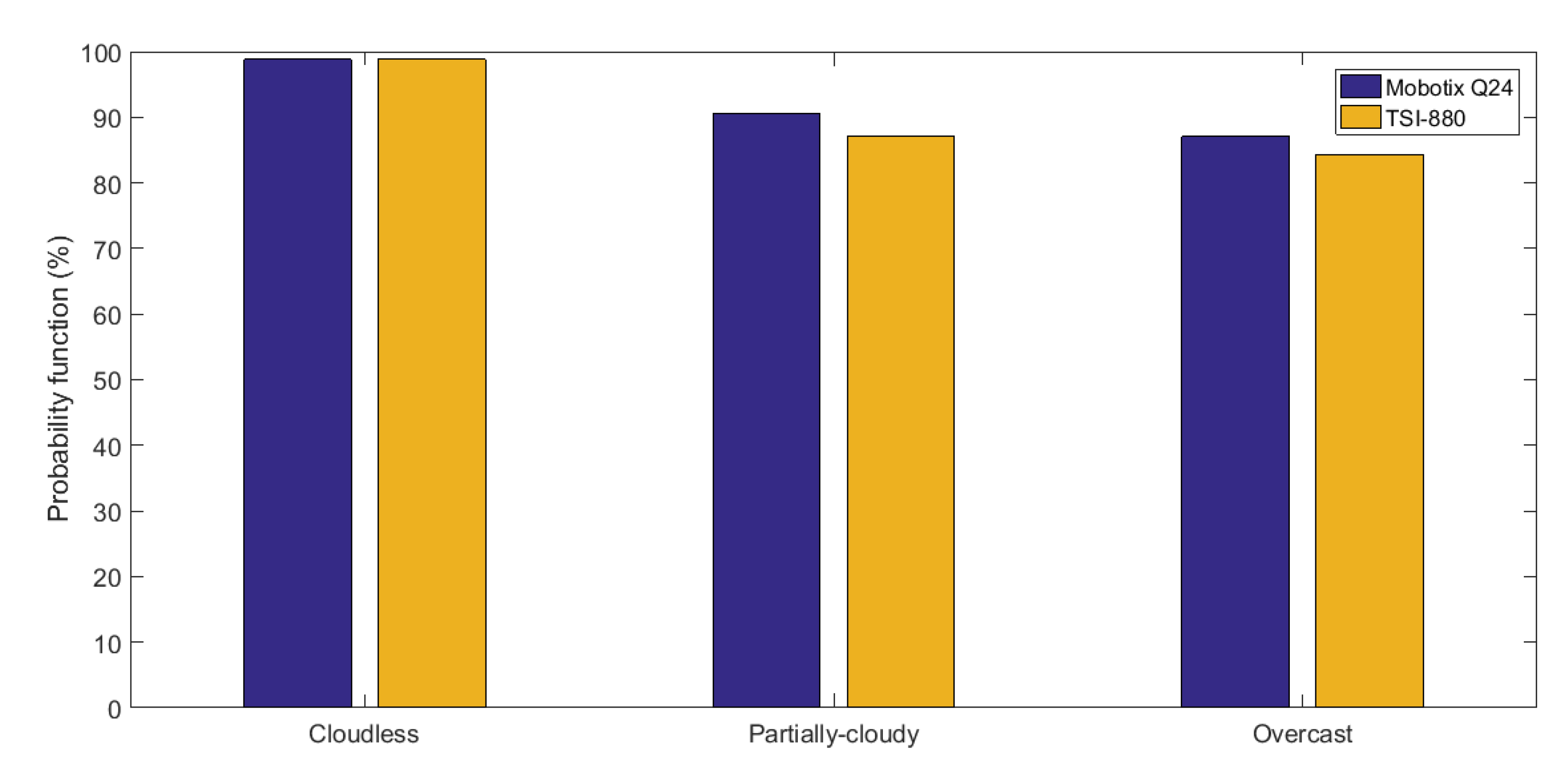
Figure 16 shows the image processing efficacy once the function was defined by comparing the Mobotix Q24 camera to the TSI-880 camera in terms of the sky classification.

The results have been divided into three basic groups: one representing the probabilistic results for clear skies, another for partially covered skies and the third for covered skies. In each group, a bar represents the success rate in (%). As one can observe, all the presented results are above 80%. The best results were obtained for clear skies, where the two cameras had the same success rate, 98.8%. For partially covered skies, the Q24 camera provided better results than the TSI-880, with a success rate of 90.6% (the TSI-880 success rate was 87.1%). In the case of overcast skies, the Mobotix camera again had a higher success rate, at 87.1%, while the TSI-880 camera had a value of 84.4%. In general, one can say that the cameras had a very similar success rate despite the slight differences found on days with clouds. Figure 17 shows a comparative graph of the overall hits in cloud detection.

As can be seen in the graph, the two cameras had very similar values overall; the cloud detection image processing for the Mobotix camera had a success rate of 93.7% while the TSI-880 camera had a value of 92.3%.

In addition, it should be noted that the TSI-880 camera requires a high level of maintenance to ensure the optimal quality of the images taken; this is due to its special design, in which the glass is a rotating dome that must be cleaned periodically, taking care not to scratch it. Moreover, the glass is rotated by a motor that needs to be checked regularly to ensure proper operation. In contrast, the MobotixQ24 camera is similar in dimension to a surveillance camera, with only a small glass panel protecting the lens; this means that its maintenance requirements are significantly less. For this work, one can state that it was not necessary to clean the glass for several months. The device produced sharp, appropriate images allowing the algorithm to correctly identify the clouds present. Consequently, this article demonstrates that a new algorithm has been developed which is capable of offering the same performance as the TSI-880 camera, without the need for radiation measurements to perform the digital image processing and requiring only minimal maintenance to acquire quality images for the cloud detection process.

5. Conclusions

This work presents a model for detecting the cloudiness present in real time images. It uses a low-cost Mobotix Q24 sky camera which only requires the digital image levels.

To detect clouds in the camera images, different areas of the image are differentiated. First, pixels are tagged in the solar area and the surrounding areas, assigning them with a red, green or yellow color. Subsequently, the algorithm detects cloudy pixels in the rest of the image and then clear sky pixels. Finally, the tagged pixels (such as cloud or sky) are classified, obtaining a final image that resembles the original.

The cloud detection system developed has been compared to a published and referenced system that is also based on digital image levels but uses a TSI-880 camera. In general, the results are very similar for both models. Under all sky conditions, the system developed with the Mobotix Q24 camera presented a higher success rate (93%) than the TSI-880 camera (which was around 92%). Under clear sky conditions, the processing from both cameras gave the same result (a 98% success rate). Under partially covered skies, the Mobotix camera performed better with a success rate higher than 90% (the TSI-880 success rate was 87%). Under overcast skies, the Mobotix camera had a success rate of 87% while the TSI camera’s success rate was 3% less.

One of the main advantages of the new system is that there is no need for direct, diffuse and global radiation data to perform the image processing (as is the case of the TSI-880); this greatly reduces costs as it makes cloud detection possible using sky cameras. Another major advantage is the minimal maintenance required to clean the camera, meaning the system is almost autonomous and can automatically obtain high quality images in which the clouds can be defined optimally.

With this method, a new system is presented which combines the digital channels from a very low-cost sky camera. It can be installed in the control panel of any solar plant or airport. The system represents a new development in predicting cloud cover and solar radiation over the short term.

Moreover, this new development makes it possible to extrapolate the algorithm to other cameras. This task is probably not easy or direct since each camera has its own optics, which makes it more difficult to adapt a custom-made algorithm. However, a novel idea has appeared to adapt this new system to other cameras (with very slight modifications), to see if it is possible to obtain hits in the same range as for the Mobotix camera. The modifications will be necessary because each lens has its own properties in terms of saturation levels and exposure, etc. Saturation is an important factor due to the correlation between the final image and the exposure time of the camera capture. Therefore, the saturation can be adapted to simulate the Mobotix camera, depending on the camera’s technology. Perhaps, it will be possible to determine a correlation between the intensity of the pixel channels for different technologies.