Roof Plane Segmentation from Airborne LiDAR Data Using Hierarchical Clustering and Boundary Relabeling


Abstract

1. Introduction
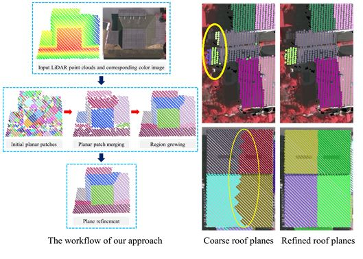
- We propose a new region growing-based coarse roof plane segmentation approach. It generates the rough planar clusters via an octree-based method, and merges them using a hierarchical clustering method. The merged patches are selected as the robust seeds for region growing.
- We propose a novel boundary relabeling-based roof plane refinement strategy to improve the quality of the initial coarse plane input. We formulate the roof plane refinement as an energy maximization problem and optimize it using boundary relabeling, which is more efficient than the global energy optimization approach [15]. It can remove most of the errors existed in the coarse segmentation and significantly improve the accuracy of the boundaries between adjacent roof planes.
2. Region Growing-Based Coarse Roof Plane Segmentation
| Algorithm 1 Region growing-based coarse roof plane segmentation |
| Input: The input building point clouds . Output: The coarse roof planes .
|
2.1. Octree-Based Rough Planar Patch Extraction
2.2. Planar Patch Merging Using Hierarchical Clustering
2.3. Point-Based Region Growing
3. Roof Plane Refinement
3.1. Plane Refinement as an Energy Maximization
3.1.1. Distance Term
3.1.2. Boundary Term
3.2. Energy Optimization via Boundary Relabeling
4. Experimental Results and Discussion
4.1. Evaluation Metrics
4.2. Choice of Parameters
4.3. Comparative Evaluation
5. Conclusions
Author Contributions
Funding
Acknowledgments
Conflicts of Interest
References
- Chen, D.; Zhang, L.; Li, J.; Liu, R. Urban building roof segmentation from airborne LiDAR point clouds. Int. J. Remote Sens. 2012, 33, 6497–6515. [Google Scholar] [CrossRef]
- Awrangjeb, M.; Gilani, S.A.N.; Siddiqui, F.U. An effective data-driven method for 3-D building roof reconstruction and robust change detection. Remote Sens. 2018, 10, 1512. [Google Scholar] [CrossRef]
- Liu, X.; Zhang, Y.; Ling, X.; Wan, Y.; Liu, L.; Li, Q. TopoLAP: Topology recovery for building reconstruction by deducing the relationships between linear and planar primitives. Remote Sens. 2019, 11, 1372. [Google Scholar] [CrossRef]
- Li, M.; Rottensteiner, F.; Heipke, C. Modelling of buildings from aerial LiDAR point clouds using TINs and label maps. ISPRS J. Photogramm. Remote Sens. 2019, 154, 127–138. [Google Scholar] [CrossRef]
- Kahaki, S.M.M.; Nordin, M.J.; Ashtari, A.H. Contour-based corner detection and classification by using mean projection transform. Sensors 2014, 14, 4126–4143. [Google Scholar] [CrossRef] [PubMed]
- Im, J.H.; Im, S.H.; Jee, G.I. Vertical corner feature based precise vehicle localization using 3D LiDAR in urban area. Sensors 2016, 16, 1268. [Google Scholar] [CrossRef]
- Hackel, T.; Wegner, J.D.; Schindler, K. Contour detection in unstructured 3D point clouds. In Proceedings of the IEEE Conference on Computer Vision and Pattern Recognition, Las Vegas, NV, USA, 26 June–1 July 2016; pp. 1610–1618. [Google Scholar]
- Melzer, T. Non-parametric segmentation of ALS point clouds using mean shift. J. Appl. Geod. 2007, 1, 159–170. [Google Scholar] [CrossRef]
- Filin, S.; Pfeifer, N. Segmentation of airborne laser scanning data using a slope adaptive neighborhood. ISPRS J. Photogramm. Remote Sens. 2006, 60, 71–80. [Google Scholar] [CrossRef]
- Kong, D.; Xu, L.; Li, X.; Li, S. K-plane-based classification of airborne LiDAR data for accurate building roof measurement. IEEE Trans. Instrum. Meas. 2014, 63, 1200–1214. [Google Scholar] [CrossRef]
- Biosca, J.; Lerma, J. Unsupervised robust planar segmentation of terrestrial laser scanner point clouds based on fuzzy clustering methods. ISPRS J. Photogramm. Remote Sens. 2008, 63, 84–98. [Google Scholar] [CrossRef]
- Sampath, A.; Shan, J. Segmentation and reconstruction of polyhedral building roofs from aerial LiDAR point clouds. IEEE Trans. Geosci. Remote Sens. 2009, 48, 1554–1567. [Google Scholar] [CrossRef]
- Vo, A.V.; Truong-Hong, L.; Laefer, D.F.; Bertolotto, M. Octree-based region growing for point cloud segmentation. ISPRS J. Photogramm. Remote Sens. 2015, 104, 88–100. [Google Scholar] [CrossRef]
- Zhang, C.; He, Y.; Fraser, C.S. Spectral clustering of straight-line segments for roof plane extraction from airborne LiDAR point clouds. IEEE Geosci. Remote Sens. Lett. 2018, 15, 267–271. [Google Scholar] [CrossRef]
- Yan, J.; Shan, J.; Jiang, W. A global optimization approach to roof segmentation from airborne LiDAR point clouds. ISPRS J. Photogramm. Remote Sens. 2014, 94, 183–193. [Google Scholar] [CrossRef]
- Duda, R.; Hart, P. Use of the Hough transformation to detect lines and curves in pictures. Commun. ACM 1972, 15, 11–15. [Google Scholar] [CrossRef]
- Fischler, M.A.; Bolles, R.C. Random sample consensus: A paradigm for model fitting with applications to image analysis and automated cartography. Commun. ACM 1981, 24, 381–395. [Google Scholar] [CrossRef]
- Vosselman, G.; Gorte, B.; Sithole, G.; Rabbani, T. Recognising structure in laser scanner point clouds. Int. Arch. Photogramm. Remote Sens. Spat. Inf. Sci. 2004, 46, 33–38. [Google Scholar]
- Borrmann, D.; Elseberg, J.; Lingemann, K.; Nüchter, A. The 3D Hough transform for plane detection in point clouds: A review and a new accumulator design. 3D Res. 2011, 2, 3. [Google Scholar] [CrossRef]
- Hulik, R.; Spanel, M.; Smrz, P.; Materna, Z. Continuous plane detection in point-cloud data based on 3D Hough transform. J. Vis. Commun. Image Represent. 2014, 25, 86–97. [Google Scholar] [CrossRef]
- Tian, Y.; Song, W.; Chen, L.; Sung, Y.; Kwak, J.; Sun, S. Fast planar detection system using a GPU-based 3D Hough transform for LiDAR point clouds. Appl. Sci. 2020, 10, 1744. [Google Scholar] [CrossRef]
- Nguyen, A.; Le, B. 3D point cloud segmentation: A survey. In Proceedings of the IEEE Conference on Robotics, Automation and Mechatronics, Manila, Philippines, 12–15 November 2013. [Google Scholar]
- Kahaki, S.M.; Wang, S.L.; Stepanyants, A. Accurate registration of in vivo time-lapse images. In Proceedings of the Medical Imaging 2019: Image Processing, San Diego, CA, USA, 16–21 February 2019. [Google Scholar]
- Tarsha-Kurdi, F.; Landes, T.; Grussenmeyer, P. Hough-transform and extended RANSAC algorithms for automatic detection of 3D building roof planes from LiDAR data. Int. Arch. Photogramm. Remote Sens. 2007, 66, 124–132. [Google Scholar]
- Xu, B.; Jiang, W.; Shan, J.; Zhang, J.; Li, L. Investigation on the weighted RANSAC approaches for building roof plane segmentation from LiDAR point clouds. Remote Sens. 2016, 8, 5. [Google Scholar] [CrossRef]
- Li, L.; Yang, F.; Zhu, H.; Li, D.; Li, Y.; Tang, L. An improved RANSAC for 3D point cloud plane segmentation based on normal distribution transformation cells. Remote Sens. 2017, 9, 433. [Google Scholar] [CrossRef]
- Canaz Sevgen, S.; Karsli, F. An improved RANSAC algorithm for extracting roof planes from airborne LiDAR data. Photogramm. Rec. 2019. [Google Scholar] [CrossRef]
- Dal Poz, A.P.; Yano Ywata, M.S. Adaptive random sample consensus approach for segmentation of building roof in airborne laser scanning point cloud. Int. J. Remote Sens. 2020, 41, 2047–2061. [Google Scholar] [CrossRef]
- Gorte, B. Segmentation of TIN-structured surface models. Int. Arch. Photogramm. Remote Sens. Spat. Inf. Sci. 2002, 34, 465–469. [Google Scholar]
- Zhang, K.; Yan, J.; Chen, S.C. Automatic construction of building footprints from airborne LiDAR data. IEEE Trans. Geosci. Remote Sens. 2006, 44, 2523–2533. [Google Scholar] [CrossRef]
- Cao, R.; Zhang, Y.; Liu, X.; Zhao, Z. Roof plane extraction from airborne LiDAR point clouds. Int. J. Remote Sens. 2017, 38, 3684–3703. [Google Scholar] [CrossRef]
- Xu, Y.; Yao, W.; Hoegner, L.; Stilla, U. Segmentation of building roofs from airborne LiDAR point clouds using robust voxel-based region growing. Remote Sens. Lett. 2017, 8, 1062–1071. [Google Scholar] [CrossRef]
- Deschaud, J.E.; Goulette, F. A fast and accurate plane detection algorithm for large noisy point clouds using filtered normals and voxel growing. In Proceedings of the International Symposium on 3DPVT, Paris, France, 17–20 May 2010. [Google Scholar]
- Gilani, S.A.N.; Awrangjeb, M.; Lu, G. Segmentation of airborne point cloud data for automatic building roof extraction. GISci. Remote Sens. 2018, 55, 63–89. [Google Scholar] [CrossRef]
- Wu, T.; Hu, X.; Ye, L. Fast and accurate plane segmentation of airborne LiDAR point cloud using cross-line elements. Remote Sens. 2016, 8, 383. [Google Scholar] [CrossRef]
- Awrangjeb, M.; Fraser, C. An automatic and threshold-free performance evaluation system for building extraction techniques from airborne LiDAR data. IEEE J. Sel. Top. Appl. Earth Obs. Remote Sens. 2014, 7, 4184–4198. [Google Scholar] [CrossRef]
- Feng, C.; Taguchi, Y.; Kamat, V.R. Fast plane extraction in organized point clouds using agglomerative hierarchical clustering. In Proceedings of the IEEE International Conference on Robotics and Automation (ICRA), Hong Kong, China, 31 May–7 June 2014. [Google Scholar]
- Van den Bergh, M.; Boix, X.; Roig, G.; de Capitani, B.; Van Gool, L. Seeds: Superpixels extracted via energy-driven sampling. In Proceedings of the European Conference on Computer Vision (ECCV), Florence, Italy, 7–13 October 2012. [Google Scholar]
- Woo, K.; Kang, E.; Wang, S.; Lee, K.H. A new segmentation method for point cloud data. Int. J. Mach. Tools Manuf. 2002, 42, 167–178. [Google Scholar] [CrossRef]
- Wang, M.; Tseng, Y. Automatic segmentation of LiDAR data into coplanar point clusters using an octree-based split-and-merge algorithm. Photogramm. Eng. Remote Sens. 2010, 76, 407–420. [Google Scholar] [CrossRef]
- Yao, J.; Taddei, P.; Ruggeri, M.R.; Sequeira, V. Complex and photo-realistic scene representation based on range planar segmentation and model fusion. Int. J. Robot. Res. 2011, 30, 1263–1283. [Google Scholar] [CrossRef]
- Rabbani, T.; Van Den Heuvel, F.; Vosselman, G. Segmentation of point clouds using smoothness constraints. In Proceedings of the ISPRS Commission V Symposium: Image Engineering and Vision Metrology, Dresden, Germany, 25–27 September 2006. [Google Scholar]
- Cramer, M. The DGPF-test on digital airborne camera evaluation–overview and test design. Photogramm. Fernerkund. Geoinf. 2010, 2010, 73–82. [Google Scholar] [CrossRef]
- Schnabel, R.; Wahl, R.; Klein, R. Efficient RANSAC for point-cloud shape detection. Comput. Graph. Forum 2007, 26, 214–226. [Google Scholar] [CrossRef]
- Shan, J.; Lee, S. Quality of building extraction from IKONOS imagery. J. Surv. Eng. 2005, 131, 27–32. [Google Scholar] [CrossRef]
- Estrada, F.; Jepson, A. Benchmarking image segmentation algorithms. Int. J. Comput. Vis. 2009, 85, 167–181. [Google Scholar] [CrossRef]
- Kahaki, S.M.M.; Nordin, M.J.; Ashtari, A.H.; Zahra, S.J. Invariant feature matching for image registration application based on new dissimilarity of spatial features. PLoS ONE 2016, 11, e0149710. [Google Scholar]


| Vaihingen Dataset | Wuhan Dataset | |
|---|---|---|
| Location | Vaihingen (Germany) | Wuhan (China) |
| Laser scanner | Leica ALS50 | Trimble Harrier 68i |
| Point density | 4 points/m | 8 points/m |
| Roof type | Mostly gable roof with a large slope | Flat roof and gable roof |
| Description of the study areas | Small-sized and detached buildings with complex roof structure | Large-sized buildings with complex roof structure |
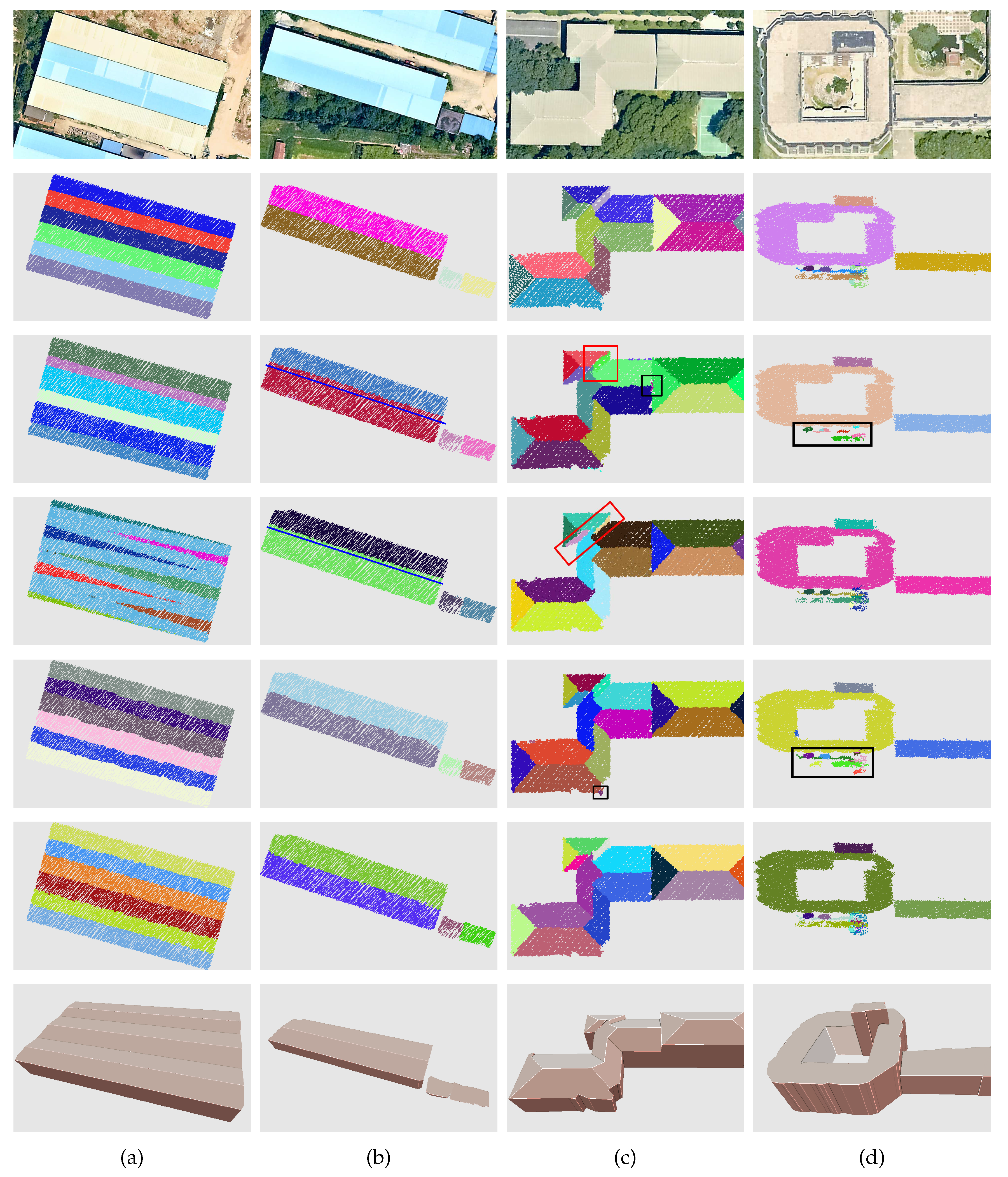
| Figure 6a | Time(s) | ||||||||||||
| RG | 63 | 58 | 5 | 15 | 92.06 | 79.45 | 74.36 | 22.22 | 5.48 | 76.07 | 84.19 | 79.92 | 0.17 |
| RANSAC | 63 | 57 | 6 | 23 | 90.48 | 71.25 | 66.28 | 20.63 | 5.00 | 75.57 | 82.76 | 79.00 | 0.91 |
| GO | 63 | 61 | 2 | 14 | 96.83 | 81.33 | 79.22 | 17.46 | 1.33 | 81.26 | 92.38 | 86.46 | 11.55 |
| BR | 63 | 60 | 3 | 6 | 95.24 | 90.91 | 86.96 | 6.35 | 3.03 | 86.50 | 92.76 | 89.52 | 0.52 |
| Figure 6b | |||||||||||||
| RG | 40 | 39 | 1 | 11 | 97.50 | 78.00 | 76.47 | 12.50 | 4.00 | 88.76 | 88.29 | 88.52 | 0.16 |
| RANSAC | 40 | 38 | 2 | 6 | 95.00 | 86.36 | 82.61 | 10.00 | 4.55 | 89.92 | 90.92 | 90.42 | 0.93 |
| GO | 40 | 39 | 1 | 3 | 97.50 | 92.86 | 90.70 | 5.00 | 0.00 | 93.65 | 95.53 | 94.58 | 9.37 |
| BR | 40 | 40 | 0 | 1 | 100.00 | 97.56 | 97.56 | 2.50 | 0.00 | 95.52 | 96.24 | 95.88 | 0.38 |
| Figure 7a | |||||||||||||
| RG | 68 | 64 | 4 | 31 | 94.12 | 67.37 | 64.65 | 29.41 | 13.68 | 48.64 | 55.56 | 51.87 | 1.17 |
| RANSAC | 68 | 58 | 10 | 17 | 85.29 | 77.33 | 68.24 | 32.35 | 13.33 | 47.29 | 53.06 | 50.01 | 1.81 |
| GO | 68 | 67 | 1 | 4 | 98.53 | 94.37 | 93.06 | 5.88 | 2.82 | 79.09 | 81.66 | 80.35 | 99.86 |
| BR | 68 | 67 | 1 | 3 | 98.53 | 95.71 | 94.37 | 2.94 | 1.43 | 86.61 | 85.42 | 86.01 | 3.96 |
| Figure 7b | |||||||||||||
| RG | 86 | 74 | 12 | 83 | 86.05 | 47.13 | 43.69 | 25.58 | 3.82 | 52.63 | 54.32 | 53.46 | 1.65 |
| RANSAC | 86 | 78 | 8 | 35 | 90.70 | 69.03 | 64.46 | 13.95 | 7.96 | 68.71 | 73.94 | 71.23 | 2.23 |
| GO | 86 | 79 | 7 | 62 | 91.86 | 56.03 | 53.38 | 19.77 | 2.13 | 67.57 | 78.15 | 72.48 | 390.25 |
| BR | 86 | 80 | 6 | 1 | 93.02 | 98.77 | 91.95 | 1.16 | 4.94 | 88.76 | 85.92 | 87.32 | 5.21 |
© 2020 by the authors. Licensee MDPI, Basel, Switzerland. This article is an open access article distributed under the terms and conditions of the Creative Commons Attribution (CC BY) license (http://creativecommons.org/licenses/by/4.0/).
Share and Cite
Li, L.; Yao, J.; Tu, J.; Liu, X.; Li, Y.; Guo, L. Roof Plane Segmentation from Airborne LiDAR Data Using Hierarchical Clustering and Boundary Relabeling. Remote Sens. 2020, 12, 1363. https://doi.org/10.3390/rs12091363
Li L, Yao J, Tu J, Liu X, Li Y, Guo L. Roof Plane Segmentation from Airborne LiDAR Data Using Hierarchical Clustering and Boundary Relabeling. Remote Sensing. 2020; 12(9):1363. https://doi.org/10.3390/rs12091363
Chicago/Turabian StyleLi, Li, Jian Yao, Jingmin Tu, Xinyi Liu, Yinxuan Li, and Lianbo Guo. 2020. "Roof Plane Segmentation from Airborne LiDAR Data Using Hierarchical Clustering and Boundary Relabeling" Remote Sensing 12, no. 9: 1363. https://doi.org/10.3390/rs12091363
APA StyleLi, L., Yao, J., Tu, J., Liu, X., Li, Y., & Guo, L. (2020). Roof Plane Segmentation from Airborne LiDAR Data Using Hierarchical Clustering and Boundary Relabeling. Remote Sensing, 12(9), 1363. https://doi.org/10.3390/rs12091363