Remote Sensing of Boreal Wetlands 1: Data Use for Policy and Management

Abstract

Wetlands have and continue to undergo rapid environmental and anthropogenic modification and change to their extent, condition, and therefore, ecosystem services. In this first part of a two-part review, we provide decision-makers with an overview on the use of remote sensing technologies for the ‘wise use of wetlands’, following Ramsar Convention protocols. The objectives of this review are to provide: (1) a synthesis of the history of remote sensing of wetlands, (2) a feasibility study to quantify the accuracy of remotely sensed data products when compared with field data based on 286 comparisons found in the literature from 209 articles, (3) recommendations for best approaches based on case studies, and (4) a decision tree to assist users and policymakers at numerous governmental levels and industrial agencies to identify optimal remote sensing approaches based on needs, feasibility, and cost. We argue that in order for remote sensing approaches to be adopted by wetland scientists, land-use managers, and policymakers, there is a need for greater understanding of the use of remote sensing for wetland inventory, condition, and underlying processes at scales relevant for management and policy decisions. The literature review focuses on boreal wetlands primarily from a Canadian perspective, but the results are broadly applicable to policymakers and wetland scientists globally, providing knowledge on how to best incorporate remotely sensed data into their monitoring and measurement procedures. This is the first review quantifying the accuracy and feasibility of remotely sensed data and data combinations needed for monitoring and assessment. These include, baseline classification for wetland inventory, monitoring through time, and prediction of ecosystem processes from individual wetlands to a national scale.

1. Introduction

Wetland processes include hydrological water cycling and biogeochemical processes, both of which maintain wetland function, carbon storage and methane emission, biological productivity, and wetland habitats, as described by the Ramsar Convention on Wetlands. As part of these abiotic and biotic processes, a range of ecosystem services are provided that are beneficial to human populations through local economy, and sustainability and resilience of communities [1]. These include provisioning services (food, freshwater, fibre, and fuel), regulating services (climatic regulation, hydrological regulation, pollution control, erosion protection, and mitigation of natural hazards), cultural services (spiritual, educational, and religious), and supporting services (biodiversity, soil formation, and nutrient cycling). Wetlands provide more ecosystem services and are valued more highly than any other terrestrial ecosystem on Earth [1]. Detrimental changes in wetland extent and condition are therefore assumed to reduce ecosystem services and value [2]. For example, monetary losses associated with the global reduction of wetland area and cumulative ecosystem services between 1997 and 2011 was estimated to be approximately 10 trillion USD per year [1].

Anthropogenic modification and pressures on wetlands are increasing exponentially [2]. There is also a disconnect in understanding of wetland inventory, drivers of wetland change, and the integration of wetland value into policy and decision-making efforts by government and industry [3]. Wise management and use of wetlands require knowledge of the drivers of wetland changes that affect all levels and scales of ecosystem function. These include direct loss and degradation from drainage and land conversion, introduction of pollution and invasive species, and other human activities that affect water quality and frequency of flooding and drying. Indirect drivers of wetland change include climate change impacts and feedbacks, such as wildfires and drought, which are stochastic elements of ecosystem change.

Holistic understanding and quantification of the cumulative impacts on wetlands requires not only field assessment, but also the integration of modelling with remotely sensed data [4]. At the most basic level, remotely sensed data are used to quantify the extent of wetlands and open water areas over broad regions [5]. The accuracy of inventories of wetland area and type has improved drastically since the 1980’s due to developments in remote sensing technologies and analytical methods. Remote sensing is defined as the science of observing and recording information about objects from a distance, without touching them, often from airborne or spaceborne platforms, but can also include ground-based photography, imaging, and active survey (e.g., horizontally scanning lidar, radar). Remote sensing approaches are also used to assess wetland ecosystem changes in area extent and condition over time.

Field data collection has traditionally been used for thorough identification of local wetland changes in processes over time. Ground-based information is necessary for understanding the impacts of drivers but is often limited in area extent (local scale) and temporal coverage (visits per year and total years monitored). For instance, academic field-based research initiatives typically progress through funding cycles of three to five years. Similar timelines occur for government scientists associated with changing government administrations and changing priorities. On the other hand, data acquisition by satellites occur up to several times per week and over periods of years to decades, which are then used to identify changes in the environment at local to national scales. Changes in wetland condition, for example, can be determined through the analysis of spatial variations in the colour and texture of vegetation, moisture characteristics, or surface water. By including multiple images, one may identify indicators of cumulative drivers of wetland condition through changes in vegetation structure and hydrological regime, which alter the colour and texture of images over time.

Remote sensing is also used to improve model outputs through parameterisation and/or evaluation of one or more input drivers. The combination of the two (remote sensing and modelling) influence decision-making processes because they include both the spatial and contextual/proximal dynamics, which could be used to inform management decisions for up to thousands of wetland ecosystems. The combination of remotely sensed and field data collections are imperative for quantifying direct and indirect drivers of wetland ecosystem change, implications to ecosystem services, and mitigation of wetland disturbance. Despite this, there needs to be an explicit treatment of the methods of wetland classification and how these classes are used to inform wetland value to support decision-making procedures from local to federal levels of government (Figure 1). Such frameworks currently do not exist in Canada nor in many other jurisdictions or countries.

Government agencies are exploring the utility of remotely sensed data within operational wetland management and monitoring frameworks to improve the accuracy of baseline wetland inventory data and knowledge of drivers of wetland ecosystem change. The desire is to improve wetland management decisions and outcomes, however, slow adoption of procedures and practices often over many years is due in part to the technical nature of remote sensing and the complexity of wetland science. This includes a wide range of wetland applications and monitoring needs, various remote sensing technologies used, and differences in the way in which data are collected, analysed, and compared. While there have been numerous technical reviews on the use of remotely sensed data for characterising wetlands, no study has provided scientists and decision-makers with a range of accuracies that can be expected across wetland application areas. Because of this, standard procedures for incorporating remotely sensed data into monitoring programs have not been implemented and the use of remote sensing often remains ad hoc or for scientific/academic purposes.

To address these issues, this manuscript (Part 1 of a two-part series, both in this edition) provides a statistically based assessment of the range of accuracies of remotely sensed data and derivative products compared with field data, as determined from the literature. While this is not a thorough review of optimal data analysis procedures (these are examined in Part 2), this will provide decision-makers with a basic understanding of accuracy expectations and feasibility if remotely sensed data are included within a wetland management framework. Feasibility is defined here as the expected accuracy and applicability of remote sensing technologies, including cost and scale (or minimum mapping unit) requirements needed to infer spatio-temporal wetland attributes and ‘no net loss’ requirements [2].

Part 1 focuses on four key objectives: Objective (1) a synthesis of the history of remote sensing over the last 50+ years for examining wetland extent, inventory, and processes of importance described in the Ramsar Convention on Wetlands [2]; Objective (2) a feasibility study on the use of remotely sensed data products compared with field data, determined from reported accuracies from 209 peer-reviewed journal articles; Objective (3) recommendations for best approaches for the use of remote sensing within an inventory and monitoring framework using boreal region case studies, where available. Finally, Objective (4) a decision tree diagram and table to enable decision-makers to choose optimal remote sensing approaches based on user needs, feasibility, and cost. This review provides an explicit framework for the use of remotely sensed data for wetland monitoring in support of policy and decision-making requirements within different levels of government and industry (Figure 1). In Part 2, we provide a review of best practices for the most accurate assessment of wetlands and their functions. Our review is broadly addressed to decision-makers interested in the ‘wise use of wetlands’ and is relevant for global wetland management and monitoring using remotely sensed data analytics. Both parts of this compendium focus on boreal-region wetlands and peatlands, primarily from a Canadian perspective, however, we broadly assessed and recommended analytical remote sensing methods using examples from global inland and coastal wetlands, where they have not been used in a boreal context, to ensure our review was far-reaching and comprehensive.

2. Objective 1: History and Uses of Remote Sensing of Wetland Ecosystems

The science of remote sensing, in combination with knowledge from wetland sciences, is now, more than ever, well-positioned to accurately quantify wetland extent, wetland condition, and the changes in these attributes over time (addressed in Part 2). As such, remote sensing science has rapidly expanded the capability to assess wetlands due to three key developments: (i) Global satellite data coverage from Landsat series (1972 to current; National Aeronautics and Space Administration, NASA) and now Sentinel (2014 to current; Copernicus Programme) are freely available. This has enabled broad-area mapping of wetlands in both developed and developing countries, and the proliferation of new methodologies to examine remotely sensed data. (ii) The breadth of wetland attributes measured using remote sensing technology have increased dramatically in recent years, given advancements in new technologies such as multi-spectral sensors (e.g., Sentinel-2) and multi-spectral lidar, computing power and methods, and improved fidelity of spatial data products over time. (iii) Methodological developments and the fusion of multi-disciplinary research have improved the integration of remotely sensed data, field data, and modelling to measure proxy indicators of underlying processes related to ecosystem condition and change over time. Historic use of airborne and satellite remote sensing systems often used for studying the land surface through time, including wetlands, are introduced in Figure 2. Single and multiple acquisition aerial photography have been used to characterise the earth’s surface at a ‘snapshot’ in time since the 1940’s. The development of numerous optical (multi-spectral and hyperspectral) remote sensing platforms accelerated during the mid to late 1980’s and into the 1990’s (Figure 2). Single acquisition airborne hyperspectral remote sensing systems became popular during the 1990’s followed by Synthetic Aperture Radar (SAR) and airborne lidar from 2000, especially towards the beginning of the 21st century.

Interestingly, the use of remotely sensed data for estimating wetland extent and type, according to the Ramsar Convention on Wetlands [2], was relatively limited until about 2003 (Figure 3). This may be due to a lack of interest in wetland environments compared with forests owing to their supposed low ‘value’, whereby forest merchantable biomass was considered of high value (F. Ahern, personal communication). By 2013, increasing research activities included data conflation, also known as fusion. Conflation refers to the use of two or more remote sensing and geospatial datasets based on their strengths so as to reduce redundant information.

Most early articles (~1973 to 1997) using remotely sensed data to study wetlands were published in ecosystem process journals that were not dedicated to the study of remote sensing methods’ development. Early articles focused on wetland mapping and characterisation using aerial photography [6,7,8,9,10,11] or the use of chronosequence air photos to track wetland change [12,13,14]. Validation of wetland extent and locational features using the civilian global positioning system (GPS) did not occur at most sites until after May 2000, when Selective Availability of GPS satellites was turned off. Up to that time, coarser resolution remotely sensed data products were often compared with delineated air photos as validation (e.g., References [15,16]).

In 2002, Ozesmi and Bauer [17] wrote a seminal review of the use of remote sensing for the study of wetlands, but it was not until early December 2008 that all Landsat data became freely available on a United States Geological Survey (USGS) online archive, contributing to accelerated use of Landsat data for monitoring wetland (and broader ecosystem) changes over time [18,19]. Later on, increasingly complex methods and comparisons warranted publication in remote sensing or information system and computer science journals [20,21] (Figure 3). These were added to the body of literature at the exponential rate of growth observed in Figure 3 (k = 0.07, R² = 0.53, where k is the growth constant, or the frequency of growth over a period of time and R² refers to the coefficient of determination for an exponential model). Publication of articles in ecosystem science journals also increased exponentially, but at a reduced rate (k = 0.04, R² = 0.52, for a similar exponential model). Additional sensors, including RADARSAT-2, which followed the success of RADARSAT-1, and lidar became operationalized through the late 2000’s (Figure 2). These sensors were also important contributors to application development important for wetland characterisation, including water extent and hydro-period [22,23], and topography and vegetation structure [24,25,26,27].

Remote sensing offers non-invasive methods for collecting information using either ‘passive’ or ‘active’ observation approaches. Passive sensors detect electromagnetic radiation emitted from the sun that is absorbed, transmitted, or reflected from or through objects on the Earth’s surface (similar to a photograph). The ability of objects to absorb, emit, transmit, or reflect radiation depends on a combination of structural and biochemical attributes and the combined distribution of objects within a pixel [28]. Multispectral remote sensing detects energy variations across several discrete wavelengths or ‘bands’, while hyperspectral remote sensing can detect energy variations across several hundred discrete bands, thereby providing even more information on structure and biochemistry (e.g., nitrogen, water content) (e.g., Reference [29]). Advantages of passive remote sensing include potentially: long time series (e.g., long-term USGS and NASA investment in AVHRR, Landsat, and MODIS) and up to multiple acquisitions per week, inexpensive data collection (low to moderate resolution satellites), and ease of application. However, these datasets, often with low spatial resolution data (>10 × 10 m pixels), may not accurately capture wetland transition areas and edges due to mixed pixels (pixels containing heterogeneous land covers or characteristics), resulting in uncertainty in changes of wetland extent.

Active sensors provide their own energy source by directing radiation towards a target and measuring the properties of energy received. For example, airborne lidar systems rapidly emit laser pulses (up to ~1,000,000 pulses per second) within one or more discrete wavelengths and measure the timing between laser pulse emission and reception, and the intensity or amount of energy of the reflected laser pulse [30]. Lidar is able to detect vegetation structural characteristics (e.g., References [24,26]) and ground surface elevation (e.g., References [26,31]) at high spatial resolution (typically one to tens of laser pulse reflections per square meter). SAR emits and receives radio waves. The polarisation of wave emission (either vertical or horizontal) allows differentiation of textural and moisture attributes of the target related to its dielectric properties [32,33]. Therefore, SAR is particularly useful for detecting variations in backscattered energy related to surface soil moisture characteristics, surface water, and inundated emergent vegetation (e.g., Reference [34]). Advantages of active remote sensing include potentially high spatial resolution and the capability to operate independently of natural light sources, therefore offering less restricted operating times (i.e., active sensors can be operated day or night and in the case of SAR, through clouds), but without broad area coverage [5]. Manufacturers may also tailor the emitted radiation to specific applications; for example, avoiding red wavelengths for the sensing of green vegetation as the majority of the emitted radiation will be absorbed by such targets. This capability has numerous secondary advantages such as altering the emission wavelengths so that clouds become transparent and providing the ability to penetrate above-ground features such as vegetation, allowing the retrieval of structural characteristics. Disadvantages of active remote sensing include cost of data acquisition depending on platform, though Sentinel-1 is freely available and RADARSAT series costs are reduced by subsidies from the Canadian Government. In addition, active remote sensing also may require advanced expertise and software tools and requires targeted planning of data collections and acquisition.

The combination of active and passive sensors within a range of spectral, spatial, and temporal resolutions, and the ability to develop complimentary data information, has also increased the variety of wetland data products derived (e.g., References [35,36,37]) using data conflation frameworks. The combination of information streams from different sensors has allowed users to characterise wetland attributes that may be difficult to identify using single sensors. For example, the authors of Reference [38] were able to identify ephemeral vernal pools by combining PALSAR L-band SAR, laser return intensity from lidar data, and a Digital Elevation Model (DEM). In another study [39], vernal pools were identified using colour infrared aerial photography and lidar data. Typically, vernal pools are difficult to identify using single remote sensing technologies and therefore many of these are missed within wetland classifications [40]. This is due to occlusion of the ground surface by tree canopies, particularly problematic for optical imagery but can be sensed using lidar, an inability to quantify standing water within vernal pools using lidar data, observed using SAR, and an inability of lidar and SAR for measuring tree species and texture, which can be mapped using optical imagery. Combining sensors using data conflation methods improves the accuracy with which these are identified [38]. Other examples include: peatland microtopographic and moss species monitoring using a hydrological framework based on high spatial resolution lidar and IKONOS optical imagery [41], classification of bogs and fens using RADARSAT-2 with quad-polarimetry and Landsat OLI multi-spectral imagery within an object-based image analysis framework [42], invasive species identification using multiple spectral imagers such as MIVIS, AISA Systems, GeoEye, and Worldview-2 [43], and overland flooding using a combination of Landsat TM, SPOT, and RADARSAT-1 [44], among others. With increased data availability and long-term data acquisition periods [45] (Figure 2), data conflation has become the state-of-the-art in remote sensing wetland science.

When comparing costs associated with field data collection, the average cost of acquisition and processing of lidar data per acre of forest land is comparable to field data collection, estimated at 2.63 USD, for continuous collection of forest attributes. Forest inventory of tree structure: basal area, density, and height, is estimated to be 2.46 USD, however these are for individual plots within a forest management area [46]. Cost of wetland inventory, especially in remote areas, is likely to be much higher, though areas measured may be smaller (described in Part 2).

Table 1. Historical to current remote sensing derivative products, classes, and descriptions used to study boreal wetland ecosystems within the context of the Ramsar Convention. Ramsar Convention processes of interest for wetlands examined in the Table are divided into: Applications of Interest or wetland monitoring subjects of interest, derivative products, which can be derived from remote sensing data to support applications, descriptions of the derivative products produced by remotely sensed data, and References that have developed methods and derivative products using different remote sensing systems. References are used in comparisons in Figure 4, Figure 5 and Figure 6.

Ramsar Process	Applications of Interest	Derivative Products	Description	Remote Sensing Systems	References
Wetland extent	Landcover	Landcover class	General land cover classes, where wetlands are one of many land cover classes characterised by remotely sensed data	Air photos, MIVIS, AVIRIS, Hyperion, Worldview, Quickbird, IKONOS, KOMPSAT, SPOT, Sentinel-2, Landsat, MODIS, AVHRR, RADARSAT, MERIS, NISAR, Sentinel-1, JERS, PALSAR, ERS 1, 2, SIR, Lidar	[6,12,15,36,47,48,49,50,51,52,53,54,55,56,57,58,59,60,61,62,63,64,65,66,67,68,69,70,71,72,73,74,75,76,77]
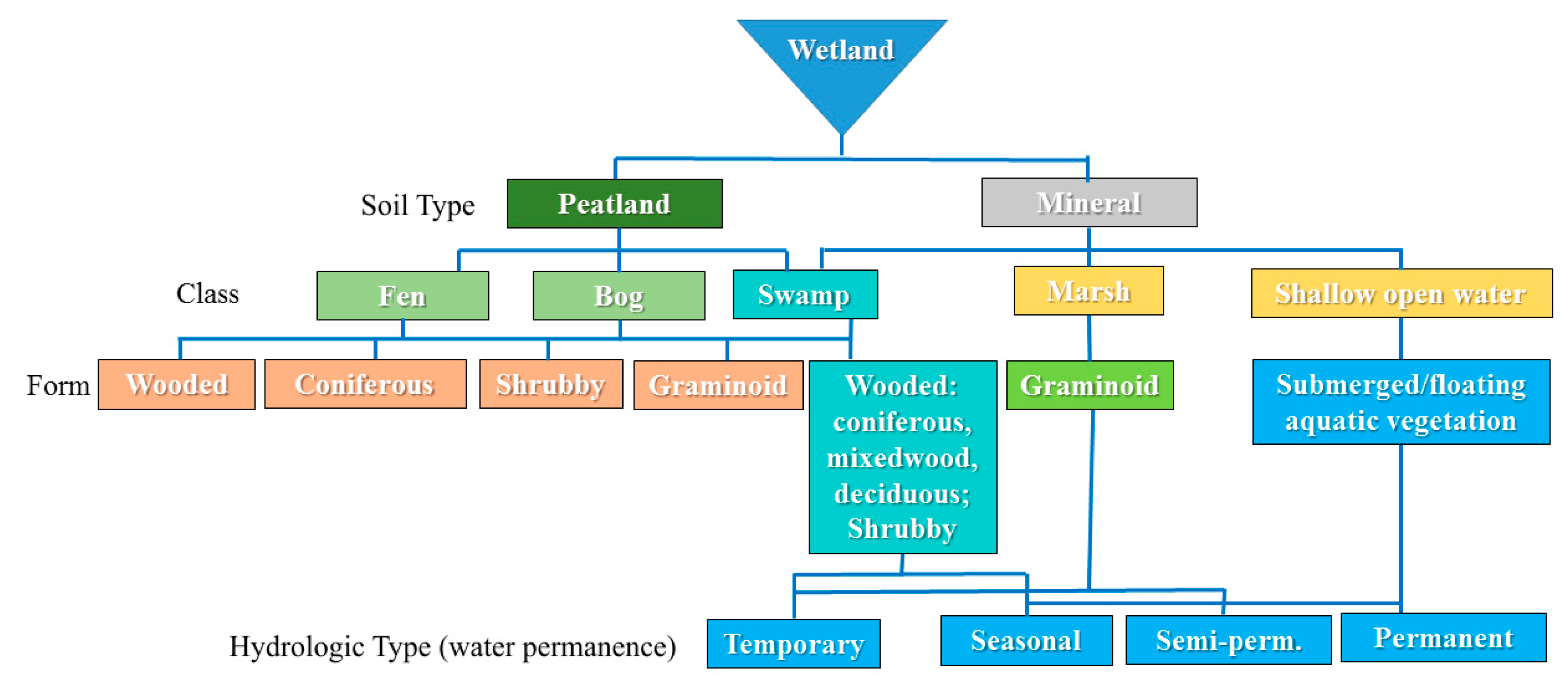
	Wetland class	Wetland class (e.g., Bog, Fen, Swamp, Marsh, Shallow open water) Wetland form structure including graminoid, shrubby, treed Wetland edge detection	More specific use of remote sensing data for classifying wetland class, physiognomic vegetation form, and accuracy of extent, including wetland edge detection	Air photos, Hymap, CASI, Worldview, Pleiades, Quickbird, IKONOS, RapidEye, SPOT, Landsat, MODIS, RADARSAT, PALSAR, ERS 1, 2, SeaSat SIR, Lidar	[7,10,11,19,35,36,38,40,41,42,47,50,57,63,70,72,76,78,79,80,81,82,83,84,85,86,87,88,89,90,91,92,93,94,95,96,97,98,99,100,101,102,103,104,105,106,107,108,109,110,111,112,113,114]
	Vegetation species	Tree/shrub/graminoid (etc.) species identification; invasive species Moss/ground cover identification	Identification of vegetation species and ground covers, variability, and extent	Air photo, PROBE, MIVIS, ROSIS, Hymap, CASI, AVIRIS, Hyperion, Worldview, Quickbird, IKONOS, SPOT, Sentinel-2, Landsat, TerraSAR-X, Lidar	[9,10,11,15,16,19,41,43,44,60,69,70,72,76,82,102,103,104,105,106,107,108,109,110,112,113,114,115,116,117,118,119,120,121,122,123,124,125,126,127,128,129,130,131,132,133,134,135,136,137,138,139,140,141]
	Ecosystem change	Ecosystem change Restoration Reclamation	Change of wetland ecosystems over time, including expansion and contraction of wetland land covers, changes in species. Requires accuracy standards for wetland class to determine accuracy of wetland change	Airphotos, Quickbird, IKONOS, SPOT, Landsat, MODIS, AVHRR, Lidar	[12,19,44,71,142,143,144,145,146,147,148,149,150,151,152,153,154,155]
Biological Productivity	Ecosystem productivity	Productivity, biomass Carbon and methane Foliage biogeo-chemistry	Indicators of vegetation productivity, vegetation indices; Leaf biogeochemistry (e.g., N) often measured using hyperspectral remote sensing	Hymap, CASI, Hyperion, Worldview, Rapideye, Sentinel-2, Landsat, MODIS, MERIS, Sentinel-1, SMAP, Lidar	[21,134,146,154,156,157,158,159,160,161,162,163,164,165,166,167,168]
	Vegetation structure	Vegetation structure Friction Stress	Measurement of structural and foliage attributes of vegetation; Frictional components of land and vegetation for flood extent mapping and air movement; Variations in structure associated with stress	AVIRIS, IKONOS, Landsat, MODIS, Lidar	[21,26,112,128,169,170,171]
	Habitat	Fauna Insect	Habitat characterisation for fauna and insects	Air photo, GeoSAT, IKONOS, Landsat, MODIS, Lidar	[72,130,131,155,160,172,173,174,175]
	Wildfire effects	Fire impacts Loss of biomass Fire severity	Post-fire ecosystem changes, burn severity often determined from spectral burn indices, lidar	IKONOS, Sentinel-1, 2, Landsat, RADARSAT, Lidar	[73,147,176]
Hydrological regime/water cycling	Water flux	Evapo-transpiration	Modelling water losses often based on structure/leaf area; measurement using thermal infrared imagery	Landsat, MODIS, AVHRR	[50,148,171,177,178,179]
	Water extent/level	Water extent Water level Bathymetry	Water extent can be used to determine water level with an accurate DEM, and hydroperiod; Bathymetry determined from bathymetric lidar	Air photo, Quickbird, Cubesat (etc.), RapidEye, SPOT, Landsat, Sentinel-2, Sentinel-1, RADARSAT, JERS, ENVISAT, Palsar, SeaSat, SIR, GeoSat, Jason, Lidar	[8,9,20,22,23,36,39,44,75,91,93,118,124,144,162,174,180,181,182,183,184,185,186,187,188,189,190,191,192,193,194,195,196,197,198,199,200,201,202,203]
	Soil moisture/ water table	Soil moisture Position of the water table Hydraulic gradient	Surface soil moisture, saturation associated with water table at the ground surface, and estimates of hydrological gradient between saturated surfaces	SASI, CASI, ASTER, ERS-1,2, SMAP, Lidar	[93,126,178,204,205,206,207]
	Topography	Topographic variability Wetland connectivity Erosion	Local topographic variations influencing distribution of soil moisture, vegetation species, structures, hydroperiod, contributing basin area, wetland hydrological connectivity, and water/nutrient flows	Worldview, Lidar	[26,27,128,155,207,208,209,210,211,212,213]
Biogeochemical processes	Water chemistry/turbidity	Trophic status Suspended sediment Turbidity/Secchi disk depth Salinity	Spectral reflection/absorption of water column constituents; Spectral indicators of saline soil surfaces	Air photos, MIVIS, Sentinel-2, Landsat, MODIS, MERIS, JERS-1	[124,154,191,214,215,216,217,218,219,220,221,222]
	Surface geology/soils	Surface geology Soils	Distribution of surface geological formations often based on DEM textural attributes and/or spectral characteristics of bare soils/rock	MIVIS, Lidar	[223,224]
	Mine spill detection	Oil spill detection Contaminants	Overland flow of oil spills and contaminants measured using optical/hyperspectral remote sensing	Air photos, AVIRIS, SPOT, Landsat	[152,225,226,227,228]
Climate Change	Climate forcing	Wetland class change	Broad area wetland class or characteristics (e.g., albedo) and implications for climate change	MODIS	[143,145,149,170,229]

SIR—Shuttle Imaging Radar.

provides an overview (chronologically where possible) of wetland-related products derived from remote sensing, as characterised by the four dominant wetland processes described by the Ramsar Convention on Wetlands [2], and in addition, wetland extent and climate change impacts.

3. Objective 2: Feasibility of Remotely Sensed Data Products for Wetland Applications

3.1. Approach

To determine the feasibility of remotely sensed data for wetland applications, we accessed articles that provided statistical comparisons (coefficient of determination or users’ accuracy) between derivative data products and field measurements with a focus on Canadian Boreal ecosystems. We attempted to download all articles published (up to and including 2019) using Scopus, Web of Science, and Google Scholar. In total, 364 articles were downloaded and 209 of these were selected based on our requirements for field versus remote sensing comparison statistics (R² and/or users’ accuracy). This resulted in 286 comparison statistics for single sensor applications and 57 multi-sensor data conflation comparisons with field data from the 209 selected articles, where often more than one result was presented. Remote sensing derivative products were grouped into 16 application areas and then classified based on Ramsar Convention on Wetlands [2] listed processes of importance for ecosystem services. These include (in order): hydrological regime and water cycling, biogeochemical processes, carbon storage and methane emission, and biological productivity. Within each application area and for each sensor technology, we aimed to include as many comparisons between field measurements and data derivatives as available within the literature, but at minimum, three or more comparisons. Average and standard deviation (SD) of the accuracy between field measurements and data derivatives were calculated. In some cases, the frequency of comparisons (n ≥ 3) in the literature do not exist and therefore, average n < 3 (or the single comparison for n = 1) is provided and standard deviation is excluded.

The culmination of data from the literature is a crucial first step towards providing managers with summary understanding of remotely sensed data derivative accuracy, however, we also note that this methodology is not without limitations: (1) Field data are collected and geospatially located using a variety of methods and with different numbers of observations, which will yield different accuracy statistics, (2) more recent articles often use more sophisticated algorithms and in many instances, provide an improvement in accuracy over older methods, (3) data resolution within the same sensors can vary, (4) some methods/algorithms may be site-specific and over-parameterised, thus also yielding higher accuracies, (5) accuracy results may also depend on wetland type (for example, accuracy is expected to be lower in forested wetlands relative to open water or palustrine, emergent wetlands), and (6) the scale of the study, whereby accuracies may be reduced when methods are applied across larger areas. These issues are highlighted where appropriate in the discussion of results. By providing statistical assessment based on average, standard deviation, and the number of comparisons represented, gaps in knowledge and uncertainties are elucidated.

3.2. Results: Feasibility of Remote Sensing for Wetland Applications

Analysis of the remote sensing applications, accuracy, and feasibility (Figure 4, Table 1) indicate the increasing use of remote sensing over time and with various systems for wetland assessment and model development. Aerial photography is used primarily for interpretive-based classification of landcover and wetland class (e.g., bog, fen, marsh, swamp, shallow open water) and form (graminoid, shrubby, treed), wetland species discrimination [8,11,230], and for tracking long-term wetland evolution [12,13]. Hyperspectral sensors dominate in applications that require detailed mapping of wetland class and form [103] (Hymap and CASI), species identification [69,127] (CASI, MIVIS, AVIRIS, Hyperion), productivity and foliar chemistry [162,166] (Hymap, CASI), water properties including extent, chemistry, and turbidity [191,231] (MIVIS), and mine spill detection [227] (fluorometry). Due to its long-term availability, passive multi-spectral remote sensing has the broadest demonstrated range of application development for wetland comparison, including general landcover classification and more detailed wetland class discrimination [78,161]. These include a range of older to most recent research activities including improvements of the sophistication of algorithm development. Obvious gaps in use are illustrated when characteristics of the ground surface (topography, soil moisture, surface geology, and mine-spill detection) are of interest, due to occlusion or shadowing of underlying vegetation and ground by vegetation canopies. SAR (e.g., RADARSAT series, Sentinel-1, PALSAR, Figure 3) dominate in areas where surface water extent, hydroperiod, and soil moisture are important [38,178,232], and are also used with success at finer spatial resolution and more recently deployed satellite missions for landcover and wetland classification [83]. However, these systems have the most limited range of applicability of any system based on the reviewed literature (7 applications versus 10.2 average number of applications), although the ability of SAR to measure water is a critically important indicator of wetland permanence. Lidar systems have been used across a wide range of applications, including landcover and wetland classification [85,213], metrics associated with vegetation structure, productivity and change [26], water levels [186,193], and topographic derivatives, including topographic positioning of the land surface, surface geology, and wetland connectivity (Figure 4) [97,209,233].

The accuracy of the derivation of wetland extent and type and other attributes varies greatly between remote sensing systems and applications (Figure 4 and Figure 5). Unsurprisingly, greater environmental complexity of wetland attributes (e.g., remote sensing of the water column, differentiation of species types within heterogeneous environments) typically results in reduced accuracy. Furthermore, some sensors record spectral or backscattered/reflected responses within a range or spectral resolution appropriate for differentiating classes and features or attributes of interest. For example, SAR easily differentiates inundated marshes from other wetland types [234,235,236], but fen and bog are not easily differentiated with single-date imagery due to inseparable backscatter from similar physical characteristics (e.g., tree species composition) [37,237,238,239]. This often results in lower classification accuracies. However, if fen and bog wetland classes are combined into a single peatland land cover class, then the accuracy improves (thus, differentiation of land cover versus wetland classes). The highest accuracy is near 100% correspondence with field measurements, where airborne hyperspectral remote sensing is used to classify exotic cordgrass [120], while the lowest accuracy of land cover classification, differentiation of wetlands from other land cover types, is 2% [56]. In Frey and Smith [56], the MODIS global land cover product is compared with field data for permanent northern/boreal wetlands in Siberia, illustrating potential challenges associated with regional application of a global product and pixel resolution (~1 km) using this method. This also indirectly suggests the requirement for parameterisation of wetland data products at local scales to improve accuracy. However, based on broad pixel characteristics, the probability of wetland surfaces may be inferred (e.g., Reference [240]). When validation results from individual articles representing all applications for wetland assessment are combined within grouped remote sensing systems (e.g., aerial photography, hyperspectral, etc.) and across variable conditions, average accuracies vary.

High spatial resolution aerial photography, hyperspectral, and multi-spectral optical remotely sensed data represent the highest average accuracies when compared with field data (

Table 2. Average, standard deviation, and number of data comparisons for combined applications compared with field data for each sensor from the literature for boreal wetlands. * Comparisons indicate that results were obtained from a single article (caution interpreting results should be exercised).

Sensor Type	Sensor	Average Accuracy (%)	Standard Deviation Accuracy (%)	Applications	Number of Data to Field Comparisons
Photo	Aerial photography	80.5	21.6	Land cover class Wetland class Vegetation Species Water extent Water quality	2 3 1 1 1
Hyperspectral	MIVIS	86.5	12.1	Landcover class Vegetation Species Trophic status Bathymetry	1 1 1 1
	Hymap	76.0	27.8	Wetland class Vegetation Species	1 7
	CASI	90.2	7.6	Wetland class Vegetation Species Chlorophyll-a	1 3 2
	AVIRIS	85.5	9.7	Landcover class Vegetation Species Oil spill detection	1 2 4
	Hyperion	54.9	26.9	Landcover class Vegetation Species Productivity Habitat Nitrogen	1 1 1 1 1
Satellite Multi-spectral	WorldView Series	80.0	17.6	Landcover class Wetland class Vegetation Species Productivity	1 4 1 1
	Pleiades	86.2	3.4	Wetland class Landcover class Wetland class	5 * 1 2
	Quickbird	73.7	13.9	Vegetation Species Change Water extent	5 2 1
	IKONOS	78.8	14.3	Land cover class Wetland class Vegetation Species Productivity Habitat	2 2 7 1 2
	RapidEye	88.0	9.1	Wetland class Water extent Productivity	5 3 1
	SPOT	77.0	21.9	Landcover class Wetland class Vegetation Species Change	1 2 3 1
	Sentinel-2	86.6	11.8	Landcover class Vegetation Species Water extent Productivity Trophic status	1 1 4 1 2
	Landsat TM	74.0	23.0	Landcover class Wetland class Water extent Productivity Chlorophyll-a Water turbidity Vegetation structure Habitat	1 5 3 2 1 2 2 1
	Landsat ETM+	71.5	10.8	Productivity Trophic status	1 3
	Landsat OLI	74.1	13.0	Wetland class Vegetation Species Productivity Trophic status	1 1 1 3
	MODIS	54.9	32.7	Landcover class Wetland class Turbidity Productivity Water flux modelling	1 1 1 3 1
	AVHRR	58.0	36.6	Landcover class Water flux modelling	2 1
Synthetic Aperture Radar	MERIS	77.4	7.5	Landcover class Chlorophyll-a Trophic status	2 1 3
	TerraSAR-X	88.3	9.4	Vegetation species Water extent	1 1
	Sentinel-1	93.4	2.9	Landcover class Water extent	1 2
	RADARSAT-2	86.7	6.3	Wetland class Water extent	4 3
	JERS-1	80.1	12.3	Landcover class Water extent Water salinity	1 2 1
	ENVISAT ASAR	73.1	33.6	Water extent	4
	RADARSAT-1	67.7	8.3	Landcover class Wetland class	2 3
	ALOS PALSAR	67.3	19.7	Landcover class Wetland class Water extent	3 2 1
	ERS-1	66.0	15.2	Wetland class Soil moisture	2 * 2 *
	SMAP	70.1	23.4	Productivity Soil moisture/temperature	2 4 + 2 *
	SIR-A	67.5	17.5	Landcover class Wetland class Water extent	1 2 1
	Jason Series	97.5	2.2	Water extent	3
Lidar	Airborne lidar	74.3	15.7	Wetland class Change Water extent Wildland fire Habitat Vegetation structure Elevation	2 1 3 1 1 5 6
	Airborne multi-spectral lidar	84.6	10.6	Vegetation species Water extent Structure	2 1 1

). This is especially the case when sensors such as aerial photography, hyperspectral (e.g., AVIRIS and CASI), and multi-spectral (e.g., RapidEye) are used for classifying landcover and wetland classes. Aerial photography, which often requires manual delineation of wetland areas, is also often considered ‘truth’ or validation data when field data are not available for quantifying wetland boundaries [112], though it is not considered a method of field data comparison here. While high spatial resolution data provide the most accurate estimates of class, vegetation species, and water extent, these datasets often have limited repeatability, reduced availability, and shorter historical sampling periods (history) (Figure 1). Sensor series such as Landsat TM, ETM+ and OLI are used for a range of applications (Landsat MSS is not included here due to lack of comparisons for boreal wetlands) (Table 2). Benefits include a long history of data acquisition (almost 40 years) and multiple acquisitions per year. In comparison, Sentinel-2 has finer spatial resolution than Landsat series (10 m versus 30 m, respectively) with higher accuracy of combined applications, but over a shorter period of operation. SAR are also primarily for landcover and wetland class, and water extent, where average accuracies typically increase with spatial resolution (Table 2). Improvements in data derivatives compared with field data are observed in the use of RADARSAT-2 over innovations of RADARSAT-1, while Sentinel-1 also shows improved accuracies compared with other coarser spatial resolution systems. Quantification of the combined accuracy per sensor type and for a number of applications provides users and decision-makers with general expectations of accuracy. This is useful when considering the analytical solutions for a broad range of requirements from single sensors. However, we also caution that this is not without bias. For example, direct comparisons between older and newer systems such as Landsat TM versus Sentinel-2 is inherently biased due to the availability of more sophisticated methods that can now be applied to more recently collected data (e.g., Sentinel-2) and studies. Older studies may lack the sophistication of computing resources available today and therefore, may reduce the average accuracy when included with more recent activities for sensors that have been used for longer periods of time (e.g., Landsat, IKONOS, RADARSAT-1, etc., Figure 1). In addition, methods of data collection and validation have also improved as has the geolocation of field data, which may also influence relative comparisons. Therefore, we suggest that standard deviation and numbers of comparisons also be considered when examining average accuracies in Table 2, such that those sensors with high standard deviations of applications and/or few comparisons be viewed with caution.

Accuracies improve significantly when data conflation (fusion) methods are applied (Figure 6). Data conflation approaches have become increasingly popular for remote sensing of wetlands over the last 15–20 years (Figure 2). A number of data conflation approaches have been applied to wetland mapping and monitoring, employing combinations of two and three of the following data sources: optical imagery, lidar, and SAR [36,95,241,242,243,244,245,246], [45,98,247,248]. In addition, active sensors such as SAR and lidar collect simultaneous properties of signal strength and timing (surface and vegetation geometry). Therefore, multiple conflation approaches may be applied to a single sensor to produce multiple derivatives. For example, signals from lidar systems also record the intensity of the energy returned to the sensor, information on below canopy terrain attributes, and vegetation structural characteristics (e.g., Reference [173]). Overall accuracies across all applications and for all individual articles increase from 76% (SD = 18.9%) to 82.6% (SD = 11.2%) using data conflation. Several studies have shown that data conflation approaches reduce overall wetland classification uncertainties with respect to models produced by any single data source when analysed in isolation [45,242,243,244,245,249]. The incorporation of Landsat and SAR data are used most often with other remote sensing systems to infer land class, wetland class, and water extent and level. This is due to the global extent, long-term coverage and repeat interval of Landsat data, and the ability of SAR to accurately determine water extent, level, and hydroperiod with rapid return intervals, variable pixel resolution, and sensing during night and cloud-covered conditions (Table 1). Further, data conflation also reduces issues associated with data temporal disparity [45], which is especially important when characterising hydroperiod.

For wetland class identification, Landsat series average accuracies are 72% (SD = 36%, n = 6), whereas when Landsat is included with other remote sensing systems, accuracies increase to 85.4% (SD = 7.3%, n = 7). Average accuracy increases when comparing wetland classification using SAR (all systems) from 71.5% (SD = 13.3%, n = 11) to 78% (SD = 11.2%, n = 13) using combined multi-spectral data conflation. The use of airborne lidar-derived DEMs of the ground surface also improves water level accuracy determined from SAR and multi-spectral resolution imagery when compared with water levels determined using coarser resolution DEM (averages = 90% (SD = 3.9%, n = 4) and 93% (SD = 1.3%, n = 3), respectively). However, it is unlikely that extreme temporal separations in data acquisitions, particularly where data are sourced from different seasons, will produce such favourable results when compared coincidentally within a landcover classification. For a single location classification, use of multi-temporal data (e.g., including timing of vegetation phenologies) could improve the classification [250]. In the case of water level accuracies, these improve significantly when using lidar-derived DEMs, especially in areas of complex topography and vegetation cover where ASTER- and the NASA/National Geospatial-Intelligence Agency Shuttle Radar Topography Mission (SRTM)-derived DEMs uncertainties are greater. Species differentiation and foliage biogeochemistry using hyperspectral imagery is slightly improved when vegetation structure from airborne lidar data is included (average = 84%, SD = 9, n = 5).

4. Objective 3: Best Approaches for Wetland Inventory and Monitoring

Wetland inventory measures baseline wetland extent, indicators, and drivers of wetland condition, whereas wetland monitoring tracks wetland inventory changes over time. Ultimately, wetland inventory and remotely sensed data products are driven by end user-needs (Figure 1), for example, to assess the effectiveness of wetland policy objectives, or provide information relevant to land-use managers or local indigenous communities (e.g., Reference [23]). Value-added information or applications are based on previous inventories and satisfying key wetland stakeholders, for example: Ducks Unlimited Canada [251], previous guides to wetland inventories (e.g., Reference [252]) and forestry ecosite guides [253,254], the Canadian Wetland Classification System [255], and Ramsar Convention on Wetlands [2] at the international level. The following summarises the importance of key wetland functions and processes with case studies on the optimal use of remote sensing within a Boreal region framework.

4.1. Wetland Extent for Baseline Inventory and Long-Term Monitoring

To manage wetlands on a regional to national scale, wetlands are often categorised into wetland types (wetland classification) and wetland distribution and extent (wetland inventory) [2,256]. Within the context of the Alberta Wetland Classification System [257], wetland characteristics used to identify wetland extent and baseline inventory include hydrological, biological, and where available, chemical attributes. Attributes characterise a range of hierarchical levels of wetland class, form, and type required for wetland extent and baseline inventory, also described in the Canadian Wetland Classification System [258] (Figure 7). Class refers to the properties of the wetland and indicates overall genetic origin and the nature of the wetland environment. Form divides wetland class based on surface morphology, surface pattern, water type, and the characteristics of the underlying soil. Many wetland forms apply to more than one wetland class, and some forms are subdivided into sub-forms. Finally, type subdivides wetland forms and sub-forms based on physiognomic characteristics of vegetation communities. Similar wetland types can occur in several wetland classes, whereas others are unique to specific classes and forms. For example, geomorphological and hydrological gradients vary, causing a blending of vegetation from one species community into another. This results in considerable natural variability between land cover types [259] and a blurring of the boundaries between wetlands and transition areas across space [260]. Variations in wetland definition, extent, and classification/inventory within Canadian Provinces and Territories, and also between countries that have boreal wetlands (e.g., Alaska, Russia), can add considerable complexity to the definition and classification of a wetland [56]. For example, the issues with delineating swamps is noteworthy, while, unlike the broad definition used within the Ramsar Convention guidelines, lakes and rivers are not included within this classification. Throughout the Boreal region, both mineral- and peat-dominated wetlands can have tree cover > 25%, while in areas of low relief, the distinction between swamp wetland and the adjacent forest is limited, making clear distinction with peatlands a challenge.

The use of remotely sensed data provides a spatial and statistical framework to characterise the broad range of wetland ecosystem classes, forms, and types across all regions on Earth, and particularly in remote areas where access is difficult. Early methods of wetland extent characterisation and inventory included single sensor datasets with coarser pixel resolution, such that the spatial fidelity of the data were not able to resolve medium to small wetlands or wetland edges [5,89]. For example, the authors of Reference [56] found that the use of global AVHRR data products (1.1 km pixel resolution) significantly underestimated the area extent of wetlands due to confusion with open water. Similarly, the authors of Reference [73] found that AVHRR was not able to resolve detailed boreal wetland characteristics observed in Landsat TM data. Frohn et al. [89] note that wetland identification using moderate resolution (30 m pixel) Landsat TM data requires that wetland area exceeds 0.2 hectares, thus missing many smaller, biologically important wetland ecosystems. Aerial photography is often used as validation for wetland extent and type (e.g., References [10,51]), however, air photo interpretation and discrimination of wetland class and form require manual delineation, which is time consuming over large areas [114]. Photogrammetric methods require highly experienced photointerpretation, with the potential for lack of consistency between individual interpreters. Use of multi-band imagery (e.g., multi-spectral or hyperspectral), and/or data conflation using multiple datasets (e.g., optical, lidar, SAR) provides the ability to statistically compare and contrast the influence of ground surface features on pixel spectra, structure, and reflectance/absorption characteristics, such that similarities across bands and other spatial information can be grouped and classified (e.g., Reference [243]). Statistical and data processing methods also ensure repeatability of methods through time and across broad regions, such that wetland processes and drivers of change are compared and monitored. Typically, binary wetland/non-wetland classes are highly accurate (>95% accuracy) with the expectation that accuracies decrease with increasing complexity of wetland class, form, and type. The Canadian Wetland Inventory requires a minimum mapping unit of 1 hectare, which further limits identification of smaller wetlands [5]. Using Landsat TM data, Bourgeau-Chavez [50] also observed confusion between wetlands bordering agricultural fields due to similarity of pixel absorption and reflectance characteristics along edges.

Boreal wetland classes are diverse and complex. The ability to characterise and map wetland species provides a systematic mechanism for identifying stages of succession in wetland environments. These include ecosystem change via transitioning of mixed species, habitat mapping, improvements to wetland class and type identification, and threats to the wetland environment, including invasive species [262]. These are critically important for providing a quantitative measure of wetland stability and value within the broader region. Accuracy of wetland extent, class/form, and surface characteristics determined using remote sensing has improved greatly since 2009 due to the proliferation of high spatial resolution optical, lidar, and SAR data (Figure 3). Further, new methods for data fusion and conflation using machine learning [66,239,263], decision tree approaches [264], and object-based image analysis [265,266,267] have greatly expanded statistical approaches. Multi-spectral and hyperspectral remote sensing are primarily used to determine species distribution, whereas lidar and SAR are used to determine terrain and vegetation structural attributes, which may be related to woody species type. Hyperspectral imaging spectrometers acquire data reflected and emitted in at least 20 narrow wavebands, typically between 400 to 2500 nm, often at high spatial resolution for airborne systems. The large number of spectral signatures allows for detailed analysis to be performed on each pixel within an acquired image, enabling the determination of atmospheric column constituents, surface compositions, and biogeochemical elements, which are especially useful for classifying wetland species [268,269]. However, classifications may rely more on indicator species that occur in the understory and other wetland attributes, such as peat depth, that are particularly hard to discern with remotely sensed data compared to prairie and tundra regions that have less diversity of wetland types and less complex overlying vegetation structure.

Methods such as machine learning (e.g., random forest, [270]), incorporate multiple datasets via conflation and have been employed for numerous wetland classification studies with varying degrees of success. Typically, overall accuracies are greater than 70%, but can be as high as 99% depending on the number of unique classes and datasets from multiple sensors [36,95,241,242,243,244]. Mahdianpari et al. [271] applied random forest methods to SAR data from three sensors (TerraSAR-X, RADARSAT-2, and ALOS-2), and one high spatial resolution multispectral image (RapidEye) collected in the Avalon Peninsula, Newfoundland. Using a combination of SAR decomposition scenarios, accuracy of water versus non-water classification was 96%. Similar filtering and SAR decomposition methods were applied to determine the extent of herbaceous versus non-herbaceous vegetation, and shallow versus deep water, with an overall accuracy of classification of 92% using all features combined within the random forest framework. Identification of wetlands at the class level, and including upland, urban areas, and shallow and deep water were classified with an overall accuracy of 95%. The greatest confusion in the classification using random forest methods existed between bogs and swamps (77% and 78% accuracy compared with field data). While wetland classes were accurately characterised, the accuracy of the extent of wetland classification was not identified in this study. Machine learning imputation and Support Vector Machine [272] supervised classification learning methods for land cover and wetland class, form, and type have average accuracies of 80% and 79% respectively, and range from 72%–99% (random forest) (e.g., References [35,36,38,52,75,113,155,203,271]) and 73%–90% (Support Vector Machine) (e.g., References [49,61,75,91,99,101,116]). These exceed the proposed minimum accuracy requirements in regions such as Alberta Canada but require that training data capture the full variability of each class identified by the classifier [273,274].

One complicating factor for species discrimination within boreal peatland environments occurs due to mixing of overlying vascular and underlying moss species across small areas, often less than 1 m [163]. Furthermore, ground covers such as Sphagnum mosses are especially sensitive to changes in hydrology and are therefore good indicators of changes in moisture availability and overall wetland condition. Bubier et al. [84] used hyperspectral AVIRIS and CASI spectroradiometers to identify various moss species including feather mosses and lichens (forest), brown mosses (rich fens), and Sphagnum species (bogs and poor fens), and their separability within boreal peatland and forest environments. One issue common to remote sensing is the ecological requirement that wetlands are classified based on a suite of wetland plant indicators (typically understory plants). This becomes a challenge because understory and ground cover plants are difficult to identify using remotely sensed data (e.g., peat presence and depth, tree and shrub height). New advancements in multispectral airborne lidar may alleviate structural vegetation requirements of plant indicators for wetland classification (e.g., References [26,128]). Understory peat and plant species may be discerned beneath tree/shrub canopies due to the ability of lidar to sense ground surface characteristics beneath canopies, though this is yet to be examined and quantified due to the state-of-the-art of this new technology (Figure 8). While broad area (provincial to national level) lidar data collections are becoming operational in many countries, multi-spectral lidar currently remains a sampling tool for scaling and validation between field data collections and lower resolution optical imagery via mixed pixel effects [176].

4.2. Characterizing Wetland Hydrology, Hydroperiod, and Water Cycling

The hydrology of the wetland ecosystem is critically important for the maintenance of wetland structure and function and differentiates it from proximal terrestrial ecosystems and deeper-water environments [256]. Hydrological inputs (precipitation, surface water, groundwater), outputs (runoff, evapotranspiration, groundwater outputs), and surface water properties (water depth, flow patterns, duration and frequency of flooding) affect biogeochemistry and wetland biota [256,275]. Hydroperiod is used to characterise wetland type, consistency of the hydroperiod pattern from year to year, and wetland ‘stability’ over time (e.g., Reference [276]). Hydroperiod also represents the cumulative water balance by integrating between all inflows and outflows, while timing and periodicity can also be influenced by land surface geology, terrain, and proximity to other wetlands/water bodies [231,256,277]. Mapping of surface water extent and level using remote sensing methods is of interest for classifying shallow open water and wetland permanence over broad areas, and how these might change over time. One of the unique properties of open water and bordering wetlands is that they are commonly transitional with emergent/floating vegetation along the edges of the open water. As such, the water and terrestrial boundaries are often diffuse. A challenge for remote sensing is to determine the edge of standing water and the transition from wetland plant species to upland plant species.

SAR is used extensively for mapping water extents and relative water level change to establish the hydroperiod (over multiple acquisition dates) [22,23,184,189,196,199,203,278,279]. When combined with a high-resolution DEM from lidar or another sensor (e.g., SRTM), the combination of ground surface elevation and open water extent can be used to estimate water level [23,118,186,189,265]. SAR backscatter (defined as the reflected microwave radiation from an intentionally illuminated object) results in specular reflectance over calm water bodies as the backscattered signal is directed away from the sensor. The backscatter of SAR over water bodies is unlike reflectance from land surfaces, where intensity of the backscattered signal over land targets will vary based on the structure, texture, and dielectric properties of the target and in water texture associated with waves. Therefore, water often appears to be ‘dark’ (having low amounts of backscattered energy) and land appears to be ‘bright’ (greater amounts of backscattered energy) [280,281]. ‘Double-bounce’ scattering is common over wetlands with emergent vegetation, as incident radiation is first specularly reflected from the water surface and then subsequently ‘brightly’ reflected from nearby vegetation [271,282,283,284]. Further, the length of SAR wavelengths and the penetration of the radar signal also enable observations of different characteristics of wetland attributes. For example, X-band has the shortest wavelength (2.5 to 3.8 cm) and the lowest ability to penetrate through tree canopies, while L-band has the longest wavelength (15.0 to 30.0 cm), allowing the signal to penetrate through dense canopies. C-band has an intermediate wavelength (3.8 to 7.5 cm) and is considered a compromise between the two [285]. The combination of two or three bands may provide different scattering mechanisms including volume scattering (shorter wavelengths) and double bounce (longer wavelength) associated with standing water under dense vegetation in the same location [285]. Water extent accuracy, required for determining hydroperiod over time and water level, requires accurate detection of the water’s edge. Accuracies can vary, particularly for water bodies subject to greater annual variability in water extent. For example, Montgomery et al. [23] found that horizontally polarized SAR data from Radarsat-2 more accurately quantified wetland water extent and hydroperiod (93%) accuracy compared with 87% accuracy from optical RapidEye imagery validated using field data in the Alberta prairie pothole region. In another study, Crasto et al. [186] used Radarsat-2 and lidar data within a decision-tree approach to determine water extent within the Mackenzie Delta, Northwest Territories, to an accuracy of 95%.

To identify soil moisture conditions within wetlands, SAR may also be considered for broad spatial mapping of relative moisture conditions. Peatlands are differentiated by their water source: bogs are fed exclusively by water sources from precipitation (ombrogenous), whereas fens accumulate water from a variety of sources. As a result, fens are minerogenous as they accumulate minerals through water that has been in contact with surface and subsurface soils, and bedrock [255]. For example, boreal peatlands often have relatively stable water tables whilst simultaneously exhibiting permanently saturated soil which promotes anaerobic conditions and reduces decomposition rates [286]. However, peatlands in permafrost zones can be exceptions to this rule as they exhibit perennial ice that can often be above the water table [10]. In general, the water table associated with bogs is well below the surface, whereas for fens, the water table tends to be at or near the surface [255]. Conversely to peatlands, water tables associated with mineral wetlands tend to fluctuate from near, at, or above the ground surface as they receive water from a variety of different sources throughout the year [255,287]. Swamps, marshes, and shallow open water basins can be closed (or isolated) and therefore receive water through precipitation and/or surface runoff exclusively. Less isolated wetlands can exhibit complex groundwater–surface interactions and underground connectivity to other wetlands, lakes, streams, or ponds [255]. Variable water levels increase anaerobic decomposition which influences water chemistry, nutrient availability, and vegetation characteristics, such as community and structure [288].

SAR has been shown to be sensitive to surface soil moisture and is therefore a promising alternative to monitoring wetness conditions in wetlands using field data campaigns. SAR can also penetrate clouds and precipitation, and does not require sunlit conditions, making it ideal for examining soil moisture conditions immediately following heavy precipitation events. However, the presence of spatially variable vegetation and surface roughness also affect SAR backscatter, making soil moisture extraction challenging in any natural environment. Various authors have demonstrated the ability to extract soil moisture estimates using SAR in a variety of agricultural and natural environments and is well-documented in a review [206], with many examples of additional contributions since (e.g., References [289,290,291,292]). Within boreal peatlands of Canada and USA (Alaska) and Great Lakes wetlands, References [205,262,293,294] assessed the use of SAR for estimating surface soil moisture in boreal forest environments with varying success (accuracy = 56% to 85%) depending on the sensor, specific SAR parameters used, modelling technique, and specific forest conditions (e.g., burned sites, vegetation density). Specifically in peatlands, Jacome et al. [295] tested several models with different Radarsat-2 intensity variations with greatly varying results (accuracy between 0% and 80%), and using a differencing technique (delta index between two dates) created very strong models (accuracy = 92%). Millard et al. [296] compared field-based measurements of soil moisture in a peatland across several dates and found that date-to-date variability in models was high as a result of the varying influence of vegetation. Millard et al. [66] also assessed the ability to temporally model and predict soil moisture using SAR, but found that SAR contributed less to the models than non-spatial (but temporally variable) covariates such as Drought Code.

The first NASA satellite specifically designed to measure water content in the surface layer (top 5 cm) of the earth is the Soil Moisture Active Passive (SMAP; https://smap.jpl.nasa.gov/). Launched in 2015, the SMAP L-band SAR satellite aims to measure soil moisture every two days over a three-year period [297]. Canadian SMAP research is targeted in the advancement of knowledge and monitoring soil moisture and the freeze thaw status of soils in boreal environment (e.g., Reference [298]) and other cold areas of the world (http://www.asc-csa.gc.ca/eng/sciences/smap.asp). A key product that combines L-band brightness and NASA Land Catchment model is the SMAP Level-4 Surface and Root-Zone Soil Moisture (L4_SM). While the spatial resolution of SMAP precludes this sensor from characterising individual wetlands, it is useful for quantifying variations in regional soil moisture, trends, and possible threats to wetland environments over time due to soil drying/drought [178]. This global product is available from March 2015 to present at 3-hourly and 9 km resolution estimates of surface (0 to 5 cm depth) and root zone (0 to 100 cm depth) soil moisture and land surface conditions [178]. Soil moisture measurements are required to have an unbiased root mean square error (RMSE) of less than 0.04 m³m^-3 (versus in situ measurements).

In addition to soil moisture inferred from SAR data and the potential to determine absorption of near-infrared laser pulse energy (intensity) from surface water on soil from lidar [299], topography may be used as a predictor for water accumulation in the environment. Wetlands form at the convergence of surface and ground water largely associated with a local topographic depression and low relief environment [25,275]; therefore, topographic position is an important indicator of wetland characteristics [259]. In floodplain ecosystems, occasional connectivity to the river is important for input of water during open-water and ice-jam flood events [300]. Beyond topography, local moisture gradients are maintained in wetlands due to upper soil layer storage capacity, thermal properties, and vegetation cover [301]. At local to regional scales, Devito et al. [275] state that topographical influences on hydrological response units within areas of gentle slopes (where wetlands may form) tend to be characterised by disorganised and inefficient drainage networks, large groundwater recharge, and small, variable runoff. Increased runoff also occurs with increased topography and connectivity of drainage networks, which provides greater efficiency of water movement [275]. Elevation information can be used to describe surface saturation and connectivity in environments where the water table follows topography, the underlying assumption of topographic position models from DEMs [150,302]. However, other local influences such as surficial geology and soils may be a more important indicator of hydraulic gradients and water accumulation required for wetland and riparian formation, especially within boreal wetlands [275,303,304].

At broader scales, SRTM (30–90 m horizontal resolution DEM of the ground surface) and aerial photogrammetry are effective for determining medium- to large-sized geological (e.g., glacial) landforms within agricultural fields in southern Alberta [223]. However, they also note that SRTM and photogrammetry tend to be more problematic for smaller-scale geological features, which are often occluded by dense tree canopies in boreal regions. Airborne lidar data provides the most accurate and detailed ground surface elevation representation of any remote sensing technology because of the ability of laser pulses to penetrate through the vegetation canopy to the ground surface. However, vertical accuracies vary depending on ground surface characteristics and overlying vegetation. Lidar vertical accuracies on an unambiguous, non-vegetated surface range from ≤0.05 m to ≤0.20 m, and ≤0.15 m to ≤0.60 m on vegetated surfaces [305]. Vertical inaccuracies in lidar data can have large impacts on tracking of surface water flow paths in low relief environments with extensive peatlands, and especially in treed sites. In the Oil Sands Region of central Alberta, the authors of Reference [26] recorded average elevation vertical bias of 0.02 m (grass/herb) to +0.15 m (aquatic vegetation) (SD = 0.10 m, –0.22 m) along forest to wetland transition transects, and though this study is an early one, it is expected that the technology has improved over time. Töyra et al. [213] achieved vertical root mean squared error of ground surface elevation ranging from 0.07 to 0.09 m acquired during late spring, leaf-on conditions within the Peace-Athabasca Delta, in northern Alberta. With regards to hydrological feature classification, Evans and Lindsay [209] quantified gully depth to an accuracy of 92%, while errors increased when using lidar to determine gully width. Connectivity of wetland environments using DEMs of the ground surface becomes difficult in peatland environments, where surface topography may be unrelated to hydraulic gradient within organic soils [304].

4.3. Remote Sensing of Wetland Biogeochemistry

Wetland classification and inventory recognise acidity-alkalinity and salinity as chemical properties from which to determine wetland type. Peatland acidity is an index of hydrogen production through cation exchange (unlike mineral wetlands where cation exchange is dominated by metals). The more hydrogen produced, the more acidic a wetland becomes. For fens, particularly those that receive carbon-rich groundwater, hydrogen production is buffered, resulting in a relatively basic regime. Conversely, the low mineral content precipitation fed to bogs provides no buffer, thus producing a more acidic environment. Topographic characteristics also impact runoff and groundwater biogeochemistry. For example, the authors of Reference [306] observed linkages between lidar-derived DEMs, topographic positioning (contribution area), and methylmercury concentrations within northern forested wetlands.

Optical and hyperspectral remote sensing can be used to determine variations of chemical constituents within the water column. Sass et al. [222] noted difficulties when using field methods to identify the trophic status of water, especially associated with sampling over broad regions (low temporal repeatability, high spatial variability) or small-scale sampling (low spatial variability, high temporal repeatability). Long-term optical remote sensing, such as the Landsat series of satellites, provide repeatability of water chemistry monitoring and trophic status within lakes > 5 ha [307]. Such systems also do not require accuracy of edge detection, therefore use of freely available moderate resolution remote sensing is appropriate for most purposes. Trophic status indicators include chlorophyll-a [52,308], turbidity (Secchi disk depth), total phosphorus [216], and coloured dissolved organic carbon or matter [28,221]. Sass et al. [222] found that red and red/blue wavelengths from Landsat 4/5 and 7 were the most accurate indicators of trophic status, including accuracies of approximately 80% (chlorophyll-a), 90% (turbidity), and (–)70% (Secchi disk depth).

Salinity affects wetland vegetation community structure and composition [287]. Saline fens occur naturally in some parts of the boreal region, where surface water comes from deep saline aquifers. Phillips et al. [309] note that similar saline conditions exist in post-mine oils sands reclamation, therefore species found in these fens could be used to reclaim post-mine wetlands. Typically, healthy peatlands exhibit low salinity, while some mineral wetlands provide a habitat for vegetation communities that are adapted to survive in a highly saline environment [287]. On the Boreal Plains ecozone of central Canada, calcareous bedrock and soil origins can results in peatlands with large ranges in salinity [310]. In either case, the electrical conductivity of surface water (where accessible) provides an index for estimating wetland salinity type based on specified ranges.

4.4. Ecosystem Productivity and Change

Global peatlands are important long-term stores of carbon dioxide, containing approximately two times as much atmospheric carbon dioxide as forests, on 3% of the land surface area [311]. However, peatlands can also be a source of methane, a potent greenhouse gas. Carbon dioxide, methane, and nitrous oxide are calculated based on the International Panel on Climate Change guidelines [312]. Carbon dioxide emissions are calculated as the total emissions due to peatlands managed for peat production and emissions from lands converted to flooded land. Peat production requires drainage which results in decreased methane emissions and increased carbon dioxide emissions. In flooded lands, the opposite emission relationship occurs (increase in methane, decrease in carbon dioxide emissions). For wetlands converted to other land uses (e.g., land converted to Forest; land converted to Settlement), above and below ground biomass, dead organic matter, and carbon stocks in soils are estimated to calculate emissions and removals [312].

Some aspects of wetland productivity (growth), mortality, and biogeochemistry related to photosynthesis can be inferred from absorption and reflectance of electromagnetic radiation and change in canopy cover of the terrestrial environment. Ecosystem productivity is tightly coupled to the carbon cycle, especially through growth (carbon dioxide uptake for photosynthesis) and mortality (aerobic respiration), and therefore is also directly related to ecosystem change. Over broad regions, growth and mortality are required for carbon accounting following the United Nations Framework Convention on Climate Change (UNFCCC) framework [313,314,315]. Despite this, calculations are made for managed lands only and do not include natural areas (forest, wetlands) [316]. In Canada, wetlands are considered to be managed when significant changes have been made to the water table by humans. Therefore, this includes peatlands under peat extraction or flooded lands (e.g., due to hydroelectric dams, [317], but could also include peatlands that fall within a managed land area (e.g., national or provincial parks or those areas undergoing logging, etc.). Wetland emissions and removals are also considered in a land-use conversion sense (e.g., Wetlands remaining Wetlands, Lands converted to Wetlands, Land (wetlands) converted to Forest). Unmanaged forests are not considered as a greenhouse gas sink or source and are therefore excluded from the inventory. In the United States, all coastal wetlands (e.g., salt marshes) have been included as managed wetlands due to the intense anthropogenic modification and affects upon them currently and in the past [318] and therefore, the emissions and removals are counted for these wetlands in the inventory.

Vegetation productivity and ecosystem change are inherently related to the resilience of wetlands over time and serve as a proxy indicator of the alteration of underlying processes and drivers that may be occurring within the wetland environment, including changes in hydrology, micro-climate, and biogeochemistry. This can affect the intrinsic value of the wetland associated with use and non-use values, whereby “use” values are related to ecological function, direct use, and option value. Direct use values include ecological function and photosynthesis as important ecosystem services of the wetland [319]. However, there is a trade-off between ecosystem productivity and ecosystem change, such that external forcing mechanisms may cause wetlands to change more rapidly beyond normal rates of succession (e.g., Reference [145]). Such changes and driving mechanisms/influencing factors need to be determined so that cumulative influences on wetlands both proximal to and over broader areas can be mitigated, where possible. Through remote sensing approaches, identification of ecosystem productivity and change also mitigates against the ecosystem substitution paradox, which may be applied to few wetlands when these are considered. In other words, this reduces the potential for less valued ecosystems to be replaced by those that are more valuable [256], and uses a spatio-temporal approach to examine productivity and change over broad regions.

Integrating remote sensing of peatland extent, depth, type, and wetness on an annual basis could lead to improvements in estimation of non-mined peatlands on managed lands. Remote sensing could also be integrated to provide estimates of wetland biomass and gain/loss in biomass due to specific land-use changes. For example, Kross et al. [165] quantified changes in vegetation biomass/growth compared with eddy covariance methods. Eddy covariance systems measure carbon dioxide and water fluxes between the atmosphere and the terrestrial (and aquatic) biosphere and are considered to be the ‘gold standard’ methodology for estimating the net ecosystem production of an ecosystem (e.g., Reference [320]), however, these are also spatially constrained to the local environment (e.g., Reference [321]). Kross et al. [165] compared MODIS vegetation indices with gross primary production estimated using eddy covariance methods within four northern peatlands. They found that the Normalized Difference Vegetation Index (NDVI = the ratio of absorption of red radiation by green leaves and reflectance of near-infrared radiation indicating green foliage amount) was slightly better than the Simple Ratio vegetation index (SR = near-infrared band/red band), explaining between 39% and 71% of the variability in gross primary productivity across four study sites, respectively. They had less success comparing vegetation indices with net ecosystem productivity (between 25% and 53% using NDVI). Additional methods including using hyperspectral remote sensing of discrete wavelengths (531 and 570 nm) show promise for estimating the efficiency with which vegetation uses light for photosynthesis within forested environments [322,323,324] and with some success for chlorophyll and nitrogen content in peatlands [162]. Further, Hopkinson et al. [128] directly compared biomass accumulation (gross primary production) due to growth of jack pine trees by comparing multi-temporal lidar data with plot allometry and eddy covariance methods. Within wetland environments, Cook et al. [325] used biomass derived from airborne lidar and Quickbird data to determine carbon use efficiency in comparison with eddy covariance-estimates of gross primary productivity and net primary productivity within upland forest and wetland environments as input into a process-based ecosystem model. Rapid succession and increased rates of growth and expansion of shrubs into northern wetlands (primarily fen, but some into bogs) within the discontinuous permafrost zone were observed using multi-temporal lidar data in Reference [145]. They also found that rates of permafrost thaw and wetland expansion, due to tree mortality on permafrost plateaus, have accelerated in recent years, since 1997/98, using a combination of aerial photography, IKONOS satellite imagery, and time series lidar data. These studies illustrate the potential for using lidar to quantify three-dimensional changes in wetland biomass components, especially for trees and shrubs, but requires further development of change detection methods and testing for sedges and other ground cover species.

5. Objective 4: Optimal Remote Sensing of Wetland Applications based on User Needs, Cost, and Feasibility

In this review, we recognize the need to connect remote sensing scientists with the needs of end-users including wetland scientists, government agencies, and various stakeholders, such as local communities and industry. Here, we present the connections between wetland processes often measured by remotely sensed data, and proxy indicators and/or measurements of processes. While remote sensing is useful for scaling observations to broader regions and over long periods of time, the use of data and methods for specific applications also requires ground validation using measurement plots, soil/water chemistry, habitats, and so on, so that measurements provide appropriate validation for spatial observations. Furthermore, the appropriateness of various applications should be considered based on minimum mapping units required by the end-user, which is affected by (a) the spatial accuracy required for characterisation of a feature on a per-pixel basis required per application, and (b) the pixel resolution of available sensors meeting the requirements for a particular application [5].

The minimum mapping unit is defined as the smallest feature/object that can be observed within a pixel, however, this may also be expressed with regards to the spatial variability of features without mention of pixel size. For example, water level assessment may require DEM with a minimum mapping unit that adequately captures the variation in terrain, such that water levels are not significantly under- or over-estimated (e.g., Reference [23]). In another example, local wetland changes over a period of 10 years along non-discrete or ‘fuzzy’ riparian boundaries may require a minimum mapping unit equivalent to 2 m pixel resolution to detect spectral or structural changes between the two periods, assuming a horizontal rate of change of 0.2 m per year, etc. Depending on the application, minimum mapping units can also vary significantly, based on technical requirements and feasibility. Often, high-resolution data and advanced methods can be used to define small features, which are ideal for individual wetlands or parts, but are not feasible for applications over broader regions (e.g., References [5,258]). Figure 9 provides end users with a pathway for appropriately linking applications to remote sensing data depending on the requirement for an evaluation system described at the outset in Figure 1. The criteria are based on variable minimum mapping units’ requirements per application and scale, cost, and feasibility from the literature required to enhance the use of remote sensing for policy and management of boreal wetland environments.

National mandates often require quantifying wetland extent and class and typically rely on coarser spatial resolution data products, with high temporal resolution, such that cloud-free images can be composited (stitched together) over a period of time (e.g., Reference [326]). For provincial to local wetland assessment, conflation of remotely sensed datasets should be included.

Table 3. Remote sensing derivative products, classes, and descriptions used to study wetland ecosystems. Asterisk (*) refers to applications that include mapping of processes required by the Ramsar Convention on Wetlands [2] for baseline inventory and monitoring of wetlands.

Agency	Application * Ramsar Convention	Minimum Mapping Unit Feasibility (Sensor)	Potential Frequency of Remotely Sensed Data Collection Per Application	Comments
Federal	* Wetland classification/extent	0.36 ha (Landsat)	Decadal or less	Optimal long time series National time series mapping, change detection from 1982, providing long temporal history, data consistency, national composite time series moving to annual periods using spectral vegetation indices (SVIs) due to advances in computing. Cloud cover is problematic
		0.04 ha (Sentinel-2)	~3 years or less	Optimal spatial resolution considering availability and ease of use National time series mapping change detection along boundaries at current rates. Advances in computing will increase temporal resolution. Future of national-level wetland mapping/monitoring.
	* Wetland productivity (carbon accounting via UNFCCC)	400 ha (AVHRR)	Weekly/bi-weekly trends; phenology	Magnitude and directionality of trends per pixel based on spectral vegetation indices indicate cumulative changes across mixed land cover types. Long time series.
		100 ha (MODIS)	Weekly/bi-weekly trends; phenology	Same as for AVHRR. Finer pixel resolution. Influence of wetlands on spectral signal depends on spatial frequency. Thermal infrared channel and narrow bands show promise for climate forcing
		0.36 ha (Landsat)	Decadal or less	Optimal long time series Long time series, however, should ensure that annual cumulative productivity is observed at maximum foliage cover each year
		0.04 ha (Sentinel-2)	Weekly/bi-weekly	Optimal, feasible across key areas: future computing power will increase national feasibility
	Wildfire	0.36 ha (Landsat + observation)	Weekly	Operational wildfire reporting based on Landsat optical + thermal imagery (hot spot detection)
		0.04 ha (Sentinel-2)	~3 years or less	Pre-fire fuels and post-fire burn severity mapping; does not include thermal band
	Surface geology	0.004 ha (Lidar)	Baseline	Optimal, feasible for local assessment
		3.24 ha in northern ecosystems (SRTM/ASTER)	Baseline	Sub-optimal due to variability of surface geology and landforms. Currently best available.
	* Soil moisture	0.12 ha (SMAP)	Weekly	Low resolution, but currently best available. SWOT will improve soil moisture products
Provincial	* Wetland classification/extent change (monitoring)	0.36 ha (Landsat)	Decadal or less; phenology-dependent	Optimal long time series, does not easily detect wetland edges
		0.04 ha (Sentinel-2)	~3 years or less; phenology-dependent	Optimal band discrimination: Improved edge detection, can increase frequency of use for change detection, many bands = greater ability to detect wetlands than Landsat
		0.0004–0.002 ha (SPOT)	Decadal	Optimal long time series, low band discrimination: Variable high spatial resolution, national coverage, however few spectral bands increase uncertainty of classification
		0.00014 ha (Worldview)		Optimal band discrimination, high resolution: Data are expensive to acquire
		0.0004 ha (Air photo)	Baseline	Optimal resolution, not feasible: Manual delineation is very time consuming
		0.0004 (Lidar + hyperspectral)	Inter-annual at max. foliage	Optimal, not feasible due to limited area coverage with the exception for of monitoring small/sensitive areas. Class and type discrimination + topography + structure
	* Water extent/level	0.0256–4 ha (RADARSAT-2, RCM)	Monthly	Mapping of flood extents. RCM data will be free increasing feasibility of product. Cloud cover is not an issue
		0.0049–0.64 ha (Sentinel-1)	Bi-Weekly	Optimal, possibly feasible (computing). Cloud cover is not an issue
	Surface geology	0.004 ha (Lidar)	Baseline	Optimal, feasible, costly: high-resolution 3D ground surface features beneath tree canopies.
Municipal	* Wetland extent/classification Change	0.0004 ha (Air photo)	Monitoring phenology-dependent	Optimal: Municipal areas relatively small; air photo delineation is fairly simple. Low cost.
		0.0004 ha (Lidar)	Baseline/monitoring	Possibly Optimal: Many applications and benefits beyond wetland mapping. High accuracy
	* Water extent/level	0.0256–4 ha (RADARSAT-2, RCM)	Monthly	Mapping of flood extents. RCM data will be free increasing feasibility of product
		0.0049–0.64 ha (Sentinel-1)	Bi-Weekly	Optimal: Online processing improves accessibility of data for non-experts
	* Vegetation structure	0.0004 ha (Lidar)	Baseline/Monitoring at max foliage	Optimal for full medium to large wetlands: can be costly, requires user expertise. Best accuracy
		0.000005 ha (UAV SfM)	Monitoring	Optimal for plot-level application/monitoring: requires significant user skill, licensing, inexpensive, high density for objects in line of sight, unable to detect ground if not observed
	Wildfire monitoring	0.36 ha (Landsat + observation)	Weekly	Operational wildfire reporting based on Landsat optical + thermal imagery (hot spot detection), low spatial resolution
		0.04 ha (Sentinel-2)	~3 years or less	Pre-fire fuels and post-fire burn severity mapping, does not include thermal band, moderate spatial resolution
		0.0004 ha (Lidar)	Baseline/monitoring	Optimal for fuel load mapping/modelling: may not be feasible (depends on budget)
Industrial/NGO	Ecosystem condition/change for impacts assessment and reclamation AND * Species	0.0009–0.0064 ha (High-resolution multi-spectral)	Monitoring; Annual—3 years at max foliage	Sub-optimal for species/biogeochemistry compared with hyperspectral, less expensive, increases feasibility. Spatial, spectral, and temporal resolution need to be considered depending on use, e.g., Worldview optimal for wetland condition, sub-optimal for time series analysis + cost, IKONOS optimal for wetland change, time series analysis, sub-optimal for wetland condition, etc.
		0.000005 ha (UAV optical, SfM)	Monitoring	Optimal for plot-level application/monitoring: requires significant user skill, licensing, inexpensive, high density for objects in line of sight, unable to detect ground if not observed
		0.00005–0.003ha (Hyperspectral)	Baseline or monitoring	Optimal depending on band/pixel/time series requirements, costly: Ability to discriminate different species, biogeochemistry, condition at snapshot in time. Regional-scale application
	* Vegetation structure	0.0004 ha (Lidar)	Baseline/Monitoringat max foliage	Optimal for full medium to large wetlands: can be costly, requires user expertise. Best accuracy. Greater finances = increased feasibility
		0.000005 ha (UAV SfM)	Monitoring	Optimal for plot-level application/monitoring: requires significant user skill, licensing, inexpensive, high density for objects in line of sight, unable to detect ground if not observed
	Mine spill detection	0.1156 ha (AVIRIS)	Baseline/monitoring	Feasible in coastal/non-treed environments: Development of hyperspectral and lidar systems are ongoing.
		Varies (Laser fluorosensors)	Baseline/monitoring	Optimal: Costly but highly accurate required for remediation.
	* Biogeochemistry	0.00005–0.003 ha (Hyperspectral)	Baseline/monitoring	Optimal, costly: Ability to discriminate water column chemistry at high resolution, including turbidity at snapshot in time. Regional-scale application
	Topography	0.0004 ha (Lidar)	Baseline/monitoring for cut-fill	Optimal for undisturbed forest/wetland ecosystem mining and reclamation, costly: Accurate measurement of ground topography beneath vegetation for mining, volume
		0.000005 ha (UAV SfM)	Pre-/post disturbance	Optimal for small area application/monitoring in unvegetated environments/mine sites. Inexpensive, easy to operate, though requires significant licensing. Methods are developing rapidly
	Surface geology	0.0004 ha (Lidar)	Baseline	Optimal for mapping surface features beneath vegetation canopies at high resolution, costly
	Soils	0.00005–0.003 ha (Hyperspectral)	Baseline	Optimal, costly: Can be compared with spectral reflectance/absorption tables for soil types in un-vegetated areas
	Soil moisture	0.0256–4 ha (RADARSAT2, RCM)	Monthly	Mapping potential for flooding, changes in hydrology due to disturbance. RCM data will be free increasing feasibility of product
		0.0049–0.64 ha (Sentinel-1)	Bi-Weekly	Optimal: Online processing improves accessibility of data for non-experts

summarizes applications as required by the Ramsar Convention on Wetlands [2], with additional information on baseline inventory and requirements for monitoring, and the minimum mapping unit required to achieve the desired accuracy at the federal, provincial, and local scales. In addition, the feasibility of a variety of remote sensing technologies are provided based on the size of assessment and end user requirements. When two or more technologies (or single active sensors able to simultaneously produce geometric and thematic responses) are combined, the accuracy of the outputs generated (e.g., applications required to understand processes and drivers) are greater than what is acquired from just single technologies or data layers. Thus, Table 3 also provides a list of technologies that could be combined within a conflation framework to answer a range of different questions and cumulative impacts on one to thousands of individual wetlands. For example, the optimal combination for quantifying and mapping process-attributes of individual wetlands for baseline inventory and mapping should include: hyperspectral or high spatial resolution optical imagery for over-story species recognition, airborne lidar data for vegetation structural characteristics and ground surface topography mapping, and fine beam SAR data for water extent and, when applied over time with elevation, an estimate of depth variability and hydroperiod. Rapinel et al. [72], for example, included optical imagery from multiple high- and very high-resolution imagery, including aerial photography, Quickbird, and SPOT-5 imagery, and structural vegetation and topographic information from airborne lidar to assess wetland habitats and function to an overall accuracy of 86.5%.

6. Conclusions

The wise use of wetlands mandated by the Ramsar Convention on Wetlands [2] requires that inventory and monitoring of wetland condition and drivers of processes over time is holistic, including not only traditional field survey, but also remote sensing, modelling, and community/traditional ecological knowledge. Here, we provided a history on the use of remote sensing and demonstrated the feasibility of remotely sensed data for understanding and quantifying not only wetland extent and condition, but also condition and proximal circumstances that affect wetland processes and drivers of ecosystem change. To provide context, Boreal wetlands and peatlands were used as examples within the broader global wetland context. Remote sensing enables connections to be made between discrete time periods, understanding that all ecosystems and drivers of ecosystem processes are in constant flux. By using a diverse set of remote sensing tools and technologies, the wetland scientist, policymakers, and industry (including land stewards, managers, resource extraction, or consultancy) will be able to quantify aspects of the environment that are changing. This will provide decision-makers with the ability to identify wetlands that are sensitive to direct and indirect drivers and implement means to protect wetlands that provide critical ecosystem services. As a next step, remote sensing of wetlands needs continued validation and evaluation to identify uncertainties in data and to fill in the ‘gaps’ in understanding, while community and indigenous engagement is also required to maintain the relationship that exists between humans, wetlands, and the broader environment. The next frontier in remote sensing of wetlands will be the explicit mapping of the interdependent variables described here. In Part 2, we provide a review of the methodological analysis and best practices for the most accurate assessment of wetlands for understanding processes, inventory, and for monitoring decisions.

References

- Costanza, R.; de Groot, R.; Sutton, P.; van der Ploeg, S.; Anderson, S.J.; Kubiszewski, I.; Farber, S.; Turner, R.K. Changes in the global value of ecosystem services. Glob. Environ. Chang. 2014, 26, 152–158. [Google Scholar] [CrossRef]
- Gardner, R.; Finlayson, M. Global Wetland Outlook: State of the World’s Wetlands and their Services to People; Ramsar Convention Secretariat: Gland, Switzerland, 2018. [Google Scholar]
- Finlayson, C.M.; Capon, S.J.; Rissik, D.; Pittock, J.; Fisk, G.; Davidson, N.C.; Bodmin, K.A.; Papas, P.; Robertson, H.A.; Schallenberg, M.; et al. Policy considerations for managing wetlands under a changing climate. Mar. Freshw. Res. 2017, 68, 1803–1815. [Google Scholar] [CrossRef]
- He, J.; Moffette, F.; Fournier, R.; Revéret, J.-P.; Théau, J.; Dupras, J.; Boyer, J.-P.; Varin, M. Meta-analysis for the transfer of economic benefits of ecosystem services provided by wetlands within two watersheds in Quebec, Canada. Wetl. Ecol. Manag. 2015, 23, 707–725. [Google Scholar] [CrossRef]
- Fournier, R.A.; Grenier, M.; Lavoie, A.; Hélie, R. Towards a strategy to implement the Canadian Wetland Inventory using satellite remote sensing. Can. J. Remote Sens. 2007, 33 (Suppl. 1), S1–S16. [Google Scholar] [CrossRef]
- Anderson, R.R.; Wobber, F.J. Wetlands Mapping in New Jersey. Photogramm. Eng. Remote Sens. 1973, 47, 223–227. [Google Scholar]
- Anderson, V.J.; Hardin, P.J. Infrared photo interpretation of non-riparian wetlands. Rangelands 1992, 14, 334–337. [Google Scholar]
- Cowardin, L.M.; Gilmer, D.S.; Mechlin, L.M. Characteristics of Central North Dakota Wetlands Determined from Sample Aerial Photographs and Ground Study. Wildl. Soc. Bull. (1973–2006) 1981, 9, 280–288. [Google Scholar]
- Cowardin, L.M.; Myers, V.I. Remote sensing for identification and classification of wetland vegetation. J. Wildland Manag. 1974, 38, 308–314. [Google Scholar] [CrossRef]
- Vitt, D.H.; Halsey, L.A.; Zoltai, S.C. The Bog Landforms of Continental Western Canada in Relation to Climate and Permafrost Patterns. Arct. Alp. Res. 1994, 26, 1–13. [Google Scholar] [CrossRef]
- Zoltai, S.C.; Vitt, D.H. Canadian wetlands: Environmental gradients and classification. Vegetation 1995, 118, 131–137. [Google Scholar] [CrossRef]
- Chasmer, L.; Hopkinson, C.; Quinton, W. Quantifying errors in discontinuous permafrost plateau change from optical data, Northwest Territories, Canada: 1947–2008. Can. J. Remote Sens. 2010, 36, S211–S223. [Google Scholar] [CrossRef]
- Hopkinson, C.; Horrigan, K.; Cane, T.; Gaborit, S.; McLernon, S.; Pennington, S.; Quon, S.; Woo, L.; Mulamoottil, G.; Jasinski, P.; et al. An integrated approach to the planning and management of urban wetlands: The case of Bechtel Park Wetland, Waterloo, Ontario. Can. Water Resour. J. Rev. Can. Ressour. Hydr. 1997, 22, 45–56. [Google Scholar] [CrossRef]
- Quinton, W.L.; Hayashi, M.; Chasmer, L.E. Peatland hydrology of discontinuous permafrost in the Northwest Territories: Overview and synthesis. Can. Water Resour. J. Rev. Can. Ressour. Hydr. 2009, 34, 311–328. [Google Scholar] [CrossRef]
- Muller, S.V.; Racoviteanu, A.E.; Walker, D.A. Landsat MSS-derived land-cover map of northern Alaska: Extrapolation methods and a comparison with photo-interpreted and AVHRR-derived maps. Int. J. Remote Sens. 1999, 20, 2921–2946. [Google Scholar] [CrossRef]
- Rutchey, K.; Vilcheck, L. Air photointerpretation and satellite imagery analysis techniques for mapping cattail coverage in a northern everglades impoundment. Photogramm. Eng. Remote Sens. 1999, 65, 185–191. [Google Scholar]
- Ozesmi, S.L.; Bauer, M.E. Satellite remote sensing of wetlands. Wetl. Ecol. Manag. 2002, 10, 381–402. [Google Scholar] [CrossRef]
- Wulder, M.A.; Masek, J.G.; Cohen, W.B.; Loveland, T.R.; Woodcock, C.E. Opening the archive: How free data has enabled the science and monitoring promise of Landsat. Remote Sens. Environ. 2012, 122, 2–10. [Google Scholar] [CrossRef]
- Rebelo, L.M.; Finlayson, C.M.; Nagabhatla, N. Remote sensing and GIS for wetland inventory, mapping and change analysis. J. Environ. Manag. 2009, 90, 2144–2153. [Google Scholar] [CrossRef]
- Gabrielsen, C.G.; Murphy, M.A.; Evans, J.S. Using a multiscale, probabilistic approach to identify spatial-temporal wetland gradients. Remote Sens. Environ. 2016, 184, 522–538. [Google Scholar] [CrossRef]
- Khanna, S.; Santos, M.J.; Ustin, S.L.; Shapiro, K.; Haverkamp, P.J.; Lay, M. Comparing the Potential of Multispectral and Hyperspectral Data for Monitoring Oil Spill Impact. Sensors 2018, 18, 558. [Google Scholar] [CrossRef] [PubMed]
- Marti-Cardona, B.; Dolz-Ripolles, J.; Lopez-Martinez, C. Wetland inundation monitoring by the synergistic use of ENVISAT/ASAR imagery and ancilliary spatial data. Remote Sens. Environ. 2013, 139, 171–184. [Google Scholar] [CrossRef]
- Montgomery, J.S.; Hopkinson, C.; Brisco, B.; Patterson, S.; Rood, S.B. Wetland hydroperiod classification in the western prairies using multitemporal synthetic aperture radar. Hydrol. Process. 2018, 32, 1476–1490. [Google Scholar] [CrossRef]
- Lim, K.; Treitz, P.; Wulder, M.; St-Onge, B.; Flood, M. LiDAR remote sensing of forest structure. Progress in Physical Geography. Prog. Phys. Geogr. Earth Environ. 2003, 27, 88–106. [Google Scholar] [CrossRef]
- Lindsay, J.B.; Creed, I.F.; Beall, F.D. Drainage basin morphometrics for depressional landscapes. Water Resour. Res. 2004, 40. [Google Scholar] [CrossRef]
- Hopkinson, C.; Chasmer, L.; Sass, G.; Creed, I.; Sitar, M.; Kalbfleisch, W.; Treitz, P. Vegetation class dependent errors in lidar ground elevation and canopy height estimates in a boreal wetland environment. Can. J. Remote Sens. 2005, 31, 191–206. [Google Scholar] [CrossRef]
- Grabs, T.; Seibert, J.; Bishop, K.; Laudon, H. Modeling spatial patterns of saturated areas: A comparison of the topographic wetness index and a dynamic distributed model. J. Hydrol. 2009, 373, 15–23. [Google Scholar] [CrossRef]
- Cao, F.; Tzortziou, M.; Hu, C.; Mannino, A.; Fichot, C.G.; del Vecchio, R.; Najjar, R.G.; Novak, M. Remote sensing retrievals of colored dissolved organic matter and dissolved organic carbon dynamics in North American estuaries and their margins. Remote Sens. Environ. 2018, 205, 151–165. [Google Scholar] [CrossRef]
- Bubier, J.L.; Moore, T.R.; Bledzki, L.A. Effects of nutrient addition on vegetation and carbon cycling in an ombrotrophic bog. Glob. Chang. Biol. 2007, 13, 1168–1186. [Google Scholar] [CrossRef]
- Wehr, A.; Lohr, U. Airborne laser scanning—An introduction and overview. ISPRS J. Photogramm. Remote Sens. 1999, 54, 68–82. [Google Scholar] [CrossRef]
- Ackermann, F. Airborne laser scanning—Present status and future expectations. ISPRS J. Photogramm. Remote Sens. 1999, 54, 64–67. [Google Scholar] [CrossRef]
- Boerner, W.M.; Mott, H.; Livingstone, C.; Brisco, B.; Brown, R.; Paterson, J.S.; Luneburg, E.; van Zyl, J.J.; Randall, D.; Budkewitsch, P. Polarimetry in Remote Sensing: Basic and Applied Concepts, Chapter 5 in The Manual of Remote Sensing, 3rd ed.; Rencz, A.N., Ryerson, R.A., Eds.; Principles and Applications of Imaging Radar; American Society for Photogrammetry and Remote Sensing: Bethesda, MD, USA, 1998. [Google Scholar]
- Ulaby, F.T.; Dubois, P.C.; van Zyl, J. Radar mapping of surface soil moisture. J. Hydrol. 1996, 184, 57–84. [Google Scholar] [CrossRef]
- White, L.; Brisco, B.; Pregitzer, M.; Tedford, B.; Boychuk, L. RADARSAT-2 beam mode selection for surface water and flooded vegetation mapping. Can. J. Remote Sens. 2014, 40, 135–151. [Google Scholar]
- Amani, M.; Salehi, B.; Mahdavi, S.; Brisco, B. Spectral analysis of wetlands using multi-source optical satellite imagery. ISPRS J. Photogramm. Remote Sens. 2018, 144, 119–136. [Google Scholar] [CrossRef]
- Corcoran, J.; Knight, J.; Brisco, B.; Kaya, S.; Cull, A.; Murnaghan, K. The integration of optical, topographic, and radar data for wetland mapping in northern Minnesota. Can. J. Remote Sens. 2014, 37, 564–582. [Google Scholar] [CrossRef]
- Millard, K.; Redden, A.M.; Webster, T.; Stewart, H. Use of GIS and high resolution LiDAR in salt marsh restoration site suitability assessments in the upper Bay of Fundy, Canada. Wetl. Ecol. Manag. 2013, 21, 243–262. [Google Scholar] [CrossRef]
- Bourgeau-Chavez, L.; Lee, Y.; Battaglia, M.; Endres, S.; Laubach, Z.; Scarbrough, K. Identification of Woodland Vernal Pools with Seasonal Change PALSAR Data for Habitat Conservation. Remote Sens. 2016, 8, 490. [Google Scholar] [CrossRef]
- Wu, Q.; Lane, C.; Liu, H. An Effective Method for Detecting Potential Woodland Vernal Pools Using High-Resolution LiDAR Data and Aerial Imagery. Remote Sens. 2014, 6, 11444–11467. [Google Scholar] [CrossRef]
- Creed, I.F.; Sandford, S.E.; Beall, F.D.; Molot, L.A.; Dillon, P.J. Cryptic wetlands: Integrating hidden wetlands in regression models of the export of dissolved organic carbon from forested landscapes. Hydrol. Process. 2003, 17, 3629–3648. [Google Scholar] [CrossRef]
- Anderson, K.; Bennie, J.J.; Milton, E.J.; Hughes, P.D.; Lindsay, R.; Meade, R. Combining LiDAR and IKONOS data for eco-hydrological classification of an ombrotrophic peatland. J. Environ. Qual. 2010, 39, 260–273. [Google Scholar] [CrossRef]
- Franklin, S.E.; Skeries, E.M.; Stefanuk, M.A.; Ahmed, O.S. Wetland classification using Radarsat-2 SAR quad-polarization and Landsat-8 OLI spectral response data: A case study in the Hudson Bay Lowlands Ecoregion. Int. J. Remote Sens. 2017, 39, 1615–1627. [Google Scholar] [CrossRef]
- Villa, P.; Laini, A.; Bresciani, M.; Bolpagni, R. A remote sensing approach to monitor the conservation status of lacustrine Phragmites australis beds. Wetl. Ecol. Manag. 2013, 21, 399–416. [Google Scholar] [CrossRef]
- Töyrä, J.; Pietroniro, A. Towards operational monitoring of a northern wetland using geomatics-based techniques. Remote Sens. Environ. 2005, 97, 174–191. [Google Scholar] [CrossRef]
- Irwin, K.; Beaulne, D.; Braun, A.; Fotopoulos, G. Optical Imagery and Airborne LiDAR for Surface Water Detection. Remote Sens. 2017, 9, 890. [Google Scholar] [CrossRef]
- Hummel, S.; Hudak, A.T.; Uebler, E.H.; Falkowski, M.J.; Megown, K.A. A comparison of accuracy and cost of LiDAR versus stand exam data for landscape management on the Malheur National Forest. J. For. 2011, 109, 267–273. [Google Scholar]
- Arzandeh, S.; Wang, J. Texture evaluation of RADARSAT imagery for wetland mapping. Can. J. Remote Sens. 2002, 28, 653–666. [Google Scholar] [CrossRef]
- Berhane, T.M.; Lane, C.R.; Wu, Q.; Anenkhonov, O.A.; Chepinoga, V.V.; Autrey, B.C.; Liu, H. Comparing Pixel- and Object-Based Approaches in Effectively Classifying Wetland-Dominated Landscapes. Remote Sens. 2018, 10, 46. [Google Scholar] [CrossRef]
- Berhane, T.M.; Lane, C.R.; Wu, Q.; Autrey, B.C.; Anenkhonov, O.A.; Chepinoga, V.V.; Liu, H. Decision-Tree, Rule-Based, and Random Forest Classification of High-Resolution Multispectral Imagery for Wetland Mapping and Inventory. Remote Sens. 2018, 10, 580. [Google Scholar]
- Bourgeau-Chavez, L.; Endres, S.; Battaglia, M.; Miller, M.; Banda, E.; Laubach, Z.; Higman, P.; Chow-Fraser, P.; Marcaccio, J. Development of a Bi-National Great Lakes Coastal Wetland and Land Use Map Using Three-Season PALSAR and Landsat Imagery. Remote Sens. 2015, 7, 8655–8682. [Google Scholar] [CrossRef]
- Chasmer, L.; Hopkinson, C.; Quinton, W.; Veness, T.; Baltzer, J. A decision-tree classification for low-lying complex land cover types within the zone of discontinuous permafrost. Remote Sens. Environ. 2014, 143, 73–84. [Google Scholar] [CrossRef]
- Chen, Z.; Pasher, J.; Duffe, J.; Behnamian, A. Mapping Arctic Coastal Ecosystems with High Resolution Optical Satellite Imagery Using a Hybrid Classification Approach. Can. J. Remote Sens. 2017, 43, 513–527. [Google Scholar] [CrossRef]
- Dash, J.; Mathur, A.; Foody, G.M.; Curran, P.J.; Chipman, J.W.; Lillesand, T.M. Land cover classification using multi-temporal MERIS vegetation indices. Int. J. Remote Sens. 2007, 28, 1137–1159. [Google Scholar] [CrossRef]
- Durieux, L.; de Grandi, G.D.K.; Achard, F. Object-oriented and textural image classification of the Siberia GBFM radar mosaic combined with MERIS imagery for continental scale land cover mapping. Int. J. Remote Sens. 2007, 28, 4175–4182. [Google Scholar] [CrossRef]
- Forzieri, G.; Castelli, F.; Preti, F. Advances in remote sensing of hydraulic roughness. Int. J. Remote Sens. 2011, 33, 630–654. [Google Scholar] [CrossRef]
- Frey, K.E.; Smith, L.C. How well do we know northern land cover? Comparison of four global vegetation and wetland products with a new ground-truth database for West Siberia. Glob. Biogeochem. Cycles 2007, 21. [Google Scholar] [CrossRef]
- Grenier, M.; Demers, A.-M.; Labrecque, S.; Benoit, M.; Fournier, R.A.; Drolet, B. An object-based method to map wetland using RADARSAT-1 and Landsat ETM images: Test case on two sites in Quebec, Canada. Can. J. Remote Sens. 2007, 33, S28–S45. [Google Scholar] [CrossRef]
- Held, A.; Ticehurst, C.; Lymburner, L.; Williams, N. High resolution mapping of tropical mangrove ecosystems using hyperspectral and radar remote sensing. Int. J. Remote Sens. 2010, 24, 2739–2759. [Google Scholar] [CrossRef]
- Hogg, A.R.; Holland, J. An evaluation of DEMs derived from lidar and photogrammetry for wetland mapping. For. Chron. 2008, 84, 840–849. [Google Scholar] [CrossRef]
- Kokaly, R.F.; Despain, D.G.; Clark, R.N.; Livo, K.E. Mapping vegetation in Yellowstone National Park using spectral feature analysis of AVIRIS data. Remote Sens. Environ. 2003, 84, 437–456. [Google Scholar] [CrossRef]
- Kumar, L.; Sinha, P.; Taylor, S. Improving image classification in a complex wetland ecosystem through image fusion techniques. J. Appl. Remote Sens. 2014, 8, 083616. [Google Scholar] [CrossRef]
- Kumar, R.; Rosen, P.; Misra, T. NASA-ISRO synthetic aperture radar: Science and applications. Earth Obs. Mission. Sens. 2016, 9881, 988103. [Google Scholar]
- Mahdianpari, M.; Salehi, B.; Mohammadimanesh, F.; Brisco, B. An Assessment of Simulated Compact Polarimetric SAR Data for Wetland Classification Using Random Forest Algorithm. Can. J. Remote Sens. 2017, 43, 468–484. [Google Scholar] [CrossRef]
- Maxa, M.; Bolstad, P. Mapping northern wetlands with high resolution satellite images and LiDAR. Wetlands 2009, 29, 248–260. [Google Scholar] [CrossRef]
- McCarthy, M.J.; Radabaugh, K.R.; Moyer, R.P.; Muller-Karger, F.E. Enabling efficient, large-scale high-spatial resolution wetland mapping using satellites. Remote Sens. Environ. 2018, 208, 189–201. [Google Scholar] [CrossRef]
- Millard, K.; Richardson, M. On the importance of training data sample selection in random forest image classification: A case study in peatland ecosystem mapping. Remote Sens. 2015, 7, 8489–8515. [Google Scholar] [CrossRef]
- Mitrakis, N.E.; Topaloglou, C.A.; Alexandridis, T.K.; Theocharis, J.B.; Zalidis, G.C. Decision fusion of GA self-organizing neuro-fuzzy multilayered classifiers for land cover classification using textural and spectral features. IEEE Trans. Geosci. Remote Sens. 2008, 46, 2137–2152. [Google Scholar] [CrossRef]
- Papa, F.; Legrésy, B.T.; Rémy, F. Use of the Topex–Poseidon dual-frequency radar altimeter over land surfaces. Remote Sens. Environ. 2003, 87, 136–147. [Google Scholar] [CrossRef]
- Pengra, B.W.; Johnston, C.A.; Loveland, T.R. Mapping an invasive plant, Phragmites australis, in coastal wetlands using the EO-1 Hyperion hyperspectral sensor. Remote Sens. Environ. 2007, 108, 74–81. [Google Scholar] [CrossRef]
- Racine, M.; Bernier, M.; Ouarda, T. Evaluation of RADARSAT-1 images acquired in fine mode for the study of boreal peatlands: A case study in James Bay, Canada. Can. J. Remote Sens. 2005, 31, 450–467. [Google Scholar] [CrossRef]
- Rahman, M.M.; Sumantyo, J.T.S. Mapping tropical forest cover and deforestation using synthetic aperture radar (SAR) images. Appl. Geomat. 2010, 2, 113–121. [Google Scholar] [CrossRef]
- Rapinel, S.; Hubert-Moy, L.; Clément, B. Combined use of LiDAR data and multispectral earth observation imagery for wetland habitat mapping. Int. J. Appl. Earth Obs. Geoinf. 2015, 37, 56–64. [Google Scholar] [CrossRef]
- Steyaert, L.T.; Hall, F.G.; Loveland, T.R. Land cover mapping, fire regeneration, and scaling studies in the Canadian boreal forest with 1 km AVHRR and Landsat TM data. J. Geophys. Res. Atmos. 1997, 102, 29581–29598. [Google Scholar] [CrossRef]
- Sulla-Menashe, D.; Friedl, M.A.; Krankina, O.N.; Baccini, A.; Woodcock, C.E.; Sibley, A.; Sun, G.; Kharuk, V.; Elsakov, V. Hierarchical mapping of Northern Eurasian land cover using MODIS data. Remote Sens. Environ. 2011, 115, 392–403. [Google Scholar] [CrossRef]
- Whyte, A.; Ferentinos, K.P.; Petropoulos, G.P. A new synergistic approach for monitoring wetlands using Sentinels -1 and 2 data with object-based machine learning algorithms. Environ. Model. Softw. 2018, 104, 40–54. [Google Scholar] [CrossRef]
- Wright, C.; Gallant, A. Improved wetland remote sensing in Yellowstone National Park using classification trees to combine TM imagery and ancillary environmental data. Remote Sens. Environ. 2007, 107, 582–605. [Google Scholar] [CrossRef]
- Zabel, F.; Hank, T.B.; Mauser, W. Improving arable land heterogeneity information in available land cover products for land surface modelling using MERIS NDVI data. Hydrol. Earth Syst. Sci. 2010, 14, 2073–2084. [Google Scholar] [CrossRef]
- Amani, M.; Mahdavi, S.; Afshar, M.; Brisco, B.; Huang, W.; Mirzadeh, S.M.J.; White, L.; Banks, S.; Montgomery, J.; Hopkinson, C. Canadian Wetland Inventory using Google Earth Engine: The First Map and Preliminary Results. Remote Sens. 2019, 11, 842. [Google Scholar] [CrossRef]
- Amani, M.; Salehi, B.; Mahdavi, S.; Granger, J.; Brisco, B. Wetland classification in Newfoundland and Labrador using multi-source SAR and optical data integration. GISci. Remote Sens. 2017, 54, 779–796. [Google Scholar] [CrossRef]
- Baker, C.; Lawrence, R.; Montagne, C.; Patten, D. Mapping wetlands and riparian areas using Landsat ETM+ imagery and decision-tree-based models. Wetlands 2006, 26, 465–474. [Google Scholar] [CrossRef]
- Barrette, J.; August, P.; Golet, F. Accuracy assessment of wetland boundary delineation using aerial photography and digital orthophotography. Photogramm. Eng. Remote Sens. 2000, 66, 409–416. [Google Scholar]
- Belluco, E.; Camuffo, M.; Ferrari, S.; Modenese, L.; Silvestri, S.; Marani, A.; Marani, M. Mapping salt-marsh vegetation by multispectral and hyperspectral remote sensing. Remote Sens. Environ. 2006, 105, 54–67. [Google Scholar] [CrossRef]
- Betbeder, J.; Rapinel, S.; Corgne, S.; Pottier, E.; Hubert-Moy, L. TerraSAR-X dual-pol time-series for mapping of wetland vegetation. ISPRS J. Photogramm. Remote Sens. 2015, 107, 90–98. [Google Scholar] [CrossRef]
- Bubier, J.L.; Rock, B.N.; Crill, P.M. Spectral reflectance measurements of boreal wetland and forest mosses. J. Geophys. Res. Atmos. 1997, 102, 29483–29494. [Google Scholar] [CrossRef]
- Chasmer, L.; Hopkinson, C.; Montgomery, J.; Petrone, R. A Physically-based terrain morphology and vegetation structural classification for wetlands of the Boreal Plains, Alberta Canada. Can. J. Remote Sens. 2016, 42, 521–540. [Google Scholar] [CrossRef]
- Dechka, J.A.; Franklin, S.E.; Watmough, M.D.; Bennett, R.P.; Ingstrup, D.W. Classification of wetland habitat and vegetation communities using multi-temporal Ikonos imagery in southern Saskatchewan. Can. J. Remote Sens. 2002, 28, 679–685. [Google Scholar] [CrossRef]
- Dillabaugh, K.A.; King, D.J. Riparian marshland composition and biomass mapping using Ikonos imagery. Can. J. Remote Sens. 2008, 34, 143–158. [Google Scholar] [CrossRef]
- Everitt, J.H.; Yang, C.; Fletcher, R.S.; Davis, M.R.; Drawe, D.L. Using Aerial Color-infrared Photography and QuickBird Satellite Imagery for Mapping Wetland Vegetation. Geocarto Int. 2004, 19, 15–22. [Google Scholar] [CrossRef]
- Frohn, R.C.; Reif, M.; Lane, C.; Autrey, B. Satellite Remote Sensing of Isolated Wetlands Using Object-Oriented Classification of Landsat-7 Data. Wetlands 2009, 29, 931–941. [Google Scholar] [CrossRef]
- Ghioca-Robrecht, D.; Johnston, C.A.; Tulbure, M.G. Assessing the use of multiseason QuickBird imagery for mapping invasive species in a Lake Erie coastal marsh. Wetlands 2008, 28, 1028–1039. [Google Scholar] [CrossRef]
- Gray, P.; Ridge, J.; Poulin, S.; Seymour, A.; Schwantes, A.; Swenson, J.; Johnston, D. Integrating Drone Imagery into High Resolution Satellite Remote Sensing Assessments of Estuarine Environments. Remote Sens. 2018, 10, 1257. [Google Scholar] [CrossRef]
- Grenier, M.; Labrecque, S.; Garneau, M.; Tremblay, A. Object-based classification of a SPOT-4 image for mapping wetlands in the context of greenhouse gases emissions: The case of the Eastmain region, Québec, Canada. Can. J. Remote Sens. 2008, 34, S398–S413. [Google Scholar] [CrossRef]
- Hird, J.; DeLancey, E.; McDermid, G.; Kariyeva, J. Google Earth Engine, Open-Access Satellite Data, and Machine Learning in Support of Large-Area Probabilistic Wetland Mapping. Remote Sens. 2017, 9, 1315. [Google Scholar] [CrossRef]
- Jollineau, M.Y.; Howarth, P.J. Mapping an inland wetland complex using hyperspectral imagery. Int. J. Remote Sens. 2008, 29, 3609–3631. [Google Scholar] [CrossRef]
- Kloiber, S.M.; Macleod, R.D.; Smith, A.J.; Knight, J.F.; Huberty, B.J. A Semi-Automated, Multi-Source Data Fusion Update of a Wetland Inventory for East-Central Minnesota, USA. Wetlands 2015, 35, 335–348. [Google Scholar] [CrossRef]
- Laamrani, A.; Valeria, O.; Bergeron, Y.; Fenton, N.; Cheng, L.Z. Distinguishing and mapping permanent and reversible paludified landscapes in Canadian black spruce forests. Geoderma 2015, 237–238, 88–97. [Google Scholar] [CrossRef]
- Lang, M.; McCarty, G.; Oesterling, R.; Yeo, I.-Y. Topographic metrics for improved mapping of forested wetlands. Wetlands 2013, 33, 141–155. [Google Scholar] [CrossRef]
- Li, J.; Chen, W. A rule-based method for mapping Canada’s wetlands using optical, radar and DEM data. Int. J. Remote Sens. 2011, 26, 5051–5069. [Google Scholar] [CrossRef]
- Mack, B.; Roscher, R.; Stenzel, S.; Feilhauer, H.; Schmidtlein, S.; Waske, B. Mapping raised bogs with an iterative one-class classification approach. ISPRS J. Photogramm. Remote Sens. 2016, 120, 53–64. [Google Scholar] [CrossRef]
- Mahdianpari, M.; Salehi, B.; Rezaee, M.; Mohammadimanesh, F.; Zhang, Y. Very Deep Convolutional Neural Networks for Complex Land Cover Mapping Using Multispectral Remote Sensing Imagery. Remote Sens. 2018, 10, 1119. [Google Scholar] [CrossRef]
- Merchant, M.A.; Adams, J.R.; Berg, A.A.; Baltzer, J.L.; Quinton, W.L.; Chasmer, L.E. Contributions of C-Band SAR Data and Polarimetric Decompositions to Subarctic Boreal Peatland Mapping. IEEE J. Sel. Top. Appl. Earth Obs. Remote Sens. 2017, 10, 1467–1482. [Google Scholar] [CrossRef]
- Merchant, M.A.; Warren, R.K.; Edwards, R.; Kenyon, J.K. An Object-Based Assessment of Multi-Wavelength SAR, Optical Imagery and Topographical Datasets for Operational Wetland Mapping in Boreal Yukon, Canada. Can. J. Remote Sens. 2019, 45, 308–332. [Google Scholar] [CrossRef]
- Middleton, M.; Närhi, P.; Arkimaa, H.; Hyvönen, E.; Kuosmanen, V.; Treitz, P.; Sutinen, R. Ordination and hyperspectral remote sensing approach to classify peatland biotopes along soil moisture and fertility gradients. Remote Sens. Environ. 2012, 124, 596–609. [Google Scholar] [CrossRef]
- Mohammadimanesh, F.; Salehi, B.; Mahdianpari, M.; Brisco, B.; Gill, E. Full and simulated compact polarimetry SAR responses to Canadian wetlands: Separability analysis and classification. Remote Sens. 2019, 11, 516. [Google Scholar] [CrossRef]
- Murphy, P.N.C.; Ogilvie, J.; Connor, K.; Arp, P.A. Mapping wetlands: A comparison of two different approaches for New Brunswick, Canada. Wetlands 2007, 27, 846–854. [Google Scholar] [CrossRef]
- Pflugmacher, D.; Krankina, O.N.; Cohen, W.B. Satellite-based peatland mapping: Potential of the MODIS sensor. Glob. Planet. Chang. 2007, 56, 248–257. [Google Scholar] [CrossRef]
- Pistolesi, L.I.; Ni-Meister, W.; McDonald, K.C. Mapping wetlands in the Hudson Highlands ecoregion with ALOS PALSAR: An effort to identify potential swamp forest habitat for golden-winged warblers. Wetl. Ecol. Manag. 2015, 23, 95–112. [Google Scholar] [CrossRef]
- Place, J.L. Mapping of forested wetland: Use of SEASAT radar images to complement conventional sources. Prof. Geogr. 1985, 37, 463–469. [Google Scholar] [CrossRef]
- Rocchini, D.; Ricotta, C.; Chiarucci, A. Using satellite imagery to assess plant species richness: The role of multispectral systems. Appl. Veg. Sci. 2007, 10, 325–331. [Google Scholar] [CrossRef]
- Rokitnicki-Wojcik, D.; Wei, A.; Chow-Fraser, P. Transferability of object-based rule sets for mapping coastal high marsh habitat among different regions in Georgian Bay, Canada. Wetl. Ecol. Manag. 2011, 19, 223–236. [Google Scholar] [CrossRef]
- Wang, J.; Shang, J.; Brisco, B.; Brown, R.J. Evaluation of Multidate ERS-1 and Multispectral Landsat Imagery for Wetland Detection in Southern Ontario. Can. J. Remote Sens. 2014, 24, 60–68. [Google Scholar] [CrossRef]
- Wasser, L.; Chasmer, L.; Day, R.; Taylor, A. Quantifying land use effects on forested riparian buffer vegetation structure using LiDAR data. Ecosphere 2015, 6, 1–17. [Google Scholar] [CrossRef]
- White, L.; Millard, K.; Banks, S.; Richardson, M.; Pasher, J.; Duffe, J. Moving to the RADARSAT Constellation Mission: Comparing Synthesized Compact Polarimetry and Dual Polarimetry Data with Fully Polarimetric RADARSAT-2 Data for Image Classification of Peatlands. Remote Sens. 2017, 9, 573. [Google Scholar] [CrossRef]
- Wilen, B.O.; Bates, M.K. The US Fish and Wildlife Service’s National Wetlands Inventory project. Vegetation 1995, 118, 153–169. [Google Scholar] [CrossRef]
- Andrew, M.; Ustin, S. The role of environmental context in mapping invasive plants with hyperspectral image data. Remote Sens. Environ. 2008, 112, 4301–4317. [Google Scholar] [CrossRef]
- Baschuk, M.S.; Ervin, M.D.; Clark, W.R.; Armstrong, L.M.; Wrubleski, D.A.; Goldsborough, G.L. Using satellite imagery to assess macrophyte response to water-level manipulations in the Saskatchewan River Delta, Manitoba. Wetlands 2012, 32, 1091–1102. [Google Scholar] [CrossRef]
- Becker, B.L.; Lusch, D.P.; Qi, J. A classification-based assessment of the optimal spectral and spatial resolutions for Great Lakes coastal wetland imagery. Remote Sens. Environ. 2007, 108, 111–120. [Google Scholar] [CrossRef]
- Bourgeau-Chavez, L.L.; Kasischke, E.S.; Brunzell, S.M.; Mudd, J.P.; Smith, K.B.; Frick, A.L. Analysis of space-borne SAR data for wetland mapping in Virginia riparian ecosystems. Int. J. Remote Sens. 2001, 22, 3665–3687. [Google Scholar] [CrossRef]
- Budei, B.C.; St-Onge, B.; Hopkinson, C.; Audet, F.-A. Identifying the genus or species of individual trees using a three-wavelength airborne lidar system. Remote Sens. Environ. 2018, 204, 632–647. [Google Scholar] [CrossRef]
- Bustamante, J.; Aragonés, D.; Afán, I.; Luque, C.; Pérez-Vázquez, A.; Castellanos, E.; Díaz-Delgado, R. Hyperspectral Sensors as a Management Tool to Prevent the Invasion of the Exotic Cordgrass Spartina densiflora in the Doñana Wetlands. Remote Sens. 2016, 8, 1001. [Google Scholar] [CrossRef]
- Cabezas, J.; Galleguillos, M.; Valdés, A.; Fuentes, J.P.; Pérez, C.; Perez-Quezada, J.F. Evaluation of impacts of management in an anthropogenic peatland using field and remote sensing data. Ecosphere 2015, 6, 1–24. [Google Scholar] [CrossRef]
- Davranche, A.; Lefebvre, G.; Poulin, B. Wetland monitoring using classification trees and SPOT-5 seasonal time series. Remote Sens. Environ. 2010, 114, 552–562. [Google Scholar] [CrossRef]
- Dogan, O.K.; Akyurek, Z.; Beklioglu, M. Identification and mapping of submerged plants in a shallow lake using Quickbird satellite data. J. Environ. Manag. 2009, 90, 2138–2143. [Google Scholar] [CrossRef]
- Evans, T.L.; Costa, M. Landcover classification of the Lower Nhecolândia subregion of the Brazilian Pantanal Wetlands using ALOS/PALSAR, RADARSAT-2 and ENVISAT/ASAR imagery. Remote Sens. Environ. 2013, 128, 118–137. [Google Scholar] [CrossRef]
- Filippi, A.M.; Jensen, J.R. Fuzzy learning vector quantization for hyperspectral coastal vegetation classification. Remote Sens. Environ. 2006, 100, 512–530. [Google Scholar] [CrossRef]
- Hess, L.; Melack, J.M.; Novo, E.M.L.M.; Barbosa, C.C.F.; Gastil, M. Dual-season mapping of wetland inundation and vegetation for the central Amazon basin. Remote Sens. Environ. 2003, 87, 404–428. [Google Scholar] [CrossRef]
- Hestir, E.L.; Khanna, S.; Andrew, M.E.; Santos, M.J.; Viers, J.H.; Greenberg, J.A.; Rajapakse, S.S.; Ustin, S.L. Identification of invasive vegetation using hyperspectral remote sensing in the California Delta ecosystem. Remote Sens. Environ. 2008, 112, 4034–4047. [Google Scholar] [CrossRef]
- Hopkinson, C.; Chasmer, L.; Gynan, C.; Mahoney, C.; Sitar, M. Multisensor and Multispectral LiDAR Characterization and Classification of a Forest Environment. Can. J. Remote Sens. 2016, 42, 501–520. [Google Scholar] [CrossRef]
- Laba, M.; Blair, B.; Downs, R.; Monger, B.; Philpot, W.; Smith, S.; Sullivan, P.; Baveye, P.C. Use of textural measurements to map invasive wetland plants in the Hudson River National Estuarine Research Reserve with IKONOS satellite imagery. Remote Sens. Environ. 2010, 114, 876–886. [Google Scholar] [CrossRef]
- Midwood, J.D.; Chow-Fraser, P. Mapping floating and emergent aquatic vegetation in coastal wetlands of eastern Georgian Bay, Lake Huron, Canada. Wetlands 2010, 30, 1141–1152. [Google Scholar] [CrossRef]
- Onojeghuo, A.O.; Blackburn, G.A. Optimising the use of hyperspectral and LiDAR data for mapping reedbed habitats. Remote Sens. Environ. 2011, 115, 2025–2034. [Google Scholar] [CrossRef]
- Schmidtlein, S.; Zimmermann, P.; Schüpferling, R.; Weiß, C. Mapping the floristic continuum: Ordination space position estimated from imaging spectroscopy. J. Veg. Sci. 2007, 18, 131–140. [Google Scholar] [CrossRef]
- Shoko, C.; Mutanga, O. Examining the strength of the newly-launched Sentinel 2 MSI sensor in detecting and discriminating subtle differences between C3 and C4 grass species. ISPRS J. Photogramm. Remote Sens. 2017, 129, 32–40. [Google Scholar] [CrossRef]
- Shuman, C.S.; Ambrose, R.F. A comparison of remote sensing and ground-based methods for monitoring wetland restoration success. Restor. Ecol. 2003, 11, 325–333. [Google Scholar] [CrossRef]
- Stratoulias, D.; Balzter, H.; Zlinszky, A.; Tóth, V.R. A comparison of airborne hyperspectral-based classifications of emergent wetland vegetation at Lake Balaton, Hungary. Int. J. Remote Sens. 2018, 39, 5689–5715. [Google Scholar] [CrossRef]
- Verrelst, J.; Geerling, G.W.; Sykora, K.V.; Clevers, J.G.M. Mapping of aggregated floodplain plant communities using image fusion of CASI and LiDAR data. Int. J. Appl. Earth Obs. Geoinf. 2009, 11, 83–94. [Google Scholar] [CrossRef]
- Wei, A.; Chow-Fraser, P. Use of IKONOS imagery to map coastal wetlands of Georgian Bay. Fisheries 2007, 32, 167–173. [Google Scholar] [CrossRef]
- Whiteside, T.G.; Bartolo, R.E. Use of WorldView-2 time series to establish a wetland monitoring program for potential offsite impacts of mine site rehabilitation. Int. J. Appl. Earth Obs. Geoinf. 2015, 42, 24–37. [Google Scholar] [CrossRef]
- Zhang, C. Combining Hyperspectral and Lidar Data for Vegetation Mapping in the Florida Everglades. Photogramm. Eng. Remote Sens. 2014, 80, 733–743. [Google Scholar] [CrossRef]
- Zhang, C.; Xie, Z. Data fusion and classifier ensemble techniques for vegetation mapping in the coastal Everglades. Geocarto Int. 2013, 29, 228–243. [Google Scholar] [CrossRef]
- Zomer, R.J.; Trabucco, A.; Ustin, S.L. Building spectral libraries for wetlands land cover classification and hyperspectral remote sensing. J. Environ. Manag. 2009, 90, 2170–2177. [Google Scholar] [CrossRef]
- Allard, M.; Fournier, R.A.; Grenier, M.; Lefebvre, J.; Giroux, J.-F. Forty years of change in the bulrush marshes of the St. Lawrence Estuary and the impact of the Greater Snow Goose. Wetlands 2012, 32, 1175–1188. [Google Scholar]
- Baltzer, J.L.; Veness, T.; Chasmer, L.E.; Sniderham, A.; Quinton, W.L. Forests on thawing permafrost: Fragmentation, edge effects and net forest loss. Glob. Chang. Biol. 2014, 20, 824–834. [Google Scholar] [CrossRef] [PubMed]
- Brisco, B.; Ahern, F.; Murnaghan, K.; White, L.; Canisus, F.; Lancaster, P. Seasonal Change in Wetland Coherence as an Aid to Wetland Monitoring. Remote Sens. 2017, 9, 1280. [Google Scholar] [CrossRef]
- Chasmer, L.; Hopkinson, C. Threshold loss of discontinuous permafrost and landscape evolution. Glob. Chang. Biol. 2017, 23, 2672–2686. [Google Scholar] [CrossRef] [PubMed]
- Feilhauer, H.; Schmid, T.; Faude, U.; Sánchez-Carrillo, S.; Cirujano, S. Are remotely sensed traits suitable for ecological analysis? A case study of long-term drought effects on leaf mass per area of wetland vegetation. Ecol. Indic. 2018, 88, 232–240. [Google Scholar] [CrossRef]
- Helbig, M.; Pappas, C.; Sonnentag, O. Permafrost thaw and wildfire: Equally important drivers of boreal tree cover changes in the Taiga Plains, Canada. Geophys. Res. Lett. 2016, 43, 1598–1606. [Google Scholar] [CrossRef]
- Helbig, M.; Wischnewski, K.; Kljun, N.; Chasmer, L.E.; Quinton, W.L.; Detto, M.; Sonnentag, O. Regional atmospheric cooling and wetting effect of permafrost thaw-induced boreal forest loss. Glob. Chang. Biol. 2016, 22, 4048–4066. [Google Scholar] [CrossRef]
- Jorgenson, M.; Frost, G.; Dissing, D. Drivers of Landscape Changes in Coastal Ecosystems on the Yukon-Kuskokwim Delta, Alaska. Remote Sens. 2018, 10, 1280. [Google Scholar] [CrossRef]
- Little-Devito, M.; Mendoza, C.A.; Chasmer, L.; Kettridge, N.; Devito, K.J. Opportunistic wetland formation on reconstructed landforms in a sub-humid climate: Influence of site and landscape-scale factors. Wetl. Ecol. Manag. 2019, 27, 587–608. [Google Scholar] [CrossRef]
- Mialon, A. Wetland seasonal dynamics and interannual variability over northern high latitudes, derived from microwave satellite data. J. Geophys. Res. 2005, 110. [Google Scholar] [CrossRef]
- Shapiro, K.; Khanna, S.; Ustin, S. Vegetation Impact and Recovery from Oil-Induced Stress on Three Ecologically Distinct Wetland Sites in the Gulf of Mexico. J. Mar. Sci. Eng. 2016, 4, 33. [Google Scholar] [CrossRef]
- Sutherland, G.; Chasmer, L.E.; Petrone, R.M.; Kljun, N.; Devito, K.J. Evaluating the use of spatially varying versus bulk average 3D vegetation structural inputs to modeled evapotranspiration within heterogeneous land cover types. Ecohydrology 2014, 7, 1545–1559. [Google Scholar] [CrossRef]
- Sweta, L.O.; Akwani, L.W. Monitoring water quality and land cover changes in Lake Victoria and Wetland Ecosystems using Earth observation. International Journal of Science and Research, Monitoring water quality and land cover changes in Lake Victoria and Wetland Ecosystems using Earth observation. Int. J. Sci. Res. 2014, 3, 1490–1497. [Google Scholar]
- Vanderhoof, M.; Burt, C. Applying High-Resolution Imagery to Evaluate Restoration-Induced Changes in Stream Condition, Missouri River Headwaters Basin, Montana. Remote Sens. 2018, 10, 913. [Google Scholar] [CrossRef]
- Arroyo-Mora, J.; Kalacska, M.; Soffer, R.; Moore, T.; Roulet, N.; Juutinen, S.; Ifimov, G.; Leblanc, G.; Inamdar, D. Airborne Hyperspectral Evaluation of Maximum Gross Photosynthesis, Gravimetric Water Content, and CO2 Uptake Efficiency of the Mer Bleue Ombrotrophic Peatland. Remote Sens. 2018, 10, 565. [Google Scholar] [CrossRef]
- Atkinson, D.; Treitz, P. Arctic Ecological Classifications Derived from Vegetation Community and Satellite Spectral Data. Remote Sens. 2012, 4, 3948–3971. [Google Scholar] [CrossRef]
- Byrd, K.B.; O’Connell, J.L.; di Tommaso, S.; Kelly, M. Evaluation of sensor types and environmental controls on mapping biomass of coastal marsh emergent vegetation. Remote Sens. Environ. 2014, 149, 166–180. [Google Scholar] [CrossRef]
- Hall, F.G.; Hilker, T.; Coops, N.C.; Lyapustin, A.; Huemmrich, K.F. Multi-angle remote sensing of forest light use efficiency by observing PRI variation with canopy shadow fraction. Remote Sens. Environ. 2008, 112, 3201–3211. [Google Scholar] [CrossRef]
- Johnston, C.A.; Naiman, R.J. The use of a geographic information system to analyze long-term landscape alteration by beaver. Landsc. Ecol. 1990, 4, 5–19. [Google Scholar] [CrossRef]
- Jones, L.A.; Kimball, J.S.; Reichle, R.H.; Madani, N.; Glassy, J.; Ardizzone, J.V.; Ardizzone, J.V.; Colliander, A.; Cleverly, J.; Desai, A.R.; et al. The SMAP Level 4 Carbon Product for Monitoring Ecosystem Land–Atmosphere CO2Exchange. IEEE Trans. Geosci. Remote Sens. 2017, 55, 6517–6532. [Google Scholar] [CrossRef]
- Kalacska, M.; Arroyo-Mora, J.P.; Soffer, R.J.; Roulet, N.T.; Moore, T.R.; Humphreys, E.; Leblanc, G.; Lucanus, O.; Inamdar, D. Estimating peatland water table depth and net ecosystem exchange: A comparison between satellite and airborne imagery. Remote Sens. 2018, 10, 687. [Google Scholar] [CrossRef]
- Kalacska, M.; Lalonde, M.; Moore, T.R. Estimation of foliar chlorophyll and nitrogen content in an ombrotrophic bog from hyperspectral data: Scaling from leaf to image. Remote Sens. Environ. 2015, 169, 270–279. [Google Scholar] [CrossRef]
- Kross, A.; Seaquist, J.; Roulet, N. Light use efficiency of peatlands: Variability and suitability for modelling ecosystem production. Remote Sens. Environ. 2016, 183, 239–249. [Google Scholar] [CrossRef]
- Kross, A.; Seaquist, J.W.; Roulet, N.T.; Fernandes, R.; Sonnentag, O. Estimating carbon dioxide exchange rates at contrasting northern peatlands using MODIS satellite data. Remote Sens. Environ. 2013, 137, 234–243. [Google Scholar] [CrossRef]
- Niemann, K.O.; Quinn, G.; Goodenough, D.G.; Visintini, F.; Loos, R. Addressing the Effects of Canopy Structure on the Remote Sensing of Foliar Chemistry of a 3-Dimensional, Radiometrically Porous Surface. IEEE J. Sel. Top. Appl. Earth Obs. Remote Sens. 2012, 5, 584–593. [Google Scholar] [CrossRef]
- Wang, L.; Wei, Y. Revised normalized difference nitrogen index (NDNI) for estimating canopy nitrogen concentration in wetlands. Optik 2016, 127, 7676–7688. [Google Scholar] [CrossRef]
- Yu, Y.; Saatchi, S. Sensitivity of L-band SAR backscatter to aboveground biomass of global forests. Remote Sens. 2016, 8, 522. [Google Scholar] [CrossRef]
- Abib, T.H.; Chasmer, L.; Hopkinson, C.; Mahoney, C.; Rodriguez, L.C.E. Seismic line impacts on proximal boreal forest and wetland environments in Alberta. Sci. Total Environ. 2019, 658, 1601–1613. [Google Scholar] [CrossRef]
- Chasmer, L.E.; Devito, K.J.; Hopkinson, C.D.; Petrone, R.M. Remote sensing of ecosystem trajectories as a proxy indicator for watershed water balance. Ecohydrology 2018, 11, e1987. [Google Scholar] [CrossRef]
- Sutherland, G.; Chasmer, L.; Kljun, N.; Devito, K.; Petrone, R. Using high resolution LiDAR data and a flux footprint parameterization to scale evapotranspiration estimates to lower pixel resolutions. Can. J. Remote Sens. 2017, 43, 215–229. [Google Scholar] [CrossRef][Green Version]
- Brown, H.E.; Diuk-Wasser, M.A.; Guan, Y.; Caskey, S.; Fish, D. Comparison of three satellite sensors at three spatial scales to predict larval mosquito presence in Connecticut wetlands. Remote Sens. Environ. 2008, 112, 2301–2308. [Google Scholar] [CrossRef]
- Goodale, R.; Hopkinson, C.; Colville, D.; Amirault-Langlais, D. Mapping piping plover (Charadrius melodus melodus) hagitat in coastal areas using airborne lidar data. Can. J. Remote Sens. 2007, 33, 519–533. [Google Scholar] [CrossRef]
- Halls, J.; Costin, K. Submerged and Emergent Land Cover and Bathymetric Mapping of Estuarine Habitats Using WorldView-2 and LiDAR Imagery. Remote Sens. 2016, 8, 718. [Google Scholar] [CrossRef]
- Pirie, L.D.; Francis, C.M.; Johnston, V.H. Evaluating the potential impact of a gas pipeline on whimbrel breeding habitat in the outer Mackenzie Delta, Northwest Territories. Avian Conserv. Ecol. 2009, 4, 4. [Google Scholar] [CrossRef]
- Chasmer, L.; Hopkinson, C.; Petrone, R.; Sitar, M. Using multi-temporal and multi-spectral airborne lidar to assess depth of peat loss and correspondence with a new active normalized burn ratio for wildfires. Geophys. Res. Lett. 2017, 44, 11851–11859. [Google Scholar] [CrossRef]
- Fisher, J.B.; Tu, K.P.; Baldocchi, D.D. Global estimates of the land–atmosphere water flux based on monthly AVHRR and ISLSCP-II data, validated at 16 FLUXNET sites. Remote Sens. Environ. 2008, 112, 901–919. [Google Scholar] [CrossRef]
- Reichle, R.H.; de Lannoy, G.J.M.; Liu, Q.; Ardizzone, J.V.; Colliander, A.; Conaty, A.; Crow, W.; Jackson, T.J.; Jones, L.A.; Kimball, J.S.; et al. Assessment of the SMAP Level-4 Surface and Root-Zone Soil Moisture Product Using In Situ Measurements. J. Hydrometeorol. 2017, 18, 2621–2645. [Google Scholar] [CrossRef]
- Sonnentag, O.; Chen, J.M.; Roberts, D.A.; Talbot, J.; Halligan, K.Q.; Govind, A. Mapping tree and shrub leaf area indices in an ombrotrophic peatland through multiple endmember spectral unmixing. Remote Sens. Environ. 2007, 109, 342–360. [Google Scholar] [CrossRef]
- Jarihani, A.A.; Callow, J.N.; Johansen, K.; Gouweleeuw, B. Evaluation of multiple satellite altimetry data for studying inland water bodies and river floods. J. Hydrol. 2013, 505, 78–90. [Google Scholar] [CrossRef]
- Alsdorf, D.E.; Smith, L.C.; Melack, J.M. Amazon floodplain water level changes measured with interferometric SIR-C radar. IEEE Trans. Geosci. Remote Sens. 2001, 39, 423–431. [Google Scholar] [CrossRef]
- Bartsch, A.; Kidd, R.A.; Pathe, C.; Scipal, K.; Wagner, W. Satellite radar imagery for monitoring inland wetlands in boreal and sub-arctic environments. Aquat. Conserv. Mar. Freshw. Ecosyst. 2007, 17, 305–317. [Google Scholar] [CrossRef]
- Birkett, C.M.; Beckley, B. Investigating the Performance of the Jason-2/OSTM Radar Altimeter over Lakes and Reservoirs. Mar. Geod. 2010, 33, 204–238. [Google Scholar] [CrossRef]
- Bolanos, S.; Stiff, D.; Brisco, B.; Pietroniro, A. Operational Surface Water Detection and Monitoring Using Radarsat 2. Remote Sens. 2016, 8, 285. [Google Scholar] [CrossRef]
- Cooley, S.; Smith, L.; Stepan, L.; Mascaro, J. Tracking Dynamic Northern Surface Water Changes with High-Frequency Planet CubeSat Imagery. Remote Sens. 2017, 9, 1306. [Google Scholar] [CrossRef]
- Crasto, N.; Hopkinson, C.; Forbes, D.L.; Lesack, L.; Marsh, P.; Spooner, I.; van der Sanden, J.J. A LiDAR-based decision-tree classification of open water surfaces in an Arctic delta. Remote Sens. Environ. 2015, 164, 90–102. [Google Scholar] [CrossRef]
- Crétaux, J.F.; Jelinski, W.; Calmant, S.; Kouraev, A.; Vuglinski, V.; Bergé-Nguyen, M.; Gennero, M.C.; Nino, F.; del Rio, R.A.; Cazenave, A.; et al. SOLS: A lake database to monitor in the Near Real Time water level and storage variations from remote sensing data. Adv. Space Res. 2011, 47, 1497–1507. [Google Scholar] [CrossRef]
- DeLancey, E.R.; Kariyeva, J.; Cranston, J.; Brisco, B. Monitoring Hydro Temporal Variability in Alberta, Canada with Multi-Temporal Sentinel-1 SAR Data. Can. J. Remote Sens. 2018, 44, 1–10. [Google Scholar] [CrossRef]
- Dettermering, D.; Schwatke, C.; Boergens, E.; Seitz, F. Potential of ENVISAT radar altimetry for water level monitoring in the Pantanal Wetland. Remote Sens. 2016, 8, 596. [Google Scholar] [CrossRef]
- Du, Y.; Zhang, Y.; Ling, F.; Wang, Q.; Li, W.; Li, X. Water Bodies’ Mapping from Sentinel-2 Imagery with Modified Normalized Difference Water Index at 10-m Spatial Resolution Produced by Sharpening the SWIR Band. Remote Sens. 2016, 8, 354. [Google Scholar] [CrossRef]
- Giardino, C.; Bresciani, M.; Valentini, E.; Gasperini, L.; Bolpagni, R.; Brando, V.E. Airborne hyperspectral data to assess suspended particulate matter and aquatic vegetation in a shallow and turbid lake. Remote Sens. Environ. 2015, 157, 48–57. [Google Scholar] [CrossRef]
- Hong, S.-H.; Kim, H.-O.; Wdowinski, S.; Feliciano, E. Evaluation of Polarimetric SAR Decomposition for Classifying Wetland Vegetation Types. Remote Sens. 2015, 7, 8563–8585. [Google Scholar] [CrossRef]
- Hopkinson, C.; Crasto, N.; Marsh, P.; Forbes, D.; Lesack, L. Investigating the spatial distribution of water levels in the Mackenzie Delta using airborne LiDAR. Hydrol. Process. 2011, 25, 2995–3011. [Google Scholar] [CrossRef]
- Krohn, M.D.; Milton, N.M.; Segal, D.B. SEASAT synthetic aperture radar (SAR) response to lowland vegeation types in eastern Maryland and Virginia. J. Geophys. Res. Ocean. 1983, 88, 1937–1952. [Google Scholar] [CrossRef]
- Malinowski, R.; Groom, G.; Schwanghart, W.; Heckrath, G. Detection and Delineation of Localized Flooding from WorldView-2 Multispectral Data. Remote Sens. 2015, 7, 14853–14875. [Google Scholar] [CrossRef]
- Marechal, C.; Pottier, E.; Hubert-Moy, L.; Rapinel, S. One year wetland survey investigations from quad-pol RADARSAT-2 time-series SAR images. Can. J. Remote Sens. 2014, 38, 240–252. [Google Scholar] [CrossRef]
- Morsy, S.; Shaker, A.; El-Rabbany, A. Using Multispectral Airborne LiDAR Data for Land/Water Discrimination: A Case Study at Lake Ontario, Canada. Appl. Sci. 2018, 8, 349. [Google Scholar] [CrossRef]
- Papa, F.; Prigent, C.; Rossow, W.B.; Legresy, B.; Remy, F. Inundated wetland dynamics over boreal regions from remote sensing: The use of Topex-Poseidon dual-frequency radar altimeter observations. Int. J. Remote Sens. 2007, 27, 4847–4866. [Google Scholar] [CrossRef]
- Reschke, J.; Bartsch, A.; Schlaffer, S.; Schepaschenko, D. Capability of C-Band SAR for Operational Wetland Monitoring at High Latitudes. Remote Sens. 2012, 4, 2923–2943. [Google Scholar] [CrossRef]
- Riley, J.W.; Calhoun, D.L.; Barichivich, W.J.; Walls, S.C. Identifying Small Depressional Wetlands and Using a Topographic Position Index to Infer Hydroperiod Regimes for Pond-Breeding Amphibians. Wetlands 2017, 37, 325–338. [Google Scholar] [CrossRef]
- Riordan, B.; Verbyla, D.; McGuire, A.D. Shrinking ponds in subarctic Alaska based on 1950–2002 remotely sensed images. J. Geophys. Res. Biogeosci. 2006, 111, 1–11. [Google Scholar] [CrossRef]
- Sethre, P.R.; Rundquist, B.C.; Todhunter, P.E. Remote Detection of Prairie Pothole Ponds in the Devils Lake Basin, North Dakota. GISci. Remote Sens. 2013, 42, 277–296. [Google Scholar] [CrossRef]
- Torbick, N.; Persson, A.; Olefeldt, D.; Frolking, S.; Salas, W.; Hagen, S.; Crill, P.; Li, C. High Resolution Mapping of Peatland Hydroperiod at a High-Latitude Swedish Mire. Remote Sens. 2012, 4, 1974–1994. [Google Scholar] [CrossRef]
- Frappart, F.; Seyler, F.; Martinez, J.-M.; León, J.G.; Cazenave, A. Floodplain water storage in the Negro River basin estimated from microwave remote sensing of inundation area and water levels. Remote Sens. Environ. 2005, 99, 387–399. [Google Scholar] [CrossRef]
- Kasischke, E.S.; Bourgeau-Chavez, L.L.; Rober, A.R.; Wyatt, K.H.; Waddington, J.M.; Turetsky, M.R. Effects of soil moisture and water depth on ERSSAR backscatter measurements from an Alaskan wetland complex. Remote Sens. Environ. 2009, 113, 1868–1873. [Google Scholar] [CrossRef]
- Kornelsen, K.C.; Coulibaly, P. Advances in soil moisture retrieval from synthetic aperture radar and hydrological applications. J. Hydrol. 2013, 476, 460–489. [Google Scholar] [CrossRef]
- Quinton, W.L.; Hayashi, M.; Pietroniro, A. Connectivity and storage functions of channel fens and flat bogs in northern basins. Hydrol. Process. 2003, 17, 3665–3684. [Google Scholar] [CrossRef]
- Connon, R.F.; Quinton, W.L.; Craig, J.R.; Hanisch, J.; Sonnentag, O. The hydrology of interconnected bog complexes in discontinuous permafrost terrains. Hydrol. Process. 2015, 29, 3831–3847. [Google Scholar] [CrossRef]
- Evans, M.; Lindsay, J. High resolution quantification of gully erosion in upland peatlands at the landscape scale. Earth Surf. Process. Landf. 2010, 35, 876–886. [Google Scholar] [CrossRef]
- Lindsay, J.B. Sensitivity of channel mapping techniques to uncertainty in digital elevation data. Int. J. Geogr. Inf. Sci. 2006, 20, 669–692. [Google Scholar] [CrossRef]
- Lindsay, J.B.; Creed, I.F. Removal of artifact depressions from digital elevation models: Towards a minimum impact approach. Hydrol. Process. 2005, 19, 3113–3126. [Google Scholar] [CrossRef]
- Lindsay, J.B.; Creed, I.F. Distinguishing actual and artefact depressions in digital elevation data. Comput. Geosci. 2006, 32, 1192–1204. [Google Scholar] [CrossRef]
- Töyra, J.; Pietroniro, A.; Hopkinson, C.; Kalbfleisch, W. Assessment of airborne scanning laser altimetry (lidar) in a deltaic wetland environment. Can. J. Remote Sens. 2003, 29, 718–728. [Google Scholar] [CrossRef]
- Detenbeck, N.; Johnston, C.A.; Niemi, G.J. Wetland effects on lake water quality in the Mineapolis/St. Paul Metropolitan area. Landsc. Ecol. 1993, 8, 39–61. [Google Scholar] [CrossRef]
- Feng, L.; Hu, C.; Han, X.; Chen, X.; Qi, L. Long-Term Distribution Patterns of Chlorophyll-a Concentration in China’s Largest Freshwater Lake: MERIS Full-Resolution Observations with a Practical Approach. Remote Sens. 2014, 7, 275–299. [Google Scholar] [CrossRef]
- Isenstein, E.M.; Park, M.H. Assessment of nutrient distributions in Lake Champlain using satellite remote sensing. J. Environ. Sci. (China) 2014, 26, 1831–1836. [Google Scholar] [CrossRef]
- Long, C.M.; Pavelsky, T.M. Remote sensing of suspended sediment concentration and hydrologic connectivity in a complex wetland environment. Remote Sens. Environ. 2013, 129, 197–209. [Google Scholar] [CrossRef]
- Mertes, L.A.; Smith, M.O.; Adams, J.B. Estimating suspended sediment concentrations in surface waters of the Amazon River wetlands. Remote Sens. Environ. 1993, 43, 281–301. [Google Scholar] [CrossRef]
- Metternicht, G.I. Fuzzy classification of JERS-1 SAR data: An evaluation of it’s performance for soil salinity mapping. Ecol. Model. 1998, 11, 61–74. [Google Scholar] [CrossRef]
- Newcomer, M.E.; Kuss, A.J.M.; Ketron, T.; Remar, A.; Choksi, V.; Skiles, J.W. Estuarine sediment deposition during wetland restoration: A GIS and remote sensing modeling approach. Geocarto Int. 2013, 29, 451–467. [Google Scholar] [CrossRef]
- Olmanson, L.G.; Brezonik, P.L.; Finlay, J.C.; Bauer, M.E. Comparison of Landsat 8 and Landsat 7 for regional measurements of CDOM and water clarity in lakes. Remote Sens. Environ. 2016, 185, 119–128. [Google Scholar] [CrossRef]
- Sass, G.Z.; Creed, I.F.; Bayley, S.E.; Devito, K.J. Understanding variation in trophic status of lakes on the Boreal Plain: A 20 year retrospective using Landsat TM imagery. Remote Sens. Environ. 2007, 109, 127–141. [Google Scholar] [CrossRef]
- Atkinson, N.; Utting, D.J.; Pawley, S.M.; Trenhaile, A. Landform signature of the Laurentide and Cordilleran ice sheets across Alberta during the last glaciation. Can. J. Earth Sci. 2014, 51, 1067–1083. [Google Scholar] [CrossRef]
- Hansen, M.K.; Brown, D.J.; Dennison, P.E.; Bricklemyer, R.S. Inductively mapping expert-derived soil landscape units within dambo wetland catenae using multispectral and topographic data. Geoderma 2009, 150, 72–84. [Google Scholar] [CrossRef]
- Kokaly, R.F.; Couvillion, B.R.; Holloway, J.M.; Roberts, D.A.; Ustin, S.L.; Peterson, S.H.; Khanna, S.; Piazza, S.C. Spectroscopic remote sensing of the distribution and persistence of oil from the Deepwater Horizon spill in Barataria Bay marshes. Remote Sens. Environ. 2013, 129, 210–230. [Google Scholar] [CrossRef]
- Mars, J.C.; Crowley, J.K. Mapping mine wastes and analyzing areas affected by selenium-rich water runoff in southeast Idaho using AVIRIS imagery and digital elevation data. Remote Sens. Environ. 2003, 84, 422–436. [Google Scholar] [CrossRef]
- Mo, Y.; Kearney, M.S.; Riter, J.C.A. Post-Deepwater Horizon Oil Spill Monitoring of Louisiana Salt Marshes Using Landsat Imagery. Remote Sens. 2017, 9, 547. [Google Scholar] [CrossRef]
- Peterson, S.H.; Roberts, D.A.; Beland, M.; Kokaly, R.F.; Ustin, S.L. Oil detection in the coastal marshes of Louisiana using MESMA applied to band subsets of AVIRIS data. Remote Sens. Environ. 2015, 159, 222–231. [Google Scholar] [CrossRef]
- Myneni, R.B.; Keeling, C.D.; Tucker, C.J.; Asrar, G.; Nemani, R.R. Increased plant growth in the northern high latitudes from 1981–1991. Nature 1997, 386, 698–702. [Google Scholar] [CrossRef]
- Timoney, K. Landscape cover change in the Peace-Athabasca Delta, 1927–2001. Wetlands 2006, 26, 765–778. [Google Scholar] [CrossRef]
- Sass, G.Z.; Creed, I.F. Characterizing hydrodynamics on boreal landscapes using archived synthetic aperture radar imagery. Hydrol. Process. 2008, 22, 1687–1699. [Google Scholar] [CrossRef]
- Montgomery, J.; Brisco, B.; Chasmer, L.; Devito, K.; Cobbaert, D.; Hopkinson, C. SAR and LiDAR temporal data fusion approaches to boreal wetland ecosystem monitoring. Remote Sens. 2019, 11, 161. [Google Scholar] [CrossRef]
- Clark, R.B.; Creed, I.F.; Sass, G.Z. Mapping hydrologically sensitive areas on the Boreal Plain: A multitemporal analysis of ERS synthetic aperture radar data. Int. J. Remote Sens. 2009, 30, 2619–2635. [Google Scholar] [CrossRef]
- Banks, S.; White, L.; Behnamian, A.; Chen, Z.; Montpetit, B.; Brisco, B.; Pasher, J.; Duffe, J. Wetland classification with multi-angle/temporal SAR using random forests. Remote Sens. 2019, 11, 670. [Google Scholar] [CrossRef]
- Brisco, B.; Shelat, Y.; Murnaghan, K.; Montgomery, J.; Fuss, C.; Olthof, I.; Hopkinson, C.; Deschamps, A.; Poncos, V. Evaluation of C-Band SAR for Identification of Flooded Vegetation in Emergency Response Products. Can. J. Remote Sens. 2019, 45, 73–87. [Google Scholar] [CrossRef]
- Tsyganskaya, V.; Martinis, S.; Marzahn, P.; Ludwig, R. SAR-based detection of flooded vegetation–a review of characteristics and approaches. Int. J. Remote Sens. 2018, 39, 2255–2293. [Google Scholar] [CrossRef]
- Durden, S.; Haddad, Z.; Morrissey, L.; Livingston, G. Classification of radar imagery over boreal regions for methane exchange studies. Int. J. Remote Sens. 1996, 17, 1267–1273. [Google Scholar] [CrossRef]
- Mahdavi, S.; Salehi, B.; Amani, M.; Granger, J.E.; Brisco, B.; Huang, W.; Hanson, A. Object-Based Classification of Wetlands in Newfoundland and Labrador Using Multi-Temporal PolSAR Data. Can. J. Remote Sens. 2017, 43, 432–450. [Google Scholar] [CrossRef]
- Salehi, B.; Mahdianpari, M.; Amani, M.; Manesh, F.M.; Granger, J.; Mahdavi, S.; Brisco, B. A Collection of Novel Algorithms for Wetland Classification with SAR and Optical Data. In Wetlands Management-Assessing Risk and Sustainable Solutions. IntechOpen 2018. [Google Scholar] [CrossRef]
- Olefeldt, D.; Goswami, S.; Grosse, G.; Hayes, D.; Hugelius, G.; Kuhry, P.; McGuire, A.D.; Romanovsky, V.E.; Sannel, A.B.K.; Schuur, E.A.G.; et al. Circumpolar distribution and carbon storage of thermokarst landscapes. Nat. Commun. 2016, 7, 13043. [Google Scholar] [CrossRef]
- Franklin, S.E.; Ahmed, O.S. Object-based Wetland Characterization Using Radarsat-2 Quad-Polarimetric SAR Data, Landsat-8 OLI Imagery, and Airborne Lidar- Derived Geomorphometric Variables. Photogramm. Eng. Remote Sens. 2017, 83, 27–36. [Google Scholar] [CrossRef]
- Fu, B.; Wang, Y.; Campbell, A.; Li, Y.; Zhang, B.; Yin, S.; Xing, Z.; Jin, X. Comparison of object-based and pixel-based Random Forest algorithm for wetland vegetation mapping using high spatial resolution GF-1 and SAR data. Ecol. Indic. 2017, 73, 105–117. [Google Scholar] [CrossRef]
- Millard, K.; Richardson, M. Wetland mapping with LiDAR derivatives, SAR polarimetric decompositions, and LiDAR–SAR fusion using a random forest classifier. Can. J. Remote Sens. 2013, 39, 290–307. [Google Scholar] [CrossRef]
- van Beijma, S.; Comber, A.; Lamb, A. Random forest classification of salt marsh vegetation habitats using quad-polarimetric airborne SAR, elevation and optical RS data. Remote Sens. Environ. 2014, 149, 118–129. [Google Scholar] [CrossRef]
- Vanderhoof, M.; Distler, H.; Mendiola, D.A.; Lang, M. Integrating Radarsat-2, Lidar, and Worldview-3 Imagery to maximize detection of forested inundation extent in the Delmarva Peninsula, USA. Remote Sens. 2017, 9, 105. [Google Scholar] [CrossRef]
- Bwangoy, J.-R.B.; Hansen, M.C.; Roy, D.P.; Grandi, G.D.; Justice, C.O. Wetland mapping in the Congo Basin using optical and radar remotely sensed data and derived topographical indices. Remote Sens. Environ. 2010, 114, 73–86. [Google Scholar] [CrossRef]
- Castañeda, C.; Ducrot, D. Land cover mapping of wetland areas in an agricultural landscape using SAR and Landsat imagery. J. Environ. Manag. 2009, 90, 2270–2277. [Google Scholar] [CrossRef]
- Augusteijn, M.F.; Warrender, C.E. Wetland classification using optical and radar data and neural network classification. Int. J. Remote Sens. 1998, 19, 1545–1560. [Google Scholar] [CrossRef]
- Furtado, L.F.D.A.; Silva, T.S.F.; Fernades, P.J.F.; Novo, E.M.L.D.M. Land cover classification of Lago Grande de Curuai floodplain (Amazon, Brazil) using multi-sensor and image fusion techniques. Acta Amaz. 2015, 45, 195–202. [Google Scholar] [CrossRef]
- Gallant, A.; Kaya, S.; White, L.; Brisco, B.; Roth, M.; Sadinski, W.; Rover, J. Detecting emergence, growth, and senescence of wetland vegetation with polarimetric synthetic aperture radar (SAR) data. Water 2014, 6, 694–722. [Google Scholar] [CrossRef]
- Smith, K.; Smith, C.; Forest, S.; Richard, A. A Field Guide to the Wetlands of the Boreal Plains Ecozone of Canada; Report No. 1.0; Ducks Unlimited Canada: Edmonton, AB, Canada, 2007. [Google Scholar]
- Halsey, L.; Vitt, D.; Beilman, D.; Crow, S.; Mahelcic, S.; Wells, R. Alberta Wetland Inventory Standards Version 2.0; Alberta Sustainable Resource Development: Edmonton, AB, Canada, 2003. [Google Scholar]
- Beckingham, J.D.; Archibald, J.H. Field Guide to Ecosites of Northern Alberta; Canadian Forest Service, Northern Forestry Centre: Edmonton, AB, Canada, 1996. [Google Scholar]
- Beckingham, J.D.; Corns, I.G.W.; Archibald, J.H. Field Guide to Ecosites of West-Central ALBERTA; Canadian Forest Service: Edmonton, AB, Canada, 1996. [Google Scholar]
- National Wetlands Working Group. The Canadian Wetland Classification System, 2nd ed.; Warner, B.G., Rubec, C.D.A., Eds.; University of Waterloo, Wetlands Research Centre: Waterloo, ON, Canada, 1997. [Google Scholar]
- Mitsch, W.; Gosselink, J. Wetlands, 5th ed.; John Wiley & Sons, Inc.: Hoboken, NY, USA, 2015. [Google Scholar]
- Alberta Environment and Sustainable Resource Development (ESRD) Government of Alberta (GoA). Alberta Wetland Classification System; Water Policy Branch, Policy and Planning Division: Edmonton, AB, Canada, 2015.
- Group, N.W.W. The Canadian Wetland Classification System, 2nd ed.; Wetlands Research Centre, University of Waterloo: Waterloo, ON, Canada, 1997. [Google Scholar]
- Beckingham, J.D.; Corns, I.G.W.; Archibald, J.H. Field Guide to Ecosites of West-Central Alberta. Natural Resources Canada; Report No. Special Report 9; Natural Resources Canada, Canadian Forest Service: Edmonton, AB, Canada, 1996. [Google Scholar]
- Foody, G.M. Approaches for the production and evaluation of fuzzy land cover classifications from remotely-sensed data. Int. J. Remote Sens. 1996, 17, 1317–1340. [Google Scholar] [CrossRef]
- Government of Alberta—Alberta Environment and Parks (GOA:AEP). Mapping Standards and Guidelines: Mapping Wetlands at an Inventory Scale v1(Draft). Edmonton, AB, USA, Unpublished work. 2020. [Google Scholar]
- Bourgeau-Chavez, L.; Kowalski, K.; Mazur, M.; Scarbrough, K.; Powell, R.; Brooks, C.; Huberty, B.; Jenkins, L.; Banda, E.; Galbraith, D.; et al. Mapping invasive Phragmites australis in the coastal Great Lakes with ALOS PALSAR satellite imagery for decision support. J. Great Lakes Res. 2013, 39, 65–77. [Google Scholar] [CrossRef]
- Mahoney, C.; Hopkinson, C.; Held, A.; Simard, M. Continental-Scale Canopy Height Modeling by Integrating National, Spaceborne, and Airborne LiDAR Data. Can. J. Remote Sens. 2016, 42, 574–590. [Google Scholar] [CrossRef]
- Sandri, M.; Zuccolotto, P. Analysis and correction of bias in Total Decrease in Node Impurity measures for tree-based algorithms. Stat. Comput. 2010, 20, 393–407. [Google Scholar] [CrossRef]
- Behnamian, A.; Banks, S.; White, L.; Brisco, B.; Millard, K.; Pasher, J.; Chen, Z.; Duffe, J.; Bourgeau-Chavez, L.; Battaglia, M. Semi-Automated Surface Water Detection with Synthetic Aperture Radar Data: A Wetland Case Study. Remote Sens. 2017, 9, 1209. [Google Scholar] [CrossRef]
- Pande-Chhetri, R.; Abd-Elrahman, A.; Liu, T.; Morton, J.; Wilhelm, V.L. Object-based classification of wetland vegetation using very high-resolution unmanned air system imagery. Eur. J. Remote Sens. 2017, 50, 564–576. [Google Scholar] [CrossRef]
- Zhang, M.; Zeng, Y.; Huang, W.; Li, S. Combining spatiotemporal fusion and object-based image analysis for improving wetland mapping in complex and heterogeneous urban landscapes. Geocarto Int. 2018, 34, 1144–1161. [Google Scholar] [CrossRef]
- Govender, M.; Chetty, K.; Bulcock, H.A. A review of hyperspectral remote sensing and its application in vegetation and water resource studies. Water SA 2007, 33, 145–151. [Google Scholar] [CrossRef]
- Adam, E.; Mutanga, O.; Rugege, D. Multispectral and hyperspectral remote sensing for identification and mapping of wetland vegetation: A review. Wetl. Ecol. Manag. 2010, 18, 281–296. [Google Scholar] [CrossRef]
- Breiman, L. Random Forests. Mach. Learn. 2001, 45, 5–32. [Google Scholar] [CrossRef]
- Mahdianpari, M.; Salehi, B.; Mohammadimanesh, F.; Motagh, M. Random forest wetland classification using ALOS-2 L-band, RADARSAT-2 C-band, and TerraSAR-X imagery. ISPRS J. Photogramm. Remote Sens. 2017, 130, 13–31. [Google Scholar] [CrossRef]
- Cortes, C.; Vapnik, V. Support-vector networks. Mach. Learn. 1995, 20, 273–297. [Google Scholar] [CrossRef]
- Mahoney, C.; Hall, R.; Hopkinson, C.; Filiatrault, M.; Beaudoin, A.; Chen, Q. A Forest Attribute Mapping Framework: A Pilot Study in a Northern Boreal Forest, Northwest Territories, Canada. Remote Sens. 2018, 10, 1338. [Google Scholar] [CrossRef]
- Millard, K.; Richardson, M. Quantifying the relative contributions of vegetation and soil moisture conditions to polarimetric C-Band SAR response in a temperate peatland. Remote Sens. Environ. 2018, 206, 123–138. [Google Scholar] [CrossRef]
- Devito, K.; Creed, I.; Gan, T.; Mendoza, C.; Petrone, R.; Silins, U.; Smerdon, B. A framework for broad-scale classification of hydrologic response units on the Boreal Plain: Is topography the last thing to consider? Hydrol. Process. 2005, 19, 1705–1714. [Google Scholar] [CrossRef]
- Holling, C.S. Resilience and stability of ecological systems. Annu. Rev. Ecol. Syst. 1973, 4, 1–23. [Google Scholar] [CrossRef]
- Wells, C.; Ketcheson, S.; Price, J.S. Hydrology of a wetland-dominated headwater basin in the Boreal Plain, Alberta, Canada. J. Hydrol. 2017, 547, 168–183. [Google Scholar] [CrossRef]
- Bourgeau-Chavez, L.L.; Smith, K.B.; Brunzell, S.M.; Kasischke, E.S.; Romanowicz, E.A.; Richardson, C.J. Remote monitoring of regional inundation patterns and hydroperiod in the Greater Everglades using Synthetic Aperture Radar. Wetlands 2005, 25, 176–191. [Google Scholar] [CrossRef]
- Lang, M.W.; Kasischke, E.S.; Prince, S.D.; Pittman, K.W. Assessment of C-band synthetic aperture radar data for mapping and monitoring Coastal Plain forested wetlands in the Mid-Atlantic Region, USA. Remote Sens. Environ. 2008, 112, 4120. [Google Scholar] [CrossRef]
- Baldassarre, G.; Schumann, G.; Brandimarte, L.; Bates, P. Timely low resolution SAR imagery to support floodplain modeling: A case study review. Surv. Geophys. 2011, 32, 255–269. [Google Scholar] [CrossRef]
- Brisco, B. Mapping and Monitoring Surface Water and Wetlands with Synthetic Aperture Radar. In Remote Sensing of Wetlands: Applications and Advances; Tiner, R.W., Lang, M.W., Klemas, V.V., Eds.; Chapter 7; CRC Press: Boca Raton, FL, USA, 2015; ISBN1 978-1-4822-3735-1. ISBN2 978-1-4822-3738-2. [Google Scholar]
- Brisco, B.; Kapfer, M.; Hirose, T.; Tedford, B.; Liu, J. Evaluation of C-band polarization diversity and polarimetry for wetland mapping. Can. J. Remote Sens. 2011, 37, 82–92. [Google Scholar] [CrossRef]
- Dobson, M.C.; Ulaby, F.T.; LeToan, T.; Beaudoin, A.; Kasischke, E.S.; Christensen, N. Dependence of radar backscatter on coniferous forest biomass. IEEE Trans. Geosci. Remote Sens. 1992, 30, 412–415. [Google Scholar] [CrossRef]
- Klemas, V. Remote sensing of emergent and submerged wetlands: An overview. Int. J. Remote Sens. 2013, 34, 6286–6320. [Google Scholar] [CrossRef]
- Dabboor, M.; Brisco, B. Wetland Monitoring and Mapping using Synthetic Aperture Radar in Wetlands Management—Assessing Risk and Sustainable Solutions. IntechOpen 2018, 1, 61–86. [Google Scholar]
- Vitt, D.H.; van Wirdum, G.; Zoltai, S.C.; Halsey, L.A. Habitat requirements of Scorpidium scorpiodes and fen development in continental Canada. Bryologist 1993, 96, 106–111. [Google Scholar] [CrossRef]
- Stewart, R.; Kantrud, H. Classification of Natural Ponds and Lakes in the Glaciated Prairie Region; US Bureau of Sport Fisheries and Wildlife: Washington, DC, USA, 1971. [Google Scholar]
- Alberta Environment and Sustainable Resource Development. In Alberta Wetland Classification System; Environment and Sustainable Resource Development: Edmonton, AB, Canada, 2015.
- Baghdadi, N.; Choker, M.; Zribi, M.; Hajj, M.; Paloscia, S.; Verhoest, N.; Lievens, H.; Baup, F.; Mattia, F. A New Empirical Model for Radar Scattering from Bare Soil Surfaces. Remote Sens. 2016, 8, 920. [Google Scholar] [CrossRef]
- Wang, Y. Seasonal change in the extent of inundation on floodplains detected by JERS-1 Synthetic Aperture Radar data. Int. J. Remote Sens. 2004, 25, 2497–2508. [Google Scholar] [CrossRef]
- Zhang, C.; Selch, D.; Cooper, H. A framework to combine three remotely sensed data sources for vegetation mapping in the central Florida Everglades. Wetlands 2016, 36, 201–213. [Google Scholar] [CrossRef]
- Zribi, M.; Gorrab, A.; Baghdadi, N.; Lili-Chabaane, Z.; Mougenot, B. Influence of radar frequency on the relationship between bare surface soil moisture vertical profile and radar backscatter. IEEE Geosci. Remote Sens. Lett. IEEE Inst. Electr. 2013, 11, 848–885. [Google Scholar] [CrossRef]
- Bourgeau-Chavez, L.L.; Kasischke, E.S.; Riordan, K.; Brunzell, S.; Nolan, M.; Hyer, E.; Slawski, J.; Medvecz, M.; Walters, T.; Ames, S. Remote monitoring of spatial and temporal surface soil moisture in fire disturbed boreal forest ecosystems with ERS SAR imagery. Int. J. Remote Sens. 2007, 28, 2133–2162. [Google Scholar] [CrossRef]
- Bourgeau-Chavez, L.L.; Kasischke, E.S.; Rutherford, M.D. Evaluation of ERS SAR data for prediction of fire danger in a boreal region. Int. J. Wildland Fire 1999, 9, 183–194. [Google Scholar] [CrossRef]
- Jacome, A.; Bernier, M.; Chokmani, K.; Gauthier, Y.; Poulin, J.; de Sève, D. Monitoring volumetric surface soil moisture content at the La Grande basin boreal wetland by radar multi polarization data. Remote Sens. 2013, 5, 4919–4941. [Google Scholar] [CrossRef]
- Millard, K.; Thompson, D.; Parisien, M.A.; Richardson, M. Soil moisture monitoring in a temperate peatland using multi-sensor remote sensing and linear mixed effects. Remote Sens. 2018, 10, 903. [Google Scholar] [CrossRef]
- Al-Yaari, A.; Wigneron, J.P.; Kerr, Y.; Rodriguez-Fernandez, N.; O’Neill, P.E.; Jackson, T.J.; de Lannoy, G.J.M.; al Bitar, A.; Mialon, A.; Richaume, P.; et al. Evaluating soil moisture retrievals from ESA’s SMOS and NASA’s SMAP brightness temperature datasets. Remote Sens. Environ. 2017, 193, 257–273. [Google Scholar] [CrossRef] [PubMed]
- Derksen, C.; Xu, X.; Dunbar, R.S.; Colliander, A.; Kim, Y.; Kimball, J.S.; Black, T.A.; Euskirchen, E.; Langlois, A.; Loranty, M.M.; et al. Retrieving landscape freeze/thaw state from Soil Moisture Active Passive (SMAP) radar and radiometer measurements. Remote Sens. Environ. 2017, 194, 48–62. [Google Scholar] [CrossRef]
- Garroway, K.; Hopkinson, C.; Jamieson, R. Surface moisture and vegetation influences on lidar intensity data in an agricultural watershed. Can. J. Remote Sens. 2011, 37, 275–284. [Google Scholar] [CrossRef]
- Peters, D.L.; Caissie, D.; Monk, W.A.; Rood, S.B.; St-Hilaire, A. An ecological perspective on floods in Canada. Can. Water Resour. J. Rev. Can. Ressour. Hydr. 2016, 41, 288–306. [Google Scholar] [CrossRef]
- Price, J.S.; Branfireun, B.A.; Michael Waddington, J.; Devito, K.J. Advances in Canadian wetland hydrology, 1999–2003. Hydrol. Process. 2005, 19, 201–214. [Google Scholar] [CrossRef]
- Beven, K.J.; Kirkby, M.J. A physically based, variable contributing area model of basin hydrology/Un modèle à base physique de zone d’appel variable de l’hydrologie du bassin versant. Hydrol. Sci. Bull. 1979, 24, 43–69. [Google Scholar] [CrossRef]
- Buttle, J.M.; Dillon, P.J.; Eerkes, G.R. Hydrologic coupling of slopes, riparian zones and streams: An example from the Canadian Shield. J. Hydrol. 2004, 287, 161–177. [Google Scholar] [CrossRef]
- Ferone, J.M.; Devito, K.J. Shallow groundwater-surface water interactions in pond-peatland complexes along a Boreal Plains topographic gradient. J. Hydrol. 2004, 292, 75–95. [Google Scholar] [CrossRef]
- Heidemann, H.K. Lidar base specification (ver. 1.3, February 2018). In U.S. Geological Survey Techniques and Methods; Book 11, Chapter B4; 2018; p. 101. Available online: https://www.ipcc-nggip.iges.or.jp/public/2006gl/vol4.html (accessed on 22 February 2020).
- Richardson, M.C.; Mitchell, C.P.; Branfireun, B.A.; Kolka, R.K. Analysis of airborne LiDAR surveys to quantify the characteristic morphologies of northern forested wetlands. J. Geophys. Res. Biogeosci. 2010, 115. [Google Scholar] [CrossRef]
- Cheng, K.S.; Lei, T.C. Reservoir trophic state evaluation using Landsat TM images. J. Am. Water Resour. Assoc. 2001, 37, 1321–1334. [Google Scholar] [CrossRef]
- Markogianni, V.; Kalivas, D.; Petropoulos, G.; Dimitriou, E. An Appraisal of the Potential of Landsat 8 in Estimating Chlorophyll-a, Ammonium Concentrations and Other Water Quality Indicators. Remote Sens. 2018, 10, 1018. [Google Scholar] [CrossRef]
- Phillips, T.; Petrone, R.M.; Wells, C.M.; Price, J.S. Characterizing dominant controls governing evapotranspiration within a natural saline fen in the Athabasca Oil Sands of Alberta, Canada. Ecohydrology 2016, 9, 817–829. [Google Scholar] [CrossRef]
- Gibson, J.J.; Fennell, J.; Birks, S.J.; Yi, Y.; Moncur, M.C.; Hansen, B.; Jasechko, S. Evidence of discharging saline formation water to the Athabasca River in the oil sands mining region, northern Alberta. Can. J. Earth Sci. 2013, 50, 1244–1257. [Google Scholar] [CrossRef]
- Joosten, H.; Sirin, A.; Couwenberg, J.; Laine, J.; Smith, P. The role of peatlands in climate regulation. In Peatland Restoration and Ecosystem Services; Bonn, A., Allott, T., Evans, M., Joosten, H., Stoneman, R., Eds.; Cambridge University Press: Cambridge, UK, 2016. [Google Scholar]
- Intergovernmental Panel on Climate Change. Guidelines for National Greenhouse Gas Inventories Volume 4 Agriculture, Forestry and other Land Uses; Ch 7 Wetlands. 2006. Available online: https://www.ipcc-nggip.iges.or.jp/public/2006gl/vol4.html (accessed on 22 February 2020).
- Bona, K.A.; Fyles, J.W.; Shaw, C.; Kurz, W.A. Are mosses required to accurately predict upland black spruce forest soil carbon in national-scale forest C accounting models? Ecosystems 2013, 16, 1071–1086. [Google Scholar] [CrossRef]
- Kurz, W.A.; Hayne, S.; Fellows, M.; MacDonald, J.D.; Metsaranta, J.M.; Hafer, M.; Blain, D. Quantifying the impacts of human activities on reported greenhouse gas emissions and removals in Canada’s managed forest: Conceptual framework and implementation. Can. J. For. Res. 2018, 48, 1227–1240. [Google Scholar] [CrossRef]
- Kurz, W.A.; Shaw, C.H.; Boisvenue, C.; Stinson, G.; Metsaranta, J.; Leckie, D.; Dyk, A.; Smyth, C.; Neilson, E.T. Carbon in Canada’s boreal forest—A synthesis. Environ. Rev. 2013, 21, 260–292. [Google Scholar] [CrossRef]
- Metsaranta, J.M.; Shaw, C.H.; Kurz, W.A.; Boisvenue, C.; Morken, S. Uncertainty of inventory-based estimates of the carbon dynamics of Canada’s managed forest (1990–2014). Can. J. For. Res. 2017, 47, 1082–1094. [Google Scholar] [CrossRef]
- Emerald City Comic Con. National Inventory Report 1990–2015: Greenhouse Gas Sources and Sinks in Canada; Consulted on 3 June 2019. 2017. Available online: https://www.canada.ca/en/environment-climate-change/services/climate-change/greenhouse-gas-emissions/sources-sinks-executive-summary-2019.html (accessed on 22 February 2020).
- Crooks, S.; Sutton-Grier, A.E.; Troxler, T.G.; Herold, N.; Bernal, B.; Schile-Beers, L.; Wirth, T. Coastal wetland management as a contribution to the US National Greenhouse Gas Inventory. Nat. Clim. Chang. 2018, 8, 1109. [Google Scholar] [CrossRef]
- Edwards, P.; Abivardi, C. The value of biodiversity: Where ecology and economy blend. Biol. Conserv. 1998, 83, 239–246. [Google Scholar] [CrossRef]
- Baldocchi, D. Measuring fluxes of trace gases and energy between ecosystems and the atmosphere—The state and future of the eddy covariance method. Glob. Chang. Biol. 2014, 20, 3600–3609. [Google Scholar] [CrossRef] [PubMed]
- Kljun, N.; Calanca, P.; Rotach, M.W.; Schmid, H.P. A simple two-dimensional parameterisation for Flux Footprint Prediction (FFP). Geosci. Model Dev. 2015, 8, 3695–3713. [Google Scholar] [CrossRef]
- Gamon, J.A.; Filella, I.; Penuelas, J.E. The dynamic 531-nanometer reflectance signal: A survey of twenty angiosperm species. In Photosynthetic Responses to the Environment; American Society of Plant Physiologists: Rockville, MD, USA, 1993. [Google Scholar]
- Gamon, J.A.; Penuelas, J.; Field, C.B. A narrow-waveband spectral index that tracks diurnal changes in photosynthetic efficiency. Remote Sens. Environ. 1992, 41, 35–44. [Google Scholar] [CrossRef]
- Hilker, T.; Hall, F.G.; Coops, N.C.; Lyapustin, A.; Wang, Y.; Nesic, Z.; Grant, N.; Black, T.A.; Wulder, M.A.; Kljun, N.; et al. Remote sensing of photosynthetic light-use efficiency across two forested biomes: Spatial scaling. Remote Sens. Environ. 2010, 114, 2863–2874. [Google Scholar] [CrossRef]
- Cook, B.D.; Bolstad, P.V.; Næsset, E.; Anderson, R.S.; Garrigues, S.; Morisette, J.T.; Nickeson, J.; Davis, K.J. Using LiDAR and quickbird data to model plant production and quantify uncertainties associated with wetland detection and land cover generalizations. Remote Sens. Environ. 2009, 113, 2366–2379. [Google Scholar] [CrossRef]
- Wulder, M.; Li, Z.; Campbell, E.; White, J.; Hobart, G.; Hermosilla, T.; Coops, N. A National Assessment of Wetland Status and Trends for Canada’s Forested Ecosystems Using 33 Years of Earth Observation Satellite Data. Remote Sens. 2018, 10, 1623. [Google Scholar] [CrossRef]