Article

Retrieval of Aerodynamic Parameters in Rubber Tree Forests Based on the Computer Simulation Technique and Terrestrial Laser Scanning Data

1
School of Information Science and Technology, Nanjing Forestry University, Nanjing 210037, China
2
Co-Innovation Centre for Sustainable Forestry in Southern China, Nanjing Forestry University, Nanjing 210037, China
3
National Engineering Research Center for Information Technology in Agriculture, Beijing 100097, China
4
School of Biological, Earth and Environmental Sciences, University College Cork, Distillery Fields, North Mall, T23 N73K Cork, Ireland
5
Environmental Research Institute, University College Cork, Lee Road, Cork, T23 XE10, Ireland
6
Danzhou Investigation and Experiment Station of Tropical Crops, Ministry of Agriculture, Rubber Research Institute, Chinese Academy of Tropical Agricultural Sciences, Danzhou 571737, China
*
Author to whom correspondence should be addressed.
These authors contributed equally to this work.
Remote Sens. 2020, 12(8), 1318; https://doi.org/10.3390/rs12081318
Submission received: 13 March 2020 / Revised: 17 April 2020 / Accepted: 19 April 2020 / Published: 22 April 2020

Abstract

:
Rubber trees along the southeast coast of China always suffer severe damage from hurricanes. Quantitative assessments of the capacity for wind resistance of various rubber tree clones are currently lacking. We focus on a vulnerability assessment of rubber trees of different clones under wind disturbance impacts by employing multidisciplinary approaches incorporating scanned points, aerodynamics, machine learning and computer graphics. Point cloud data from two typical rubber trees belonging to different clones (PR107 and CATAS 7-20-59) were collected using terrestrial laser scanning, and a connection chain of tree skeletons was constructed using a clustering algorithm of machine learning. The concept of foliage clumps based on the trunk and first-order branches was first proposed to optimize rubber tree plot 3D modelling for simulating the wind field and assessing the wind-related parameters. The results from the obtained phenotypic traits show that the variable leaf area index and included angle between the branches and trunk result in variations in the topological structure and gap fraction of tree crowns, respectively, which are the major influencing factors relevant to the rubber tree’s capacity to resist hurricane strikes. The aerodynamics analysis showed that the maximum dynamic pressure, wind velocity and turbulent intensity of the wind-related parameters in rubber tree plots of clone PR107 (300 Pa, 30 m/s and 15%) are larger than that in rubber tree plots of clone CATAS-7-20-59 (120 Pa, 18 m/s and 5%), which results in a higher probability of local strong cyclone occurrence and a higher vulnerability to hurricane damage.

Graphical Abstract

1. Introduction

Wind is a common disturbance agent in forest ecosystems. In recent years, the frequency and severity of wind damage through hurricanes have been increasing, causing significant losses in forestry [1]. Damage due to hurricanes has caused wind throw in forests and reduced the carbon storage potential of forests [2], possibly resulting in climatic changes [3]. Rubber trees (Hevea brasiliensis Müll.Arg.) are among the most important commercial sources of high-quality natural rubber in the world [4], which makes rubber trees one of the most important industrial crops for tropical regions in South and Southeast Asia [5]. In Hainan, China, a large number of rubber tree clones have been planted, although the rubber forests are subjected to periodic hurricanes. For example, in 2011 and 2014, the losses of tapping rubber trees reached 3.5 million and 4.7 million Yuan on the Leizhou Peninsula due to hurricanes Nasha and Rammasun, respectively. In 2016, tropical storm Dianmu (August 18th), severe tropical storm Mirinae (July 26th) and super hurricane Sarika (October 18th) caused extensive wind damage in the rubber plantations and led to relatively low temperatures [6]. To better predict wind damage to rubber trees, it is necessary to qualitatively and quantitatively measure the wind resistance capability of rubber trees of different clones under high-wind conditions [7].
Previous analyses have shown that one of the key issues in predicting and mitigating hurricane damage to trees is understanding the reasons behind tree damage [8,9]. Currently, the main methods for studying hurricane-induced tree damage are performed either at the large scale, forest stand scale or individual tree scale.
For the large scale, remote sensing data, such as satellite imagery, have been combined with meteorological data to assess and analyse forest damage before and after a hurricane, thereby providing guidance for forest management [10]. Commonly used satellites include the Google Earth satellite [11], Ice Cloud and Elevation Satellite (ICE Sat) [12], Landsat Thematic Mapper (TM) and SPOT 16-m [13], and these data have been applied to study wind-induced damage to forests in the Philippines, the United States and Finland, respectively. Furthermore, high-spatial resolution (1-m panchromatic and 4-m multispectral) IKONOS satellite imagery, which is finer in comparison to Landsat or SPOT 16-m imagery, has been used to reflect the disturbance severity of windstorm damage in north-eastern Minnesota [14]. These approaches that use satellite imagery have the advantage of being simple and therefore easily applicable; however, these approaches are limited in their power to retrieve detailed and specific wind-related parameters in forest canopies.
At the forest stand scale, the common approach includes linking risk models with simulation models of forest stand development, which has enabled the assessment of interactions between wind and trees (e.g., through wind-induced changes in stand structure, which in turn influence future susceptibility to disturbances) and the impacts to specific ecosystem services [15]. Simulation models of forest stands are divided into simple reconstructions [16] and accurate reconstructions [17]. Simple reconstructions simulate the canopy with a uniform and fixed shape for different tree species and improves upon the lack of preciseness in the tree model [18]. For example, Forest GALES effectively models the dynamics of wind damage to forest stands by treating the whole forest stand as a poroelastic continuous medium [19]. However, these models are currently limited to predictions for structurally uniform single-species stands [20]. Field measurements for modelling forest stands yield accurate reconstructions but are extremely time consuming and computationally expensive [21].
A few finer individual tree models have been developed. The two major research objects are the branch and the leaf. For the branch, measurements taken from trees growing in exposed and sheltered areas within two structurally similar forests have been used to investigate the influence of wind on the branch [22]. A multimodal approach was developed to represent the dynamic parameters of branches on trees during wind using complex models and finite element analyses [23]. Chiba [24] studied a hurricane-damaged sugi (Cryptomeria japonica D. Don) forest plantation by simulating physical stress changes in the tree stems caused by wind. Others have investigated the effects of wind on leaves. Models of tree geometry and leaf deformation have been combined to explore the role of wind mechanical parameters on leaf inclination angle distributions [25]. Zhu and Shao et al. [26] tested steady tulip tree (Liriodendron tulipifera L.) leaves under suspended conditions and obtained five critical wind speeds that can lead to leaf vibration. However, these models are either unable to simulate the wind parameters of the whole tree or can target only one type of tree.
As 3D laser scanners become more accurate and affordable and their ability to capture three-dimensional spatial arrangements increases, terrestrial laser scanning (TLS) is becoming an increasingly popular resource in forest management and ecology. Biological parameters extracted from TLS data, such as the gap fraction [27], tree volume [28], leaf area density [29] and tree diameter at breast height [30], can be successfully assessed without the need for arduous manual measurements. Furthermore, many algorithms for trees using TLS data have been derived, such as algorithms for individual leaf property extraction [31], leaf phenotypic characteristic calculation [32] and photosynthetic and non-photosynthetic part separation [33]. TLS is becoming increasingly useful for providing information to support forest observations, although the terms of the algorithm aspect for the detailed description of the whole tree from scanned data still require further improvement.
In summary, while many approaches can simulate wind damage in forests, models for hurricane damage on forests are still worthy of study. The following issues need to be addressed in the current researches. First, the forest stand is always considered to be porous media, and the internal morphological structure of the canopy, plant spacing or planting arrangement cannot be described accurately. Second, developing an individual tree scale model, including the phenotypic characteristics, the biological parameters and spatial information of vegetative elements in forest canopies, requires high computational complexity. Third, given the dangerous environment of a hurricane, using sensors to effectively measure the wind-related parameters (i.e., dynamic pressure, velocity and turbulent intensity) in various forest plots is infeasible due to heavy rain affection and unstable power supply.
We must therefore find an adequate compromise for modelling forest stands and propose the following: (1) Based on the point cloud data obtained by terrestrial laser scanning, a tree skeleton can be accurately identified and the trunk and multiple first-order branches automatically separated. (2) A new concept of foliage clump composition based on trunks and different first-order branches is suggested, in which an optimized rubber tree canopy is modelled by several foliage clumps, and forest parameter retrievals of each foliage clump are performed to simplify the representation of the tree models and to depict the spatial structures of the trees as much as possible. (3) By applying aerodynamic modelling with 3D meshing for various forest plot scenarios composed of rubber tree models of different clones based on real planting conditions, here, we analyse the performance of rubber trees of different clones under a strong hurricane load.

2. Materials and Methods

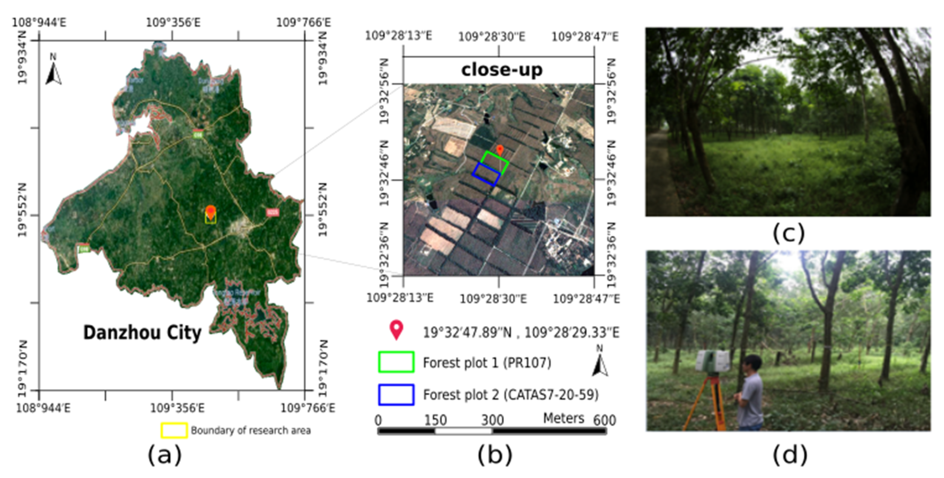
2.1. Study Site and Data Collection

The study area was located in Hainan Dan Zhou (north-western area of Hainan Island, 109°430–109°510E; 19°280–19°380N) within a rubber tree plantation. The topography of the study area is a hilly plateau with an elevation of 188 m above sea level at the centre. The plateau is surrounded by flat lands with elevations of 20–160 m. As China’s largest rubber production base, Hainan Island is continuously increasing the cultivation of rubber trees. The plantation has converted over 5000 ha of cultivated land and tropical rain forest since it was established in 1957. Of these lands, nearly 3000 ha were planted with natural rubber [34]. A wide variety of rubber trees clones was planted on the plantation, and in this study, two typical clones were selected: PR107 and CATAS7-20-59 (Figure 1). Based on prior knowledge, CATAS7-20-59 is more resistant to hurricanes than is PR107, although a quantitative analysis has not been performed. Both rubber trees selected in this study belong to the Chinese Academy of Tropical Agricultural Sciences Proving Ground and are managed identically.
In a previous study of rubber tree property retrieval [6], we proved that rubber trees belonging to the same clone have similar topological skeleton structures and phenotypic characteristics. Therefore, two typical rubber trees of each clone (PR107 and CATAS 7-20-59) were selected as the references for constructing the corresponding tree models. The point clouds of the two typical rubber trees, the canopy and skeleton, were obtained using a Leica C10 TLS system in May 2018. The Leica C10 instrument is a 532-nm phase-based scanner with a 360° × 270° upward field-of-view and a laser rate of 5000 points per second. The instrument setting height was 1.15 m, and the range measurement accuracy was ±1.5 mm at a distance of approximately 3.5 m. The circular laser beam diameter and beam divergence of the scanner exit were 3 mm and 0.22 mrad, respectively, yielding a minimum distance between consecutive beams of approximately 0.4 mm at a distance of 3.5 m from the instrument, with a scanning minimum deflection angle of 0.057°. Each tree plot was recorded using three scans around the target tree and using the “normal scanning” mode. The registration of the three point clouds corresponding to the three scans was carried out by manual adjustment based on a procedure in the software Cyclone (Leica Geosystem, Switzerland).
The structures of the two typical rubber trees represented by the TLS point clouds are illustrated in Figure 2a,b. The ground-based scanned point density values were 117,615 points (pts) m−2 and 88,249 pts m−2 for Rubber Tree 1 (PR107) and Rubber Tree 2 (CATAS7-20-59), respectively. The individual tree height, branch diameter, crown width, single-leaf area and angle between the branches were measured in situ. The tree height was measured using a Vertex IV hypsometer. The branch diameter was measured using a diameter tape. Crown widths were obtained as two values measured along two perpendicular directions from the treetop location. The single-leaf area and the angles between the trunk and branches were measured using an LI-3000C portable area metre and an angle measurement device, respectively.

2.2. Data Preprocessing

First, based on the wood-leaf separation method [33], LiDAR points were separated into branch point clouds ( p i b ) and leaf point clouds ( p i l ). The second step required filtering noise from the TLS point cloud, such as isolated laser points. The filtering noise algorithm [35] was adopted. We used balls with radii of 10 cm and removed all the balls containing less than 5 points. Figure 3 shows the wood-leaf separation results and noise reduction results.

2.3. Branch Skeleton Reconstruction

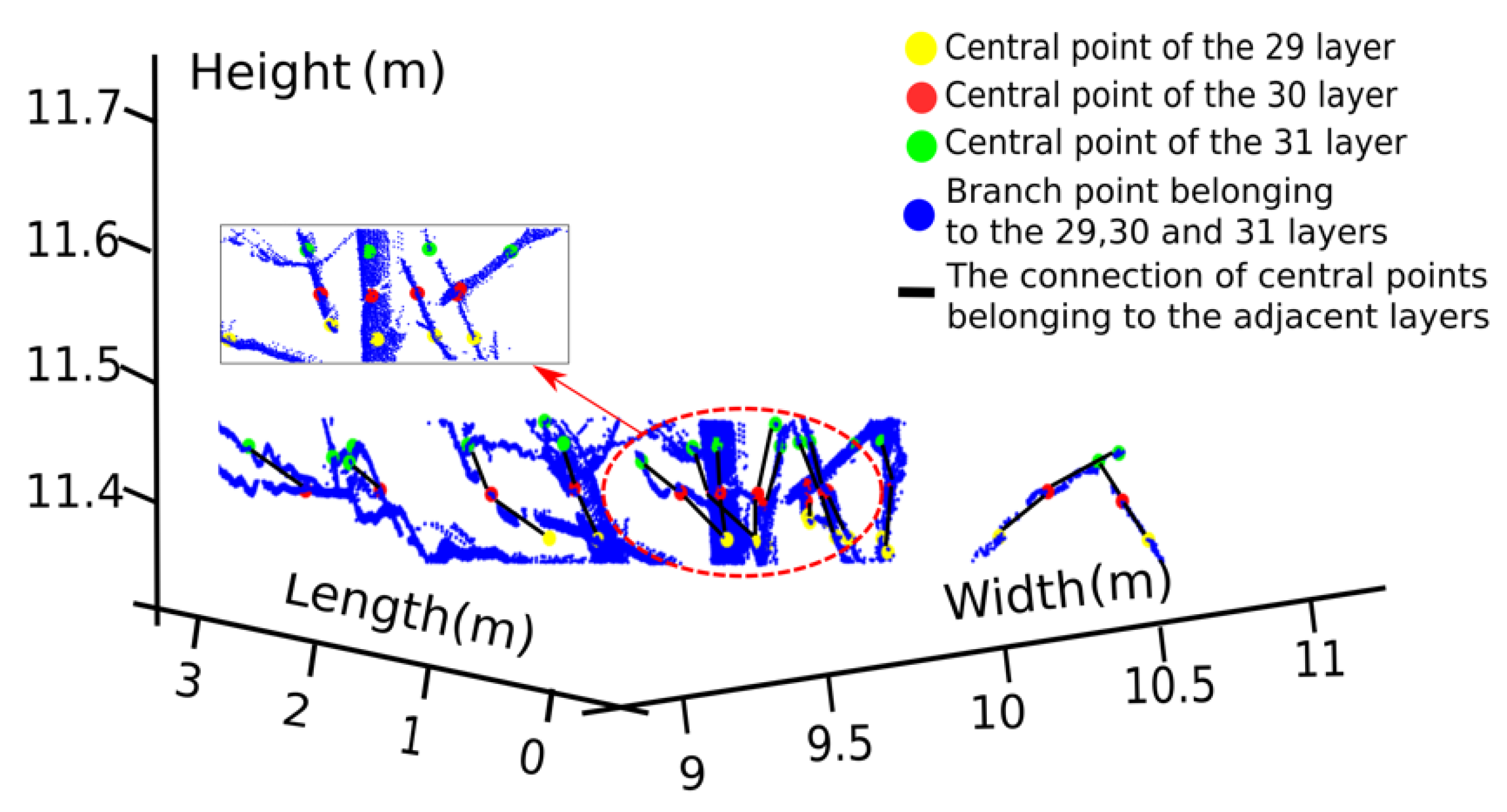
2.3.1. Stratifying Branch Points and Obtaining the Central Points of Each Layer

According to the vertical heights of the individual trees, the branch point cloud is stratified into L e v e l N u m layers from the ground to the highest branch tip, and the number of layers depends on the tree height H t and the height interval Δ h .
L e v e l N u m = H t Δ h
After obtaining the branch point clouds ( p i b ) of every layer, we extract the central point from the branch point clouds ( p i b ) in each layer using the cluster algorithm based on the Euclidean distance [36] with a distance threshold of d i s t 2 . If the distance between each p i b in every layer is less than d i s t 1 , then the set of p i b is identified as one class in this case. Processed by our algorithm, the central point c j l ( c j , x l , c j , y l , c j , z l ) of every layer is extracted, where the jth central points in the lth layer are denoted by c j l . The central point connection between the adjacent layers is based on the minimum Dijkstra distance. As shown in Figure 4, three branch point layers and the central point of each layer are marked with different colours, and the black lines represent the connections between adjacent layers to produce the 3D tree skeleton.

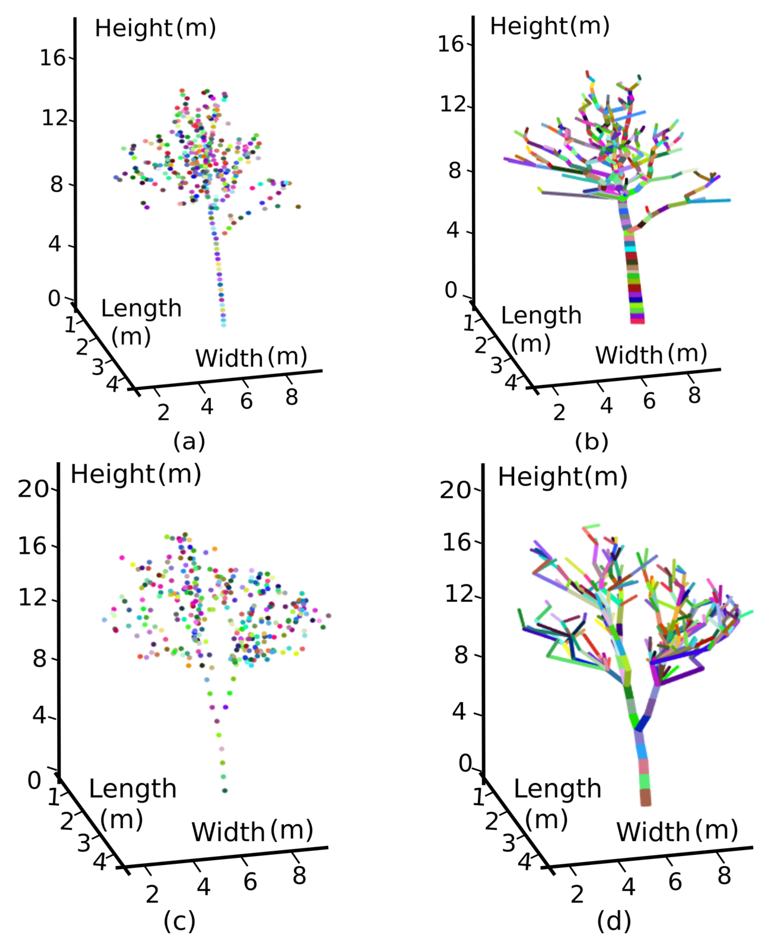
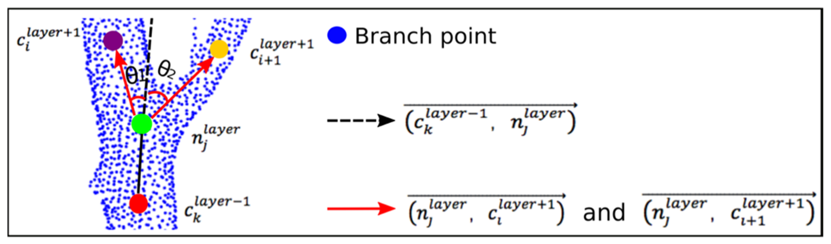
2.3.2. Adopting the Cylinder Model to Form the Tree Skeleton

We define three categories of nodes in bottom-up order to highlight the central points that will be used.
  • Root node: root node c 1 1 is the lowermost central point.
  • Bifurcation node: bifurcation node n j l ( n j l c j l ) has two or more connected child nodes.
  • Edge node: edge node e i l ( e i l c j l ) has no connected child nodes (the nearest central point to c j l is in the upper layer).
In Figure 5, pink points represent the extracted root node c 1 1 , red points represent the extracted edge nodes e j l and green points represent the extracted bifurcation nodes n j l .
Our algorithm begins from root node c 1 1 . According to the k-nearest neighbour and plant growth characteristics, the tree skeleton is transformed into the connection chains from the root node c 1 1 to every edge node e i l . The connection chain between each central point belonging to the adjacent layer is represented by a cylinder D i , j l , l 1 ( c i l , c j l 1 , r ) { l a y e r = 2 , 3 , 4 , , l e v e l n u m } , where r is the radius. According to the plant forest parameters, the diameter of the branch depends on the height; therefore, the lower the layer of the cylinder, the larger is the radius of the cylinder. For each cylinder D i , j l , l 1 ( c i l , c j l 1 , r )   , the radius is based on Dijkstra’s route distance along the connection chain from the central point of the current cylinder to the root node, and this distance is denoted by D i s ( c i l , c 1 1 ) . The radius r of each cylinder can be obtained as follows:
r D i , j l , l 1 = λ × D i s ( c i l , c 1 1 ) 3
where λ is a constant related to the tree clones. As shown in Figure 6, the skeletons of Rubber Tree 1 (PR107) and Rubber Tree 2 (CATAS7-20-59) were reconstructed.

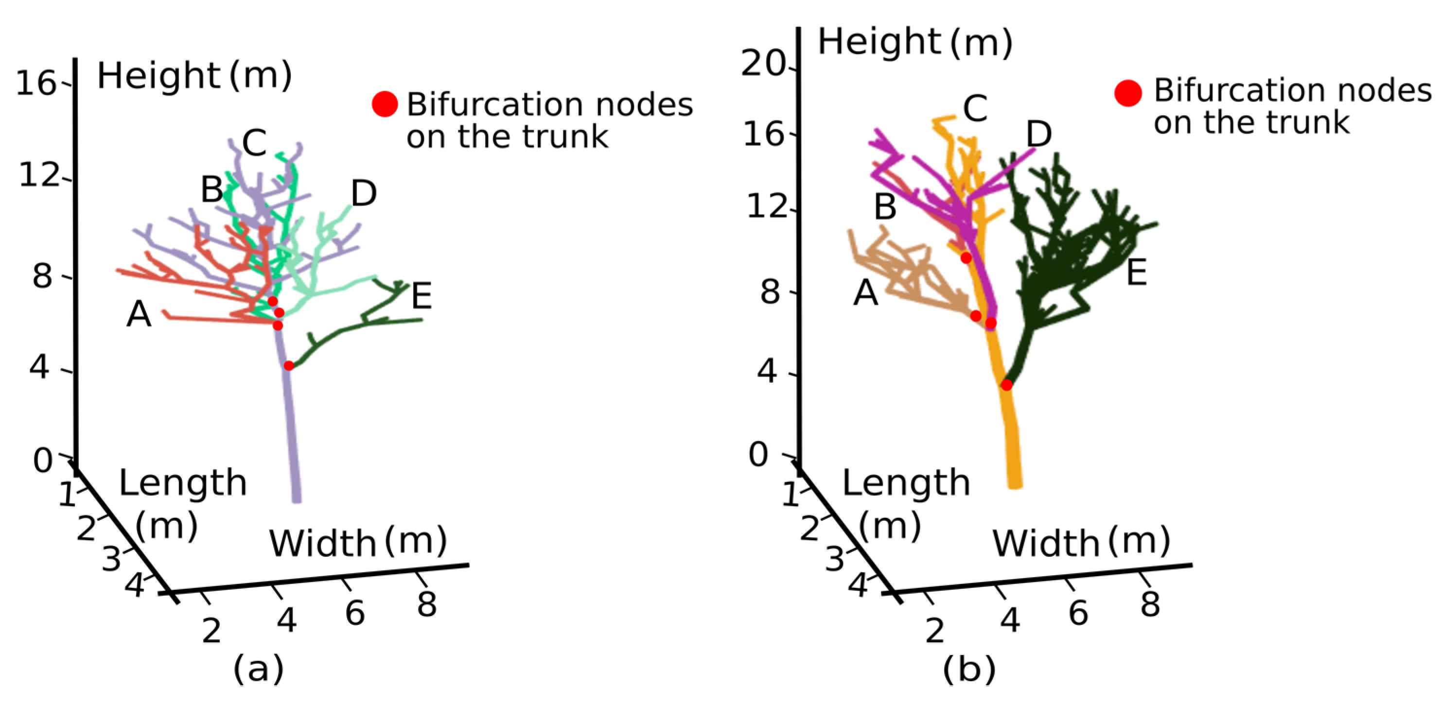
2.3.3. Recognizing the Trunk and First-Order Branches

To more accurately describe the tree skeleton, we divided the tree skeleton into the trunk and many first-order branches. For the rubber tree, the trunk, at least near the base of the tree, is often nearly straight and extends with minimum changes in the growth angle. The trunk is a chain that must start from the root node ( c 1 1 ), and the rest of the chains originating from the trunk will be defined as different first-order branches. Therefore, our algorithm is based on Dijkstra’s algorithm and seeks the connection chain regarding the trunk depending on the rule of minimal change in the growth angle (see Appendix A). For the first-order branches, the connection composed of the central point is searched from the bifurcation nodes on the trunk to the other edge node. In Figure 7, we use different colours to represent our derivation results for the trunk and different first-order branches.

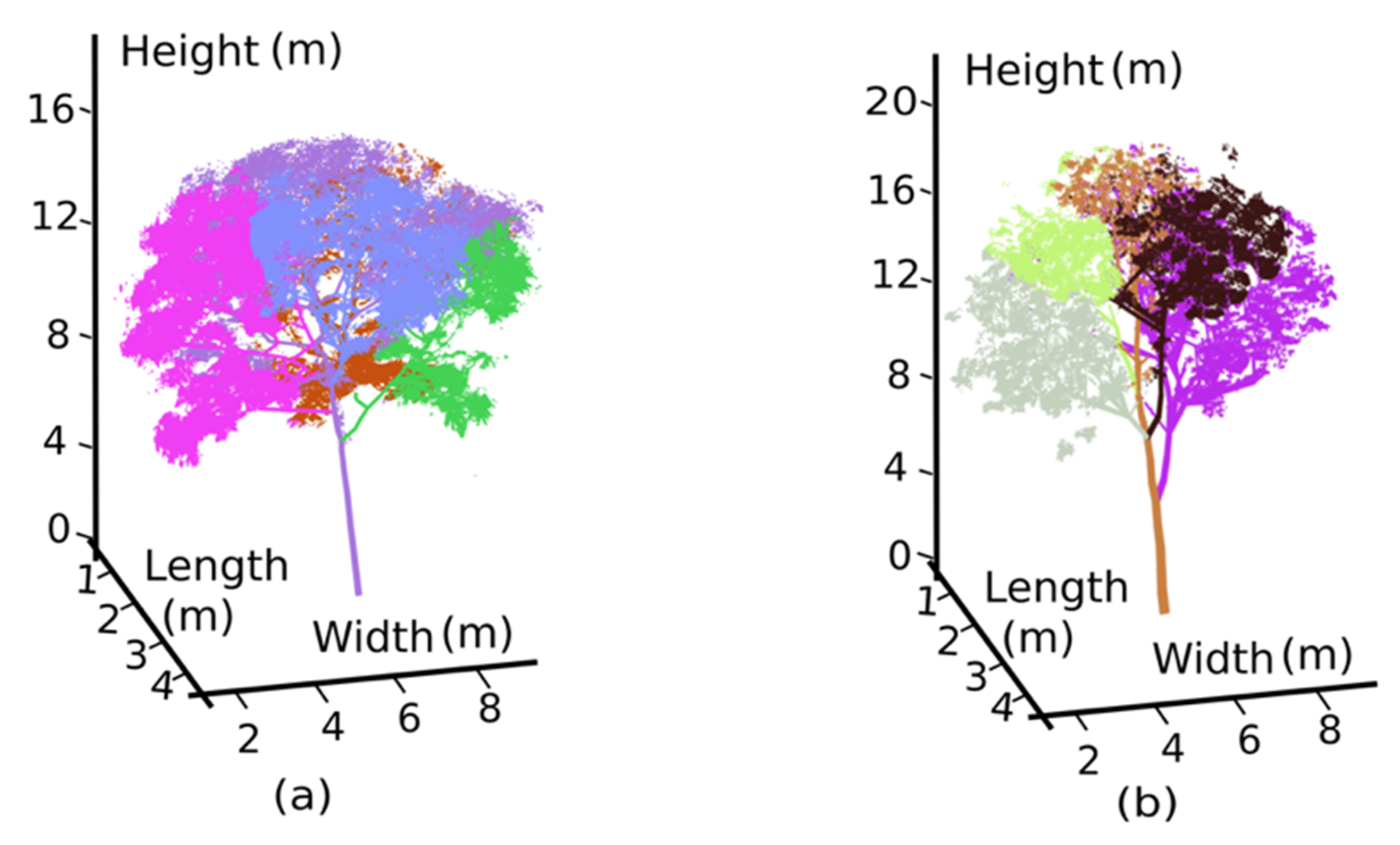
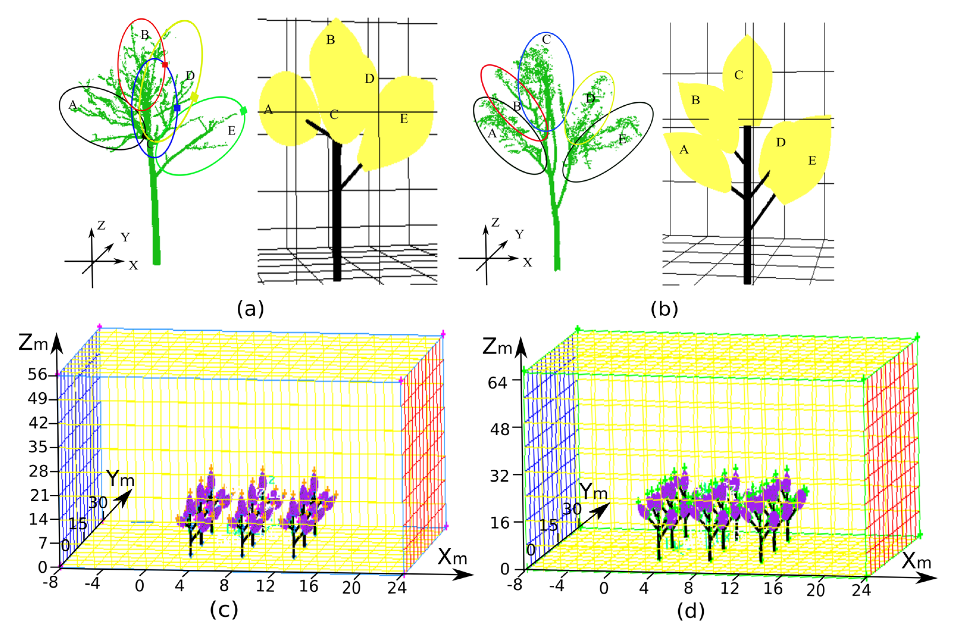
2.3.4. Determining Foliage Clumps based on the Trunk and First-Order Branches

According plant physiological theory, positive pressure resulting from metabolic pumping by the roots draws in water and nutrients from the soil to the leaves via sieve tubes and vessels, and similar hydraulic resistance is observed within vascular tissue via the same branch transport [37], which means that leaves belonging to the same first-order branch have not only a close spatial position and similar illumination but also almost equivalent nutrients and physiological properties [38]. We therefore defined a foliage clump as a leaf collection on the same trunk or first-order branch. The 3D watershed segmentation method [39] was employed to segment the foliage clumps based on the spatial locations of the trunk and first-order branches, and the segmented foliage clumps are represented by different colours (Figure 8).

2.3.5. Retrieving the Foliage Clump Properties

After foliage clump extraction, the parameters of every foliage clump were calculated, including the leaf area index (LAI), crown volume, foliage clump volume, leaf area density and gap fraction. Thus, the 3D reconstruction of the total tree can be simplified into a model consisting of a tree branch skeleton and several foliage clumps.
  • LAI is the ratio of the total leaf area to ground area. First, after the single-leaf extraction and the number of leaves in each foliage clump were obtained using the method described in [29], Delaunay triangulation was adopted to deduce the area of each leaf. We acquired the LAI by computing the ratio of the sum of all leaf areas in each foliage clump to the projected area of each foliage clump.
  • Crown volume and foliage clump volume: A 3D convex hull algorithm [6] was used to deduce the tree crown volume and volume of each foliage clump.
  • Leaf area density: For each foliage clump, the leaf area density was expressed as the ratio of total leaf area to the volume of each foliage clump.
  • Gap fraction: The detailed derivation of the gap fraction of each foliage clump is available in Appendix B.

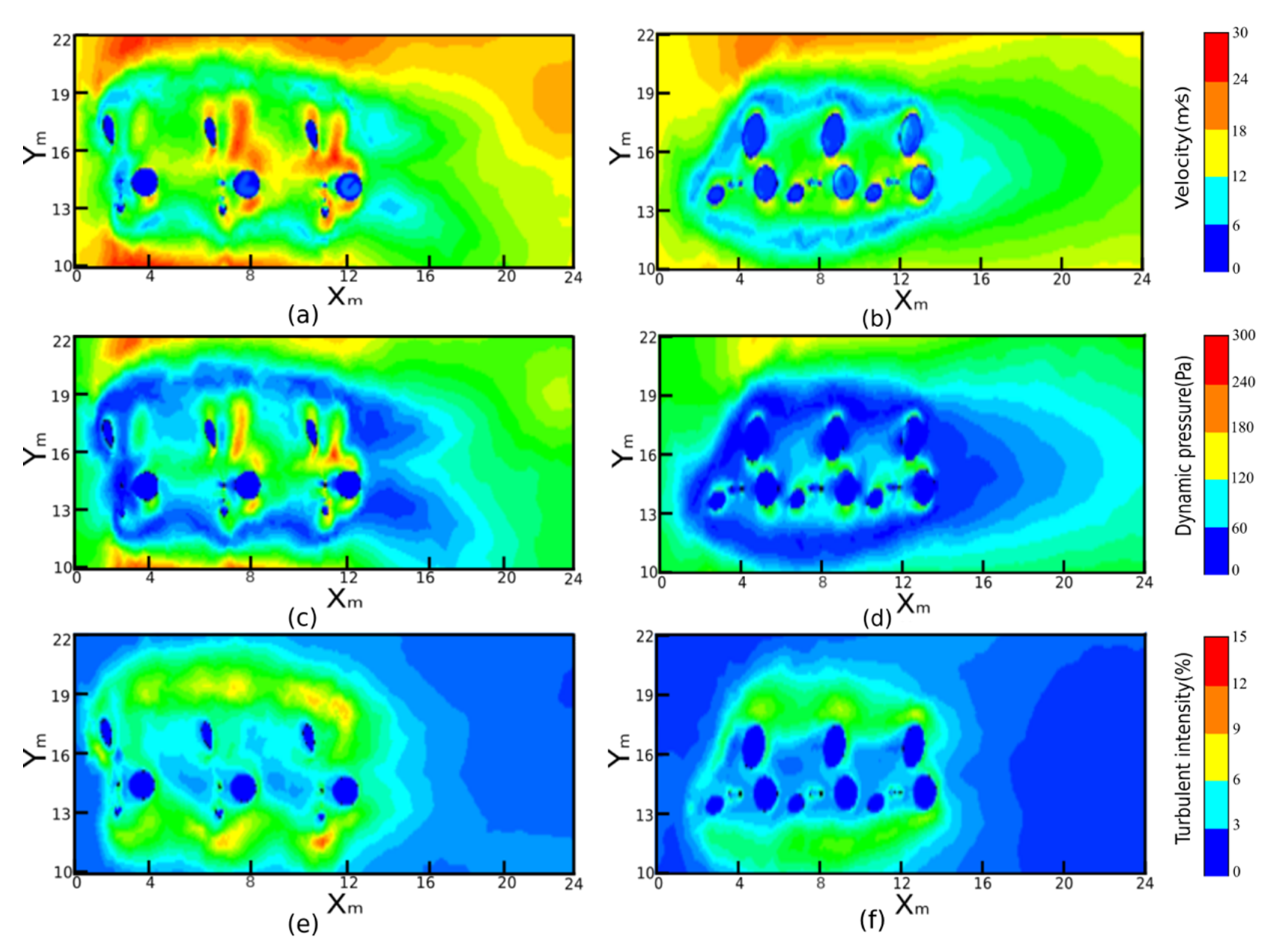
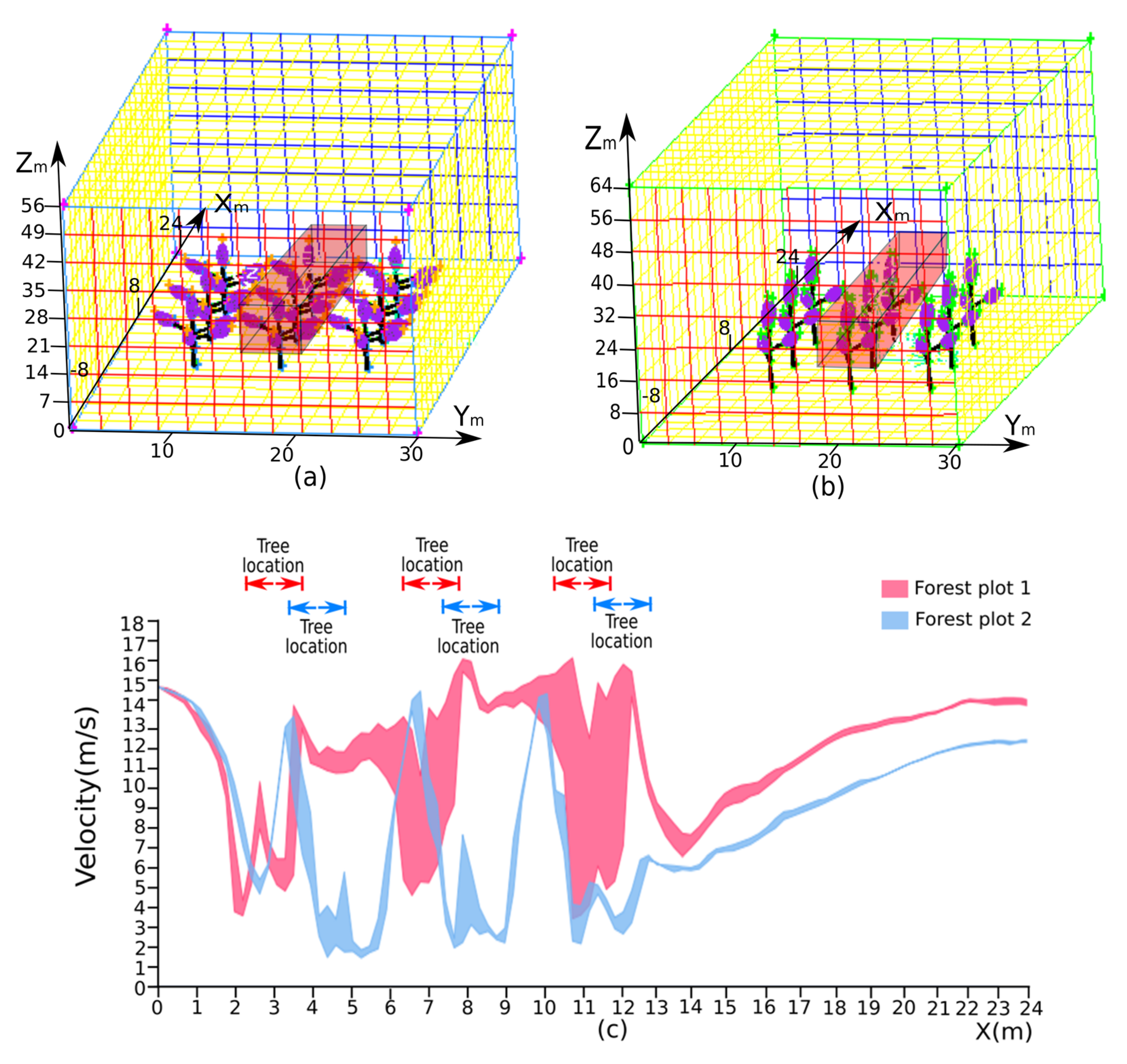
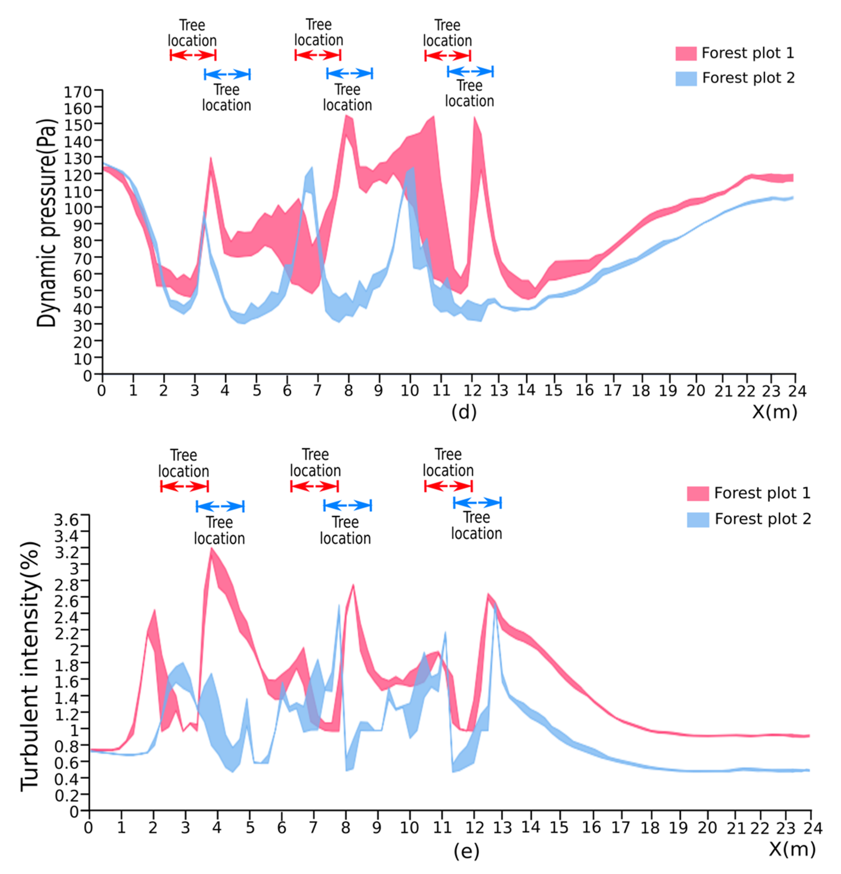
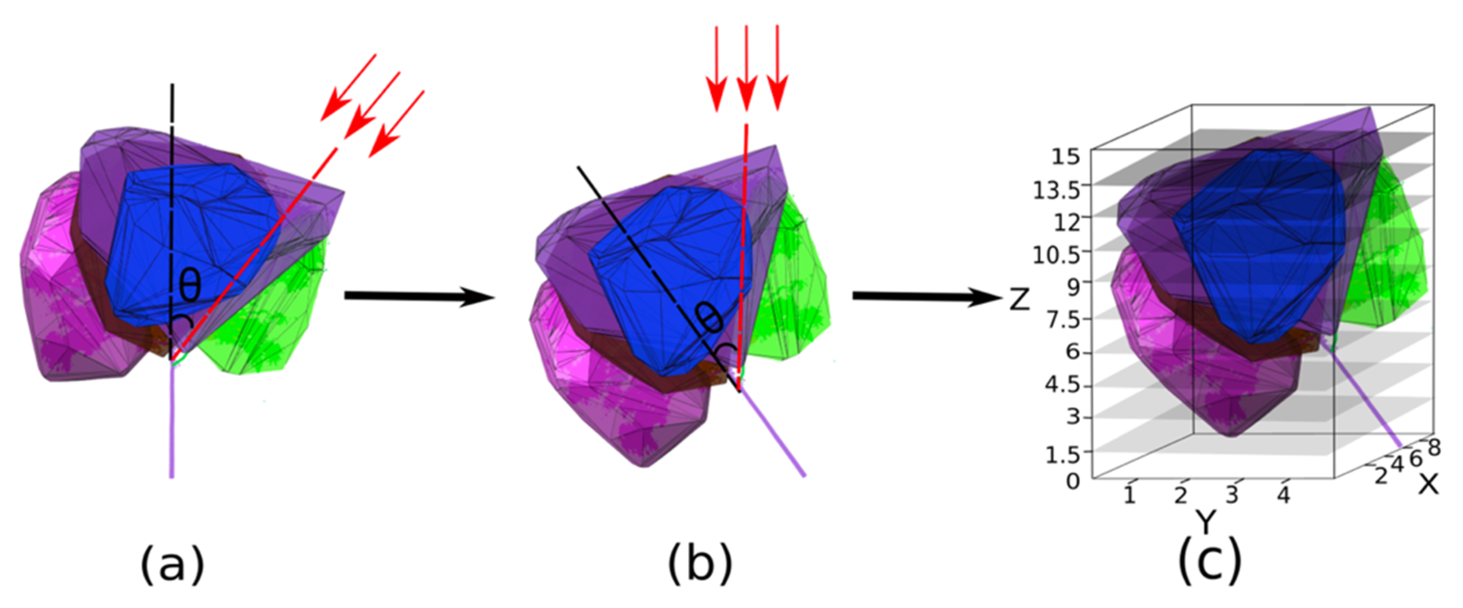
2.3.6. Retrieval of the Wind-Related Parameters in the Rubber Tree Plot

We constructed rubber tree models based on the foliage clump concept proposed in Section 2.3.4. Nine identical rubber tree models of each clone were placed into the plot according to the realistic line and row spacing distances (for PR107 and CATAS7-20-59, the line spacing and row spacing distances were 4 m and 9 m, respectively) to constitute the corresponding forest plot scenarios. After the 3D meshing for the two forest plot scenarios of each clone, the built forest scenario models were brought into the commercial computational fluid dynamics (CFD) software FLUENT (ANSYS Inc., Canonsburg, PA, USA) to simulate a full two-way interaction between the hurricane and forest stands and to calculate the wind-related parameters in the tree plots. The computational model using FLUENT software is based on a standard k-ϵ two equation model [40] (Appendix C affording the full description). The rubber tree plantation in Hainan usually suffers from Level 7 hurricanes with wind speeds of 13.9–17.1 m/s; therefore, we set the wind velocity to 15 m/s, and the results of the specific wind-related parameters in the forest plot, such as the velocity, dynamic pressure and turbulent intensity, are shown in the Results section.

3. Results

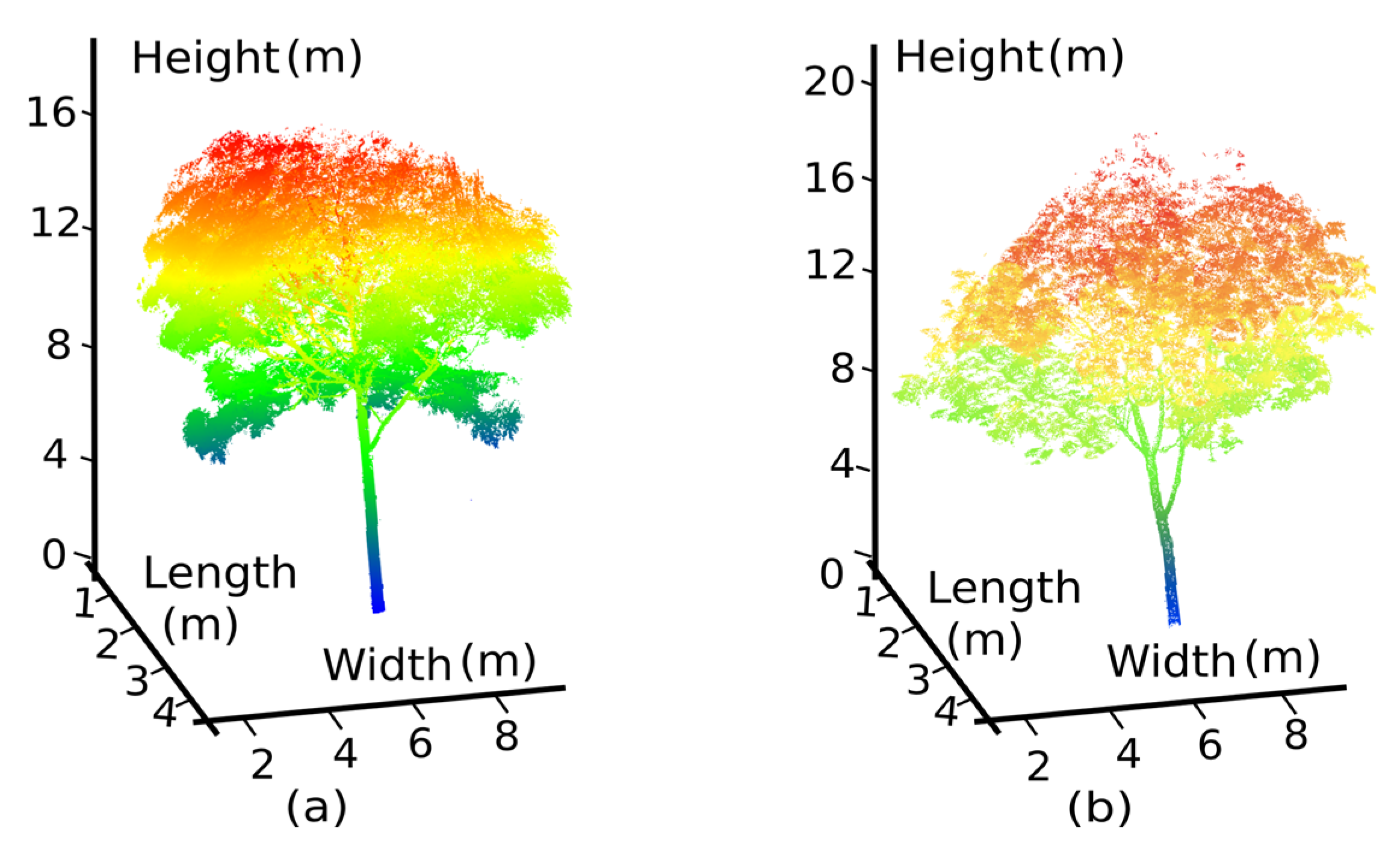
3.1. Properties of the Two Rubber Trees

In our algorithm, for Tree 1 (PR107), the ∆h (in Section 2.3.1.) and λ (in Section 2.3.2.) values were set as 0.05 m and 0.0778, respectively. For Tree 2 (CATAS7-20-59), the ∆h and λ values were set as 0.03 m and 0.0714, respectively.
In this study, some of the forest parameters obtained directly from the point cloud data are listed in Table 1. Other essential parameters were validated by in situ measurements and are listed in Table 2, where A, B, D and E represent first-order branches and C represents the trunk, as shown in Figure 7.
The growth properties of five foliage clumps of Tree 1 (PR107) and Tree 2 (CATAS7-20-59) are shown in Figure 8. We computed the total number of point clouds on each foliage clump, foliage clump volume, projection area, total number of leaves, leaf area, LAI, leaf area density and gap fraction and compared the parameters for the two rubber trees (Table 3).

3.2. Reconstruction of the Forest Plot Model

Nine typical and identical tree models belonging to each clone (PR107 or CATAS 7-20-59) were reconstructed according to the derived foliage clumps and branch attributes using our method, which constitute the corresponding forest plots of two clones. Then, the meshing step for the two forest plots was performed to facilitate the discrete solutions of the aerodynamic formulas (Equations (A9), (A12) and (A13) in Appendix C) for calculation of the aerodynamic parameters in the forest plots, as shown in Figure 9.

3.3. Analysing the Wind-Related Parameters in Forest Plots of Different Clones

According to the hurricane classification criteria in China, hurricanes are divided into six levels in accordance with the maximum wind velocity: Tropical depression (10.8~17.1 m/s); Tropical storm (17.2~24.4 m/s); Severe tropical storm (24.5~32.6 m/s); Typhoon (32.7~41.4 m/s); Severe typhoon (41.5~50.9 m/s); and Super Typhoon (>51.0 m/s). Our paper researched severe tropical storm Mirinae, which landed in Wanning, Hainan, on July 26, 2016. The study retrieved the aerodynamic parameters in the rubber tree forests of the Chinese Academy of Tropical Agricultural Sciences Proving Ground in Danzhou. When Mirinae landed, the maximum wind velocity near the hurricane eye was 25 m/s. It then moved northwestward and arrived in Danzhou at 6 a.m. the next day with the maximum wind velocity near the hurricane eye 18 m/s. Since the rubber tree experimental farm is approximately 15 km away from the hurricane eye, two forest plots composed of rubber trees of clone PR107 and CATAS7-20-59 were placed under the load of a hurricane with a speed of 15 m/s. We studied three trees in the second (middle) row and obtained the velocity, dynamic pressure and turbulent intensity results in the horizontal and vertical profiles, as shown in Figure 10 and Figure 11.
First, by comparing the horizontal section (Z = 7 m) of the velocity distribution for the two forest plots, Figure 10a,b shows that the velocity inside Forest Plot 1 has a larger fluctuation range and a speed of up to 24 m/s in the canopies of the second and third trees (approximately X = 7~8 m and 11~12 m). In contrast, inside Forest Plot 2, the velocity is relatively evenly distributed and less than that of Forest Plot 1. Large speed changes occur on both sides of the rubber trees in rows (Y = 10~12 m and 19~22 m) because the hurricane propagation meets the barrier composed of rubber trees and rushes through the spacing between the trees. Figure 11a,b presents the vertical velocity profiles (Y = 15 m). The maximal values exceed 24 m/s and are mainly located in the windward area above the tree crown of Forest Plot 1.
Second, from Figure 10c,d, for Forest Plot 1 (PR107), the dynamic pressure (i.e., the kinetic energy per unit volume of a fluid particle) value is relatively higher than that of Forest Plot 2 (CATAS7-20-59) and changes drastically inside a single tree, especially in the canopy of the third tree (X = 11~13 m), reaching above 180 Pa. In contrast, in Forest Plot 2, the dynamic pressure tends to be stable and generally less than 120 Pa. Then, we focused on a vertical section of dynamic pressure (Figure 11c,d). A great change in pressure occurs near the windward area of the forest tops in Forest Plot 1 (Z = 16~42 m), and this change is not as marked in Forest Plot 2. Local maxima in the horizontal and vertical profiles of dynamic pressure are both formed in Forest Plot 1 (Figure 10c and Figure 11c), with one on the leeside of the tree and another above the windward side of the crown, and the dynamic pressure in both places exceeds 180 Pa.
Finally, Figure 10e,f shows the turbulent intensity (i.e., the ratio of the standard deviation of the fluctuating wind velocity to the mean wind speed) between the two forest plots. Turbulent intensity is a measure of the degree of pulsation of airflow velocity, and generally divided into three categories according to magnitude: high turbulence (5%–20%), medium turbulence (1%–5%) and low turbulence (less than 1%). The larger the turbulent intensity, the more chaotic the behaviour of the airflow motion. Upon combination with Figure 11e, it is obvious that unstable turbulence (up to 15%) occurs in both sides of Forest Plot 1, which means that the air flows in Forest Plot 1 present a high variation in wind velocity and generate a high wind shear force. Coupled with high LAI and larger crown volumes leading to the increment in the frontal area opposing wind flow and small gaps among the forests, hurricanes in Forest Plot 1 generate strong interactions with vegetative elements and are prone to generate branch breakage and serious defoliation. However, in Forest Plot 2 (Figure 10f and Figure 11f), the turbulent intensity changes are not obvious and are generally lower than 5%, hinting at minor fluctuations of wind velocity existing and air flowing more smoothly. Overall, the influence of inhomogeneities in the aerodynamic parameters of Forest Plot 1 is more pronounced than that of Forest Plot 2, which leads to a greater possibility of wind-induced tree body damage in Forest Plot 1.
We extracted a cuboid region (length x = 0~24 m, width y = 13~18 m and height z = 8~16 m in Forest Plots 1 and 2) to represent the specific wind-related parameter distribution in the middle of the forest canopy, as shown in Figure 12a,b. The range area graphs of velocity, dynamic pressure and turbulent intensity in the cuboids of the two forest plots are shown in Figure 12c,e. Seen from the graph of velocity (Figure 12c), the wind velocity in Plot 1 and Plot 2 tend to decrease when meeting the tree canopy due to the interception of the vegetative elements in the tree canopy. Meanwhile, Figure 12c shows a larger velocity fluctuation in the tree canopies at X = 6~8 m and 10~12 m of Forest Plot 1 than that in the Forest Plot 2. Figure 12d shows the distribution of dynamic pressure in the cuboid regions of the forest plots, and it can be generally seen that the trend of the dynamic pressure distribution is the same as that of the velocity distribution. The explanation of this case is the square of the velocity proportional to the dynamic pressure based on Bernoulli’s equation [41]. Figure 12e shows the distribution of turbulent intensity in each cuboid region of the two forest plots. The turbulent intensity represents the intensity of wind velocity fluctuation [42]. A low gap fraction of the typical trees in Forest Plot 1 induced by higher leaf area density results in a local strong wind current entering the tree canopy, which causes the velocity to fluctuate greatly in the red area of the forest canopy at X = 3~4 m, 7~8 m and 12~13 m. Overall, the velocity, dynamic pressure and turbulent intensity of Forest Plot 1 are generally higher than those of Forest Plot 2, resulting in higher vulnerability to hurricane damage for Forest Plot 1 than for Forest Plot 2.

4. Discussion

In this study, we adopted a balance between the forest scale and individual tree scale, used the concept of foliage clumps to facilitate rubber tree modelling and retained the original morphological characteristics of rubber trees. The simplified model developed in this paper could represent the first step towards a new generation of medium-view models for simulating broad-leaf trees. Simplification into foliage clumps decreases the number of simulated leaves for which calculations must be performed and retains the local phenotypic characteristics of the rubber tree crown. Multi-disciplinary approaches from aerodynamics [43], forestry and computer graphics were combined to reconstruct various forest plot scenarios and to simulate the wind fields in different rubber tree plots to quantitatively analyse the distribution of the wind-related parameters. The method used in this paper is flexible and can be extended to any broad-leaved tree species because the branching habits of broad-leaved trees and their phenotypic characteristics are similar. Through computer simulation techniques, spatial planning, wind speeds and the phenotypic characteristics of tree species (such as the gap fraction, LAI, canopy volume, etc.) can be adjusted to quantitatively investigate the aerodynamic parameters of different stands under windy conditions. Moreover, comparing the damage risk of rubber tree plots in this research provides a better understanding of the differences in damage patterns among the two rubber tree clones and provides guidelines for suitable silvicultural management practices.
The simulation results are difficult to verify empirically. Experimental manipulations of wind at the scale of forest stands are impossible. Obtaining measurements during a hurricane is dangerous, and it is difficult to protect sensitive equipment from wind and rain damage during extreme weather. Our approach to stand reconstruction is generally applicable to broad-leaved trees but will not transfer as readily to conifers, which remain poorly covered by existing wind risk models. This is due to several limitations. Terrestrial laser scanning is an inappropriate tool with which to detect conifer needles, as they are generally smaller than the characteristic laser spot size. It is difficult to represent needles using point clouds, and the relationship between needles and the mechanical load of wind is hard to predict.
Our simulation results reveal a contrast between Forest Plot 1 (PR107) and Forest Plot 2 (CATAS7-20-59). Trees in Forest Plot 1 become more vulnerable to damage than do those in Forest Plot 2 because of the stronger velocity, dynamic pressure and turbulent intensity, particularly between the trunk and first-order branches. The analytical conclusion from our algorithm is consistent with the experience of rubber tree growers. Tree characteristics, such as gap fraction and shape, may be significant predictors of wind damage. Rubber trees of clone PR107 present a higher LAI and lower gap fraction than do rubber trees of clone CATAS 7-20-59, which means that the leaves of the rubber trees of clone PR107 are denser and cause considerable wind drag on the tree crown. Previous studies of wind damage in forests have suggested that trees with large, dense crowns produce large wind drag, resulting in tree lodging [44,45]. Moreover, the rubber trees of clone CATAS 7-20-59, which present a small angle between the trunk and the first-order branches to form an ascending vase shape for the tree crown, have a considerably more stable tree crown structure than do the rubber trees of clone PR107, with a spread-out tree crown under the impact of wind. The effect of tree shapes on wind firmness is also well documented [44,45], and tree architecture itself can alter the magnitude and the spatial distribution of wind loading [46].

5. Conclusions

Based on our findings obtained from the simulation program, the following strategies are suggested to reduce the risk of windthrow:
  • Trees with large or dense crowns are more vulnerable to windthrow than are trees with smaller open crowns. Crown modification techniques, such as pruning and topping to reduce the effective crown size and density, can considerably reduce the risk of windthrow. Where possible, creating gaps that are too large and exposing individual branches or foliage clumps through these types of cuts should be avoided.
  • A wide variety of rubber tree clones is planted in the coastal areas of China. The choice of rubber tree clones should take into account the probability of wind damage. Before extensively promoting a new clone of rubber trees, our method can be used to analyse the forest parameters, determine their aerodynamic parameters under windy conditions and measure the resistance capability of tree clones.
  • Quantification of wind damage under different forest cultivation practices (e.g., adjusting the spatial distance between trees or changing the arrangement of trees) in the forest can be explored using our method to analyse to identify suitable silvicultural management strategies for different rubber tree clones.
Such management strategies will promote wind-resistant tree characteristics and help mitigate the risk of tree failures and subsequent economic damage.

Author Contributions

Conceptualization, T.Y.; data curation, F.A. and B.C.; formal analysis, Z.H.; funding acquisition, T.Y.; methodology, X.H.; project administration, T.Y.; software, Z.H. and X.H.; supervision, T.Y.; validation, F.A. and B.C.; visualization, Z.H. and T.Y.; writing—original draft, Z.H. and X.H.; writing—review and editing, M.E., J.F., L.C., Z.Z. and T.Y. All authors have read and agreed to the published version of the manuscript.

Funding

This work was supported by the National Natural Science Foundation of China (grant numbers 31770591, 41701510), the Central Public-interest Scientific Institution Basal Research Fund for the Chinese Academy of Tropical Agricultural Sciences (grant numbers 1630022020002) and the Priority Academic Program Development of Jiangsu Higher Education Institutions (PAPD).

Acknowledgments

The authors gratefully acknowledge the foresters in the Chinese Academy of Tropical Agricultural Sciences Proving Ground for their assistance with data collection and sharing their rich knowledge and working experience.

Conflicts of Interest

The authors declare no conflicts of interest.

Appendix A. Rule of Minimal Change in the Growth Angle

To determine the trunk chain, first, beginning from the root node ( c 1 1 ), the node connected to the root node ( c 1 1 ) is stored in a queue until meeting a bifurcation node ( n j l a y e r ). Secondly, as suggested by Figure A1, to implement the trunk chain determination, our algorithm presents a minimal change judgement method based on an angle value comparison. For bifurcation nodes ( n j l a y e r ) on the trunk chain with multiple central points ( c i l a y e r + 1 and c i + 1 l a y e r + 1 ) in the upper layer, we define the included angle ( ( c k l a y e r 1 , n j l a y e r ) , ( n j l a y e r , c i l a y e r + 1 ) ) as θ 1 . Similarly, we define the second included angle ( ( c k l a y e r 1 , n j l a y e r ) , ( n j l a y e r , c i + 1 l a y e r + 1 ) ) as θ 2 . Thirdly, the chain that belongs to the trunk is determined by comparing θ 1 and θ 2 . We choose the chain with the minimum change in the direction angle as the trunk chain, and the angle comparison equation is as follows:
{ i f   θ 1 < θ 2 , ( c k l a y e r 1 , n j l a y e r , c i l a y e r + 1 )   c o n s t i t u t e s   t r u n k i f   θ 1 θ 2 , ( c k l a y e r 1 , n j l a y e r , c i + 1 l a y e r + 1 )   c o n s t i t u t e s   t r u n k k = 1 , 2 , 3 ; i = 1 , 2 , 3
Finally, when the edge node is determined, the central point belonging to the chain that begins from the root node is classified as the trunk.
Figure A1. Our algorithm for performing trunk chain extraction using the rule of minimal change in the growth angle. If bifurcation nodes n j l a y e r occur in the trunk chain, we compare the included angle between ( c k l a y e r 1 , n j l a y e r ) and ( n j l a y e r , c i l a y e r + 1 ) or ( n j l a y e r , c i + 1 l a y e r + 1 ) and take the trunk chain composed of the central points ( c k l a y e r 1 , n j l a y e r , c i l a y e r + 1 )   , depending on the rule of minimal angle change, as the trunk.
Remotesensing 12 01318 g0a1

Appendix B. Derivation of the Gap Fraction

Each foliage clump is a collection of leaves and records the partial features of the whole tree crown. According to theoretical principles [47,48], by assuming that the inside of each foliage clump is a turbid medium, we have the following equation:
a z , θ = 1 S z , θ S z , θ e x p ( G ( θ ) L D s ( x , y , z , θ ) ) d x d y
where a z , θ is the gap fraction of each foliage clump along the θ direction at a height above z ; S z , θ is the projection area of the foliage clump at the inclination angle θ at any height z ; ( x , y , z ) is the scanned point; G ( θ ) is the extinction coefficient defined as the projection of the unit foliage area on the plane perpendicular to the inclination angle θ ; and L D is the leaf area density. s ( x , y , z , θ ) is the optical path through which the photon reaches a point in the direction θ , but s ( x , y , z , θ ) cannot be explicitly determined and results in the lack of a calculated value for a z , θ . In this paper, we apply Equation (A3) as an approximate transform to retrieve a z , θ :
a z , θ e x p ( G ( θ ) L D s ˜ ( z , θ ) )
s ˜ ( z , θ ) is the approximation of s ( x , y , z , θ ) , and we have the following equation:
s ˜ ( z , θ ) = V ( z ) / ( S z , θ c o s θ )
where V ( z ) is the volume of the foliage clumps above height z .
G ( θ ) is calculated as follows:
First, taking Tree 1 (PR107) as an example, the point cloud data of the tree are first rotated into a necessary position with an inclination angle θ (Figure A2b). Then, the voxelization procedure is applied to the rotated tree. By defining the width w , length l and height h for each voxel, the tree domain is divided into m × n × p voxels, where m = ( x m a x x m i n ) / w , n = ( y m a x y m i n ) / l , and p = ( z m a x z m i n ) / h . After the voxelization process of the Rubber Tree 1 (PR107) domain, each row or column layer is regarded as a plane that extracts a part of the dataset, which is defined as a slice plane.
Secondly, the mean projection coefficient at the lth layer slice plane G l ( θ ) for the incident radiation with an inclination angle θ can be calculated by integrating the azimuth angle φ over the range [ 0 ,   2 π ] as follows:
G l ( θ ) = 0 2 π G l ( r ) d φ
where r ( θ , φ ) is the incoming direct solar beams formed by the inclination angle θ and the azimuth angle φ .
Thirdly, this step involves calculating the projection coefficient for a given direction. We first consider the incoming direct solar beams with a direction r ( θ , φ ) and take a slice plane perpendicular to the beam. Based on the method described in [49], the projection coefficient can be obtained by computing the ratio of the real foliage area A ξ to the projected foliage area A P , ξ , where ξ is the ξ th nonempty voxel in the lth slice layer. We construct a 3D convex hull based on the points in the nonempty voxel to represent the projected foliage area A P , ξ , and one-half of the total surface area of this 3D convex hull is used to represent the real foliage area A ξ . By summarizing the projection coefficients for a single slice plane normal to the direction of incident radiation, we have the following equation:
G l ( r ) = 1 S ξ = 1 S A P , ξ / A ξ
where S is the total number of nonempty voxels in the lth slice plane.
The mean projection coefficient in the lth-layer slice plane G l ( θ ) can be obtained from Equation (A5). The total mean projection coefficient under the canopy for the incoming direct solar beams with direction r ( θ , φ ) equals the following equation:
G ( θ ) = l = 1 p G l ( θ ) p
where p is the total number of slice planes. By combining Equations (A7) and (A3), we have the following equation:
a z , θ e x p ( l = 1 M G l ( θ ) p L D V ( z ) / ( S z , θ c o s θ ) )
The leaf area density L D is calculated as shown above, and V ( z ) is calculated using a 3D convex hull. S z , θ is calculated as the projection area of Figure A2c with an incident angle θ . We obtain the formula that can directly provide the gap fraction a z , θ of each foliage clump.
Figure A2. Schematic diagrams illustrating the extinction coefficient calculation. (a) Three-dimensional convex hull construction based on the point cloud data of each foliage clump in Rubber Tree 1 (PR107). (b) Tree rotated counter-clockwise into the required relative position, and (c) nine horizontal slicing planes for Rubber Tree 1 (PR107) with a bounding box for the convenient extinction coefficient inversion computation.
Remotesensing 12 01318 g0a2

Appendix C. Standard k-ϵ Two Equation Model

Appendix C.1. Momentum Model

According to the momentum conservation law and Navier–Stokes equations, the momentum model is described by Equation (A9).
ρ u j u i x j = p x i + x j μ t ( u x j + u j x i ) ρ u i u j ¯ x j + S i
Here, ρ = 1.293 kg/m³ and represents the density of a fluid; μ t (in kg/m) is the dynamic viscosity described by Equation (A16); p is the pressure of the wind; i and j represent any two directions of x, y and z in a three-dimensional coordinate system; x i and x j are the coordinate components in the i-direction and j-direction, respectively; u i (in m/s) is the wind speed in the i-direction; u j (in m/s) is the wind speed in the j-direction; and S i is the source term in the i-direction described by Equation (A10):
S i = C d 1 2 ρ | u j | u j
where C d is the drag coefficient of the tree crown, and it is described with the LAI by Equation (A11):
C d = 0.549 0.589 1 + e x p ( ( L A I 0.393 ) / 0.146 )
where the LAI can be obtained in Section 2.3.5.

Appendix C.2. k ϵ Model

The k ϵ model overcomes the problem with flow close to the surface elements due to a singularity in the governing equations, and the k ϵ model is described using the turbulent kinetic energy k and dissipation rate ϵ by Equations (A12) and (A13), respectively. The turbulent kinetic energy k and the dissipation rate ϵ in a fully developed neutral atmospheric boundary layer are defined by Equations (A14) and (A15), respectively.
ρ D k D t = X j ( μ t σ k k X j ) + μ t ( u i x j + u j x i ) u i x j ρ ε
ρ D ε D t = X j ( μ t σ ε ε X j ) + C ε 1 μ t ε k ( u i x j + u j x i ) u i x j ρ C ε 2 ε 2 k
k = 1 2 u i 2 ¯
ε = μ t ρ ( u i x j ) 2 ¯
μ t = ρ C μ k 2 ε
As shown in Table A1, C μ , C ε 1 ,   C ε 2 , σ k and σ ε are momentum and turbulence equation constants used for simulating the forest canopy to retrieve some wind parameters. By combining Equations (A9), (A12) and (A13), the velocity, dynamic pressure and turbulent intensity can be deduced.
Table A1. Momentum and turbulence equation constants used for simulating the forest canopy
C μ C ε 1 Cε2 σ k σ ε
0.091.421.921.01.3

References

  1. Li, L.; Kareem, A.; Xiao, Y.; Song, L.; Zhou, C. A comparative study of field measurements of the turbulence characteristics of typhoon and hurricane winds. J. Wind Eng. Ind. Aerodyn. 2015, 140, 49–66. [Google Scholar] [CrossRef]
  2. Dupont, S.; Pivato, D.; Brunet, Y. Wind damage propagation in forests. Agric. For. Meteorol. 2015, 214, 243–251. [Google Scholar] [CrossRef]
  3. Change, C. The Physical Science Basis; Intergovernmental Panel on Climate Change: Geneva, Switzerland, 2013. [Google Scholar]
  4. Xia, Z.; Liu, K.; Zhang, S.; Yu, W.; Zou, M.; He, L.; Wang, W. An ultra-high density map allowed for mapping QTL and candidate genes controlling dry latex yield in rubber tree. Ind. Crops Prod. 2018, 120, 351–356. [Google Scholar] [CrossRef]
  5. Suchat, S.; Theanjumpol, P.; Karrila, S. Rapid moisture determination for cup lump natural rubber by near infrared spectroscopy. Ind. Crops Prod. 2015, 76, 772–780. [Google Scholar] [CrossRef]
  6. Yun, T.; Jiang, K.; Hou, H.; An, F.; Chen, B.; Jiang, A.; Li, W.; Xue, L. Rubber Tree Crown Segmentation and Property Retrieval using Ground-Based Mobile LiDAR after Natural Disturbances. Remote Sens. 2019, 11, 903. [Google Scholar] [CrossRef] [Green Version]
  7. Schelhaas, M.-J.; Hengeveld, G.; Moriondo, M.; Reinds, G.J.; Kundzewicz, Z.W.; Ter Maat, H.; Bindi, M. Assessing risk and adaptation options to fires and windstorms in European forestry. Mitig. Adapt. Strateg. Glob. Chang. 2010, 15, 681–701. [Google Scholar] [CrossRef]
  8. Zhu, J.; Li, X.; Liu, Z.; Cao, W.; Gonda, Y.; Matsuzaki, T. Factors affecting the snow and wind induced damage of a montane secondary forest in northeastern China. Silva. Fenn. 2006, 40, 37. [Google Scholar] [CrossRef] [Green Version]
  9. Gardiner, B.; Berry, P.; Moulia, B. Wind impacts on plant growth, mechanics and damage. Plant Sci. 2016, 245, 94–118. [Google Scholar] [CrossRef]
  10. Hayashi, M.; Saigusa, N.; Oguma, H.; Yamagata, Y.; Takao, G. Quantitative assessment of the impact of typhoon disturbance on a Japanese forest using satellite laser altimetry. Remote Sens. Environ. 2015, 156, 216–225. [Google Scholar] [CrossRef]
  11. Villamayor, B.M.R.; Rollon, R.N.; Samson, M.S.; Albano, G.M.G.; Primavera, J.H. Impact of Haiyan on Philippine mangroves: Implications to the fate of the widespread monospecific Rhizophora plantations against strong typhoons. Ocean. Coast. Manag. 2016, 132, 1–14. [Google Scholar] [CrossRef]
  12. Dolan, K.A.; Hurtt, G.C.; Chambers, J.Q.; Dubayah, R.O.; Frolking, S.; Masek, J.G. Using ICESat’s Geoscience Laser Altimeter System (GLAS) to assess large-scale forest disturbance caused by hurricane Katrina. Remote Sens. Environ. 2011, 115, 86–96. [Google Scholar] [CrossRef]
  13. Peltola, H.; Ikonen, V.-P.; Gregow, H.; Strandman, H.; Kilpeläinen, A.; Venäläinen, A.; Kellomäki, S. Impacts of climate change on timber production and regional risks of wind-induced damage to forests in Finland. For. Ecol. Manag. 2010, 260, 833–845. [Google Scholar] [CrossRef]
  14. Rich, R.L.; Frelich, L.; Reich, P.B.; Bauer, M.E. Detecting wind disturbance severity and canopy heterogeneity in boreal forest by coupling high-spatial resolution satellite imagery and field data. Remote Sens. Environ. 2010, 114, 299–308. [Google Scholar] [CrossRef]
  15. Lagergren, F.; Jönsson, A.M.; Blennow, K.; Smith, B. Implementing storm damage in a dynamic vegetation model for regional applications in Sweden. Ecol. Modell. 2012, 247, 71–82. [Google Scholar] [CrossRef] [Green Version]
  16. Pivato, D.; Dupont, S.; Brunet, Y. A simple tree swaying model for forest motion in windstorm conditions. Trees 2014, 28, 281–293. [Google Scholar] [CrossRef]
  17. Schelhaas, M.J. The wind stability of different silvicultural systems for Douglas-fir in the Netherlands: A model-based approach. Forestry 2008, 81, 399–414. [Google Scholar] [CrossRef] [Green Version]
  18. Sylvain, D.; Veli-Pekka, I.; Hannu, V.; Peltola, H. Predicting tree damage in fragmented landscapes using a wind risk model coupled with an airflow model. Can. J. For. Res. 2015, 45, 150409143413008. [Google Scholar]
  19. Locatelli, T.; Tarantola, S.; Gardiner, B.; Patenaude, G. Variance-based sensitivity analysis of a wind risk model-Model behaviour and lessons for forest modelling. Environ. Model. Softw. 2017, 87, 84–109. [Google Scholar] [CrossRef] [Green Version]
  20. Gardiner, B.; Peltola, H.; Kellomäki, S. Comparison of two models for predicting the critical wind speeds required to damage coniferous trees. Ecol. Modell. 2000, 129, 1–23. [Google Scholar] [CrossRef]
  21. Blennow, K.; Andersson, M.; Sallnäs, O.; Olofsson, E. Climate change and the probability of wind damage in two Swedish forests. For. Ecol. Manag. 2010, 259, 818–830. [Google Scholar] [CrossRef]
  22. Watt, M.S.; Moore, J.R.; McKinlay, B. The influence of wind on branch characteristics of Pinus radiata. Trees 2005, 19, 58–65. [Google Scholar] [CrossRef]
  23. James, K.R.; Dahle, G.A.; Grabosky, J.; Kane, B.; Detter, A. Tree biomechanics literature review: Dynamics. Arboric. Urban For. 2014, 40, 1–15. [Google Scholar]
  24. Chiba, Y. Modelling stem breakage caused by typhoons in plantation Cryptomeria japonica forests. For. Ecol. Manag. 2000, 135, 123–131. [Google Scholar] [CrossRef]
  25. Tadrist, L.; Saudreau, M.; De Langre, E. Wind and gravity mechanical effects on leaf inclination angles. J. Theor. Biol. 2014, 341, 9–16. [Google Scholar] [CrossRef] [PubMed]
  26. Zhu, Y.; Shao, C. The steady and vibrating statuses of tulip tree leaves in wind. Theor. Appl. Mech. Lett. 2017, 7, 30–34. [Google Scholar] [CrossRef]
  27. Yun, T.; Cao, L.; An, F.; Chen, B.; Xue, L.; Li, W.; Pincebourde, S.; Smith, M.J.; Eichhorn, M.P. Simulation of multi-platform LiDAR for assessing total leaf area in tree crowns. Agric. For. Meteorol. 2019, 276, 107610. [Google Scholar] [CrossRef]
  28. Sheng, Q.; Zhang, Y.; Zhu, Z.; Li, W.; Xu, J.; Tan, R. An experimental study to quantify road greenbelts and their association with PM2.5 concentration along city main roads in Nanjing, China. Sci. Total Environ. 2019, 667, 710–717. [Google Scholar] [CrossRef]
  29. Xu, Q.; Cao, L.; Xue, L.; Chen, B.; An, F.; Yun, T. Extraction of Leaf Biophysical Attributes Based on a Computer Graphic-based Algorithm Using Terrestrial Laser Scanning Data. Remote Sens. 2019, 11, 15. [Google Scholar] [CrossRef] [Green Version]
  30. Sun, Y.; Liang, X.; Liang, Z.; Welham, C.; Li, W. Deriving Merchantable Volume in Poplar through a Localized Tapering Function from Non-Destructive Terrestrial Laser Scanning. Forests 2016, 7, 87. [Google Scholar] [CrossRef]
  31. Hu, C.; Pan, Z.; Zhong, T. Leaf and wood separation of poplar seedlings combining locally convex connected patches and K-means++ clustering from terrestrial laser scanning data. J. Appl. Remote Sens. 2020, 14, 1. [Google Scholar] [CrossRef]
  32. Hu, C.; Pan, Z.; Li, P. A 3D Point Cloud Filtering Method for Leaves Based on Manifold Distance and Normal Estimation. Remote Sens. 2019, 11, 198. [Google Scholar] [CrossRef] [Green Version]
  33. Xu, S.; Xu, S.; Ye, N.; Zhu, F. Automatic extraction of street trees’ nonphotosynthetic components from MLS data. Int. J. Appl. Earth Obs. Geoinf. 2018, 69, 64–77. [Google Scholar] [CrossRef]
  34. Chen, B.; Cao, J.; Wang, J.; Wu, Z.; Tao, Z.; Chen, J.; Yang, C.; Xie, G. Estimation of rubber stand age in typhoon and chilling injury afflicted area with Landsat TM data: A case study in Hainan Island, China. For. Ecol. Manag. 2012, 274, 222–230. [Google Scholar] [CrossRef]
  35. Xu, S.; Wang, R. Power Line Extraction from Mobile LiDAR Point Clouds. IEEE J. Sel. Top. Appl. Earth Obs. Remote Sens. 2019, 12, 734–743. [Google Scholar] [CrossRef]
  36. Yang, H.; Yang, X.; Zhang, F.; Ye, Q. Robust Plane Clustering Based on L1-Norm Minimization. IEEE Access 2020, 8, 29489–29500. [Google Scholar] [CrossRef]
  37. Savage, J.A.; Beecher, S.D.; Clerx, L.; Gersony, J.T.; Knoblauch, J.; Losada, J.M.; Jensen, K.H.; Knoblauch, M.; Holbrook, N.M. Maintenance of carbohydrate transport in tall trees. Nat. Plants 2017, 3, 965. [Google Scholar] [CrossRef]
  38. Duchemin, L.; Eloy, C.; Badel, E.; Moulia, B. Tree crowns grow into self-similar shapes controlled by gravity and light sensing. J. R. Soc. Interface 2018, 15, 20170976. [Google Scholar] [CrossRef] [Green Version]
  39. Wang, J.; Chen, X.; Cao, L.; An, F.; Chen, B.; Xue, L.; Yun, T. Individual Rubber Tree Segmentation Based on Ground-Based LiDAR Data and Faster R-CNN of Deep Learning. Forests 2019, 10, 793. [Google Scholar] [CrossRef] [Green Version]
  40. Shih, T.-H.; Liou, W.W.; Shabbir, A.; Yang, Z.; Zhu, J. A new k-ϵ eddy viscosity model for high reynolds number turbulent flows. Comput. Fluids 1995, 24, 227–238. [Google Scholar] [CrossRef]
  41. Bauman, R.P.; Schwaneberg, R. Interpretation of Bernoulli’s equation. Phys. Teach. 1994, 32, 478–488. [Google Scholar] [CrossRef]
  42. Pipinato, A. Innovative Bridge Design Handbook: Construction, Rehabilitation and Maintenance; Butterworth-Heinemann: Oxford, UK, 2015; ISBN 0128004878. [Google Scholar]
  43. Durand, W.F. Aerodynamic Theory: A General Review of Progress Under a Grant of the Guggenheim Fund for the Promotion of Aeronautics; Springer: Berlin/Heidelberg, Germany, 2013; ISBN 364291487X. [Google Scholar]
  44. Xi, W.; Peet, R.K.; Decoster, J.K.; Urban, D.L. Tree damage risk factors associated with large, infrequent wind disturbances of Carolina forests. Forestry 2008, 81, 317–334. [Google Scholar] [CrossRef] [Green Version]
  45. Valinger, E.; Fridman, J. Factors affecting the probability of windthrow at stand level as a result of Gudrun winter storm in southern Sweden. For. Ecol. Manag. 2011, 262, 398–403. [Google Scholar] [CrossRef]
  46. Sellier, D.; Fourcaud, T. Crown structure and wood properties: Influence on tree sway and response to high winds. Am. J. Bot. 2009, 96, 885–896. [Google Scholar] [CrossRef] [PubMed]
  47. Nilson, T.; Kuusk, A.; Lang, M.; Pisek, J.; Kodar, A. Simulation of statistical characteristics of gap distribution in forest stands. Agric. For. Meteorol. 2011, 151, 895–905. [Google Scholar] [CrossRef]
  48. Haverd, V.; Lovell, J.L.; Cuntz, M.; Jupp, D.L.B.; Newnham, G.J.; Sea, W. The canopy semi-analytic Pgap and radiative transfer (CanSPART) model: Formulation and application. Agric. For. Meteorol. 2012, 160, 14–35. [Google Scholar] [CrossRef]
  49. Zheng, G.; Moskal, L.M. Computational-geometry-based retrieval of effective leaf area index using terrestrial laser scanning. IEEE Trans. Geosci. Remote Sens. 2012, 50, 3958–3969. [Google Scholar] [CrossRef]
Figure 1. Location of the study area and the two forest plots of rubber trees within the Chinese Academy of Tropical Agricultural Sciences (CATAS) experimental farm in Danzhou, Hainan Island, China. (a) and (b) show the remote sensing images acquired from Google Earth, in which the green rectangles mark the edges of Forest Plot 1 (PR107) and the blue rectangles mark the edges of Forest Plot 2 (CATAS7-20-59). The photos on the right side show the environments of Forest Plot 1 (c) and Forest Plot 2 (d).
Remotesensing 12 01318 g001
Figure 2. Scanned point clouds of two typical tree types in two different forest plots were collected by terrestrial laser scanning (TLS) and coloured based on height. (a) Typical rubber tree of Forest Plot 1 (PR107); and (b) typical rubber tree of Forest Plot 2 (CATAS7-20-59).
Remotesensing 12 01318 g002
Figure 3. Separating the scanned points of the rubber trees into two parts (i.e., branch and leaf), where red represents branch point clouds ( p i b ) and green represents leaf point clouds ( p i l ). The segmentation results include a typical rubber tree of (a) clone PR107 and (b) clone CATAS 7-20-59.
Remotesensing 12 01318 g003
Figure 4. Our programming results show the stratification of the branch point cloud and the extracted central points of each branch using a cluster algorithm. For Rubber Tree 1 (PR107), yellow, red and green points represent the calculated central points of the branches in the 29th, 30th and 31st layers, respectively. Blue points represent the original scanned points of the branches, and black lines represent the depicted local 3D tree skeleton between the adjacent layers based on the corresponding central points and the minimum Dijkstra distance.
Remotesensing 12 01318 g004
Figure 5. Our programming results show the classification of the central points in each layer into three categories, i.e., root nodes, bifurcation nodes and edge nodes. Extraction results for (a) Rubber Tree 1 (PR107) and (b) Rubber Tree 2 (CATAS7-20-59).
Remotesensing 12 01318 g005
Figure 6. Our programming results show the reconstructions of the two rubber trees. (a) Different colours represent the central points of the branches in each layer of Rubber Tree 1 (PR107). (b) Cylinders in different colours with different radii assembled into the tree skeleton according to the directions and the properties of the branches of Rubber Tree 1 (PR107). (c,d) Equivalent figures for Rubber Tree 2 (CATAS7-20-59).
Remotesensing 12 01318 g006
Figure 7. Diagrams of the trunk and first-order branch classifications using our algorithm. The trunk chain, which indicated in yellow, connected by the central points of each layer was started from the root node with a nearly straight extension depending on the minimal change in the growth angle. Other first-order branches stemming from the bifurcation nodes on the trunk and the corresponding connection chains are represented in different colours. Classification results for (a) Rubber Tree 1 (PR107) and (b) Rubber Tree 2 (CATAS 7-20-59), where A, B, D and E represent first-order branches and C represents the trunk.
Remotesensing 12 01318 g007
Figure 8. Foliage clump segmentation results using a 3D watershed algorithm based on the location of the extracted trunk and different first-order branches, where different colours indicate different foliage clumps. The segmentation results show that the two typical rubber trees have five foliage clumps. Results for (a) Rubber Tree 1 (PR107) and (b) Rubber Tree 2 (CATAS7-20-59).
Remotesensing 12 01318 g008
Figure 9. Three-dimensional meshing step for calculating the flow field, in which the rubber tree models are constructed according to the derived forest properties of the foliage clumps and branch attributes. Different colours indicated different foliage clump, where A, B, D and E represent foliage clump belonging to first-order branches and C represents foliage clump belonging to the trunk. Tree model reconstruction results for (a) Rubber Tree 1 (PR107) and (b) Rubber Tree 2 (CATAS 7-20-59). Three-dimensional meshing for the scenarios of (c) Forest Plot 1 and (d) Forest Plot 2 composed with trees of clones PR107 and CATAS 7-20-59 for the discrete solution of the aerodynamic formulas.
Remotesensing 12 01318 g009
Figure 10. Horizontal profiles at Z = 7 m showing the velocity, dynamic pressure and turbulent intensity of the wind flow field in the two forest plots using a computer simulation technique. (a,b) Velocity distributions in Forest Plot 1 (PR107) and Forest Plot 2 (CATAS 7-20-59), respectively. (c,d) Dynamic pressure distributions in Forest Plot 1 and Forest Plot 2, respectively. (e,f) Turbulent intensity distributions in Forest Plot 1 and Forest Plot 2, respectively.
Remotesensing 12 01318 g010
Figure 11. Vertical profiles at Y = 15 m of the velocity distribution (a,b), dynamic pressure distribution (c,d) and turbulent intensity (e,f) in Forest Plot 1 (PR107) and Forest Plot 2 (CATAS 7-20-59), respectively.
Remotesensing 12 01318 g011
Figure 12. Cuboids in red were extracted in the forest plot scenario that pass through the tree crowns and record the dynamic pressure, velocity and turbulent intensity values in (a) Forest Plot 1 (PR107) and (b) Forest Plot 2 (CATAS 7-20-59). (ce) Area range graphs of the wind-related parameters in the two cuboids, where the red area represents the retrieved wind-related parameters in Forest Plot 1, the blue area represents the retrieved wind-related parameters in Forest Plot 2, the red bidirectional arrows represent the location of typical trees in Forest Plot 1 and the blue bidirectional arrows represent the location of typical trees in Forest Plot 2. Distributions of (c) velocity, (d) dynamic pressure and (e) turbulent intensity in the cuboids.
Remotesensing 12 01318 g012aRemotesensing 12 01318 g012b
Table 1. Studied rubber tree parameters, which were derived directly from the data.
TreeTotal Number of Leaf PointsTree Crown Volume
(m3)
Average Single-Leaf Area
(cm2)
Tree Crown Projection Area
(m2)
LAI
(m2/m2)
Tree 1117,615168.7375.5316.083.08
Tree 288,249142.5179.5412.652.62
Table 2. Forest parameters obtained from our method versus field measurements.
TreeHeight (m)/
Crown Diameter (m) (E-W) × (N-S)
Branch Diameter (cm)
(Our Method/
Field Measurement)
Angle between the Trunk and the First-Order Branch (°)
(Our Method/Field Measurement)
( A , C ) ( B , C ) ( D , C ) ( E , C )
Tree 115.36/
3.85 × 5.71
A:21.6/22.1
B:22.3/20.8
C:28.7/30.5
D:25.3/23.9
E:18.7/20.8
45.19/
47.23
53.14/
49.36
47.37/
45.64
60.72/
57.56
Tree 217.13/
3.07 × 5.59
A:20.7/22.8
B:16.4/15.7
C:35.1/36.8
D:25.6/27.3
E:18.6/19.5
42.36/
41.78
37.89/
40.25
34.47/
32.92
43.91/
42.24
Note: E-W: east–west direction; N-S: north–south direction; C: trunk.
Table 3. The calculated growth properties of each foliage clump belonging to various branches.
TreeFoliage Clump Belonging to T/FbNumber of Leaf Cloud PointsFoliage Clump Volume (m3)/
Projection Area (m2)
Number of Leaves
[29]
Leaf Area (m2)/LAIEstimated Leaf Area Density (m2/m3)Gap Fraction
(Our Method/
Field Measurement)
Tree 1A(Fb)2083229.28/3.261157/12748.74/2.680.300.42
B(Fb)1741127.65/2.87967/10277.30/2.540.260.53
C(T)2154828.86/3.381197/10079.04/2.670.310.48
D(Fb)3821649.12/4.232123/224216.03/3.780.330.43
E(Fb)1960826.78/3.211089/10268.23/2.560.310.39
Tree 2A(Fb)1141022.75/2.13543/6094.32/2.020.190.63
B(Fb)1482120.34/2.30706/7895.62/2.440.280.61
C(T)885224.70/1.81421/4943.35/1.850.140.73
D(Fb)1188425.05/2.23565/4874.49/2.010.180.75
E(Fb)4128255.14/5.111966/211815.64/3.060.280.57
Note: T: trunk; Fb: first-order branch.

