Article

Intertidal Bathymetry Extraction with Multispectral Images: A Logistic Regression Approach

1
Instituto Hidrográfico, 1249-093 Lisboa, Portugal
2
IDL, Faculdade de Ciências, Universidade de Lisboa, 1749-016 Lisboa, Portugal
3
IHE Delft, Institute for Water Education, Department of Water Science and Engineering, 2611 AX Delft, The Netherlands
*
Author to whom correspondence should be addressed.
Remote Sens. 2020, 12(8), 1311; https://doi.org/10.3390/rs12081311
Submission received: 22 March 2020 / Revised: 15 April 2020 / Accepted: 19 April 2020 / Published: 21 April 2020
(This article belongs to the Collection Feature Papers for Section Environmental Remote Sensing)

Abstract

:
In this study, a methodology to estimate the intertidal bathymetry from multispectral remote sensing images is presented. The technique is based on the temporal variability of the water and the intertidal zone reflectance and their correlation with the tidal height. The water spectral behavior is characterized by high absorption at the infrared (IR) band or radiation with higher wavelengths. Due to tidal cycles, pixels on the intertidal zone have higher temporal variability on the near IR spectral reflectance. The variability of IR reflectivity in time is modeled through a sigmoid function of three parameters, where the inflection parameter corresponds to the pixel elevation. The methodology was tested at the Tagus river estuary in Lisbon, Portugal, and at the Bijagós archipelago, in the West African nation of Guinea-Bissau. Multispectral images from Sentinel-2 satellites were used, after atmospheric corrections from ACOLITE processor and the derived bathymetric model validated with in situ data. The presented method does not require additional depth data for calibration, and the output can generate intertidal digital elevation models at 10 m spatial resolution, without any manual editing by the operator. The results show a standard deviation of 0.34 m at the Tagus tidal zone, with −0.50 m bias, performing better than the Stumpf ratio transform algorithm, also applied to the test areas to derive intertidal bathymetry. This methodology can be used to update intertidal elevation models with clear benefits to monitoring of intertidal dynamics, morphodynamic modeling, and cartographic update.

Graphical Abstract

1. Introduction

The intertidal area is the interface between the marine and terrestrial environments exposed to daily tides and to extremely dynamic events with different spatial and temporal scales. The intertidal environment is diverse, ranging from tidal mudflats to sandy or rocky beaches, and supports a wide variability of ecosystems well adapted to the tide regime and local morphodynamics [1,2,3,4]. The intertidal hydrodynamics and morphology are progressively changing over time mostly due to the rise of the mean sea level in the last centuries, but also due to other severe processes, such as floods or storms [5,6,7,8]. Monitoring intertidal areas can provide updated topographic models and predict further impacts on morphodynamics and on ecosystems [9,10,11].
The most reliable technique for the topo-bathymetric surveying of coastal areas is via acoustic sounders installed onboard ships, but they are extremely expensive and usually time-consuming [12]. In shallow water areas, active Light Detection and Ranging (LIDAR) systems are also an effective means for bathymetry mapping [13]. LIDAR systems are generally installed onboard aircrafts that can operate at night, providing a large sampling of bathymetric data compared to ship-based acoustic systems [13,14,15]. LIDAR systems measure depths regularly up to 40 m with accuracy of 10–30 cm [15]. These systems are very useful in shallow waters with reefs or where large ships are excluded but are only appropriate for bathymetric mapping over relatively small geographical areas [15,16]. In order to improve bathymetric models in areas where hydrographic information is sparse or outdated or high dynamic areas where in situ measurements are too expensive, remote sensing techniques are emerging as a strong solution [17]. Bathymetry extraction using multispectral or Synthetic Aperture Radar (SAR) satellite images can be the only viable solution for remote and inaccessible regions [12,18,19,20,21,22]. Recently, with improved synoptic vision and high spatial and temporal resolution of Earth observation satellites, such as Sentinel-2, new techniques for coastal monitoring and bathymetry extraction are emerging [23,24,25,26].
The derivation of bathymetry with multispectral remote sensing images can be based on radiative transfer models that incorporate the spectral reflectance proprieties of the water, as defined by [27,28,29]. This can also be accomplished through empirical algorithms which derive the relationship between the ratio of two water-penetrating wavebands and the bathymetry [30], or even based on water–land contrast combined with a tidal model, known as the waterline method [18]. Compared to the waterline method, it is based on the delineation of the boundary between water and land over SAR or multispectral images [18,19]. The height of the waterline is given by the tide height at the time of the image acquisition, predicted by a hydrodynamic tide model.
Several atmospheric and oceanic parameters such as the wind or the rain, the wave height, algae, or other organic particles concentration can have a direct influence on the water reflectance and consequently on the delineation of the waterline [18]. As a consequence, the accuracy of the waterline position is related to oceanic and atmospheric parameters at the time of image acquisition [18,19]. A recent study has proposed a new approach for mapping intertidal terrain morphology using SAR images as an alternative methodology to the waterline method [19]. This methodology is based on the exploitation of backscattering variability in SAR images and its relation with the tide height along a time series of images. A logistic function is used for modelling the pixel temporal backscattering variability. Other authors have presented a similar approach based on the correlation between the radar pixel intensity over time and the corresponding tidal height [31], proposing a temporal waterline method using the normalized correlation coefficient between the pixel intensity gradient and the tidal state change gradients over a time series of images collected from a ground-based X band marine radar. The maximum coefficient is used to indicate the tidal elevation of the pixel. Recently, to overcome the limitation of the acquisition time of satellite images in intertidal zones, an automated continental scale method for modelling the intertidal extent and topography of Australia’s coastline was presented [23,24]. Based on temporal variability of Normalized Difference Water Index (NDWI), a long time series of satellite images (28/30 years of Landsat observations), assigning for each waterline the corresponding tidal height, was computed. The median tidal height of each interval boundary is used to derive the pixel elevation by linear interpolation.
In this paper, we present a technique based on the logistic regression algorithm to estimate the relation between surface reflectance and the surface elevation using a time series of multispectral images. The method is fully automated and aims to characterize the intertidal zone extent and associated topography. The intertidal zone can be discriminated based on the high temporal variability of NDWI due to daily flux of water. This proposal is based on a pixel-by-pixel temporal variability analysis and on the estimation of the logistic function (sigmoid) parameters that transforms reflectance into elevation. The chart datum is the hydrographic (and bathymetric) reference level for tide heights, depth measurements (also known as soundings), and intertidal elevation [32]. The logistic function parameters are estimated for each pixel, minimizing the cost function defined through the reflectance and tide height data. The final result is a set of georeferenced points, with latitude, longitude, and elevation. These points represent the intertidal zone and can be used to create a Digital Elevation Model (DEM). The principal advantage of this method is that it provides a pixel-by-pixel estimation of elevation, providing a much higher density of measurements than other waterline methods that have a higher proportion of interpolate pixels [32,33,34,35].
The structure of the article is as follows. The study area and data are described in Section 2. The methodology is presented in Section 3. The intertidal model estimation and the validation of the algorithm in two test zones, the Tagus estuary and the Bijagós archipelago, are presented in Section 4. Finally, the conclusions are drawn in Section 5.

2. Study Area and Data Set
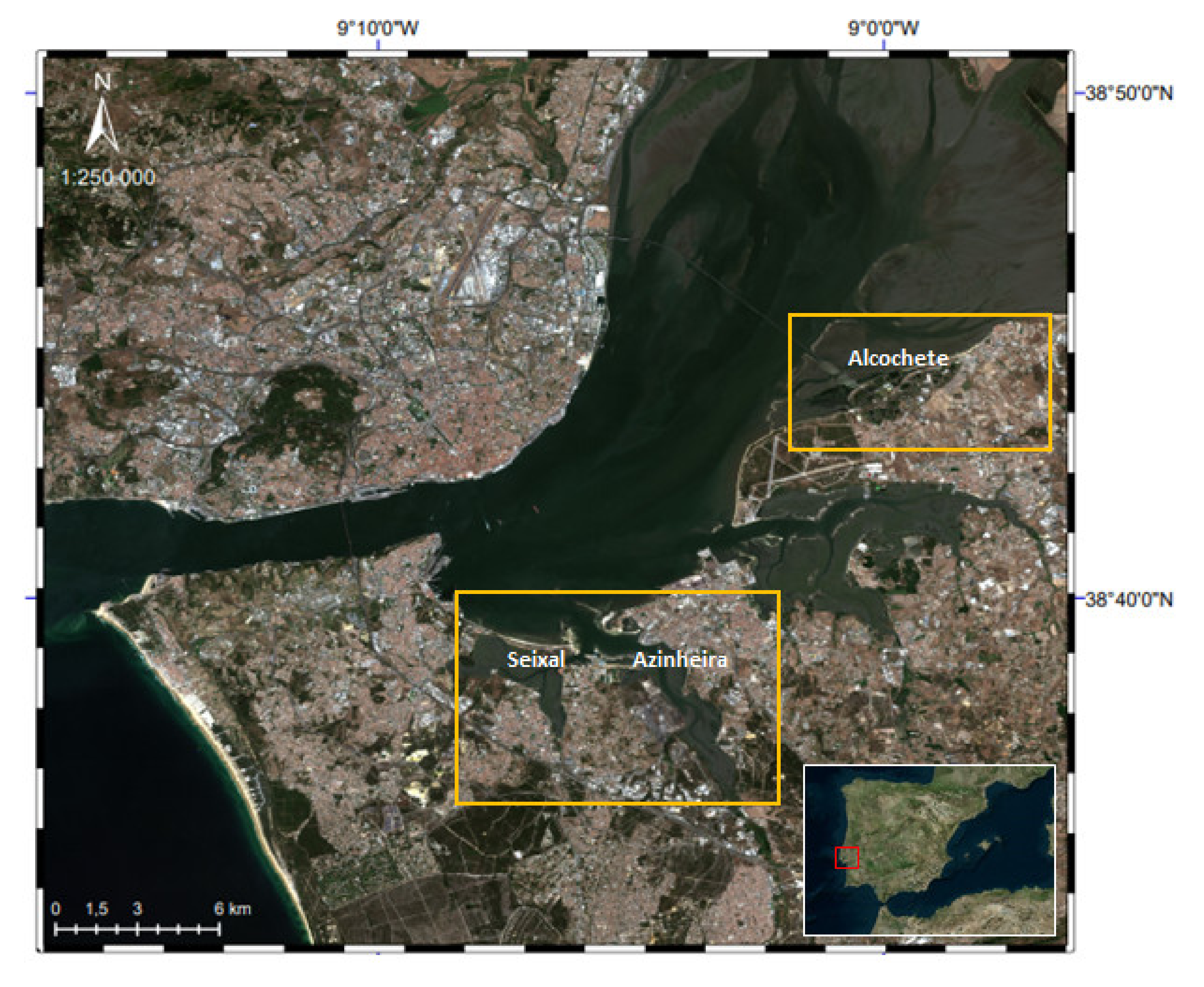
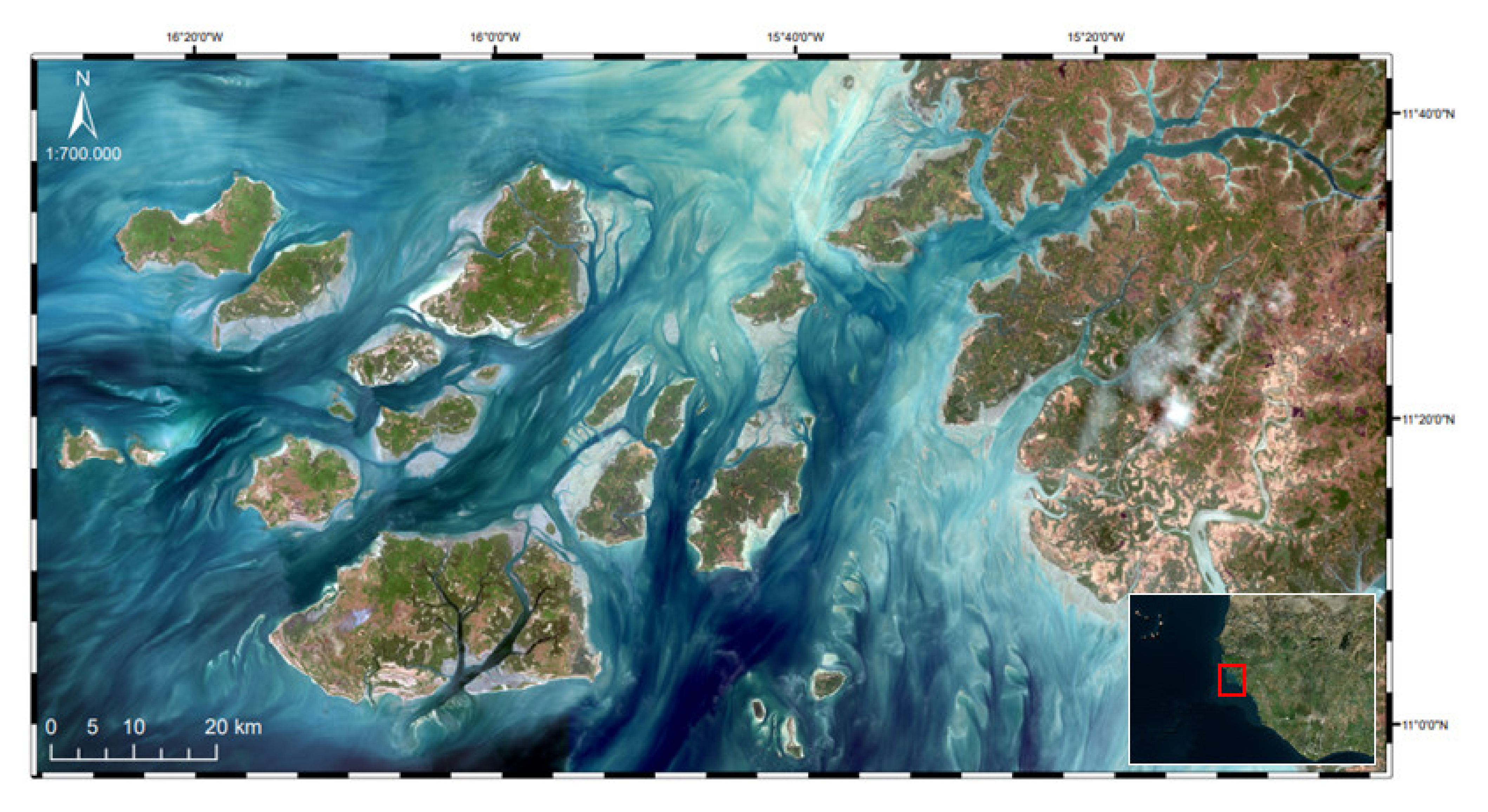
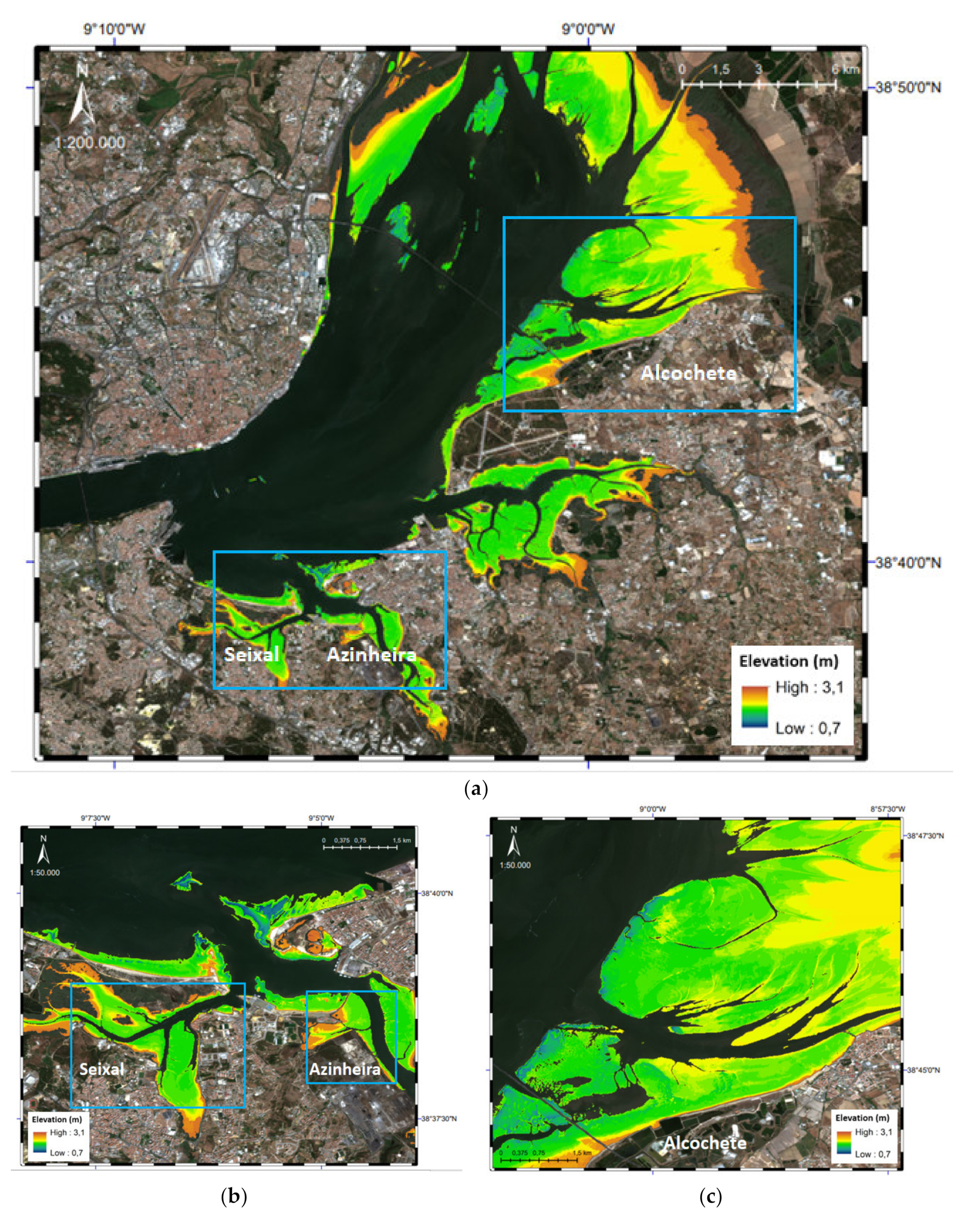
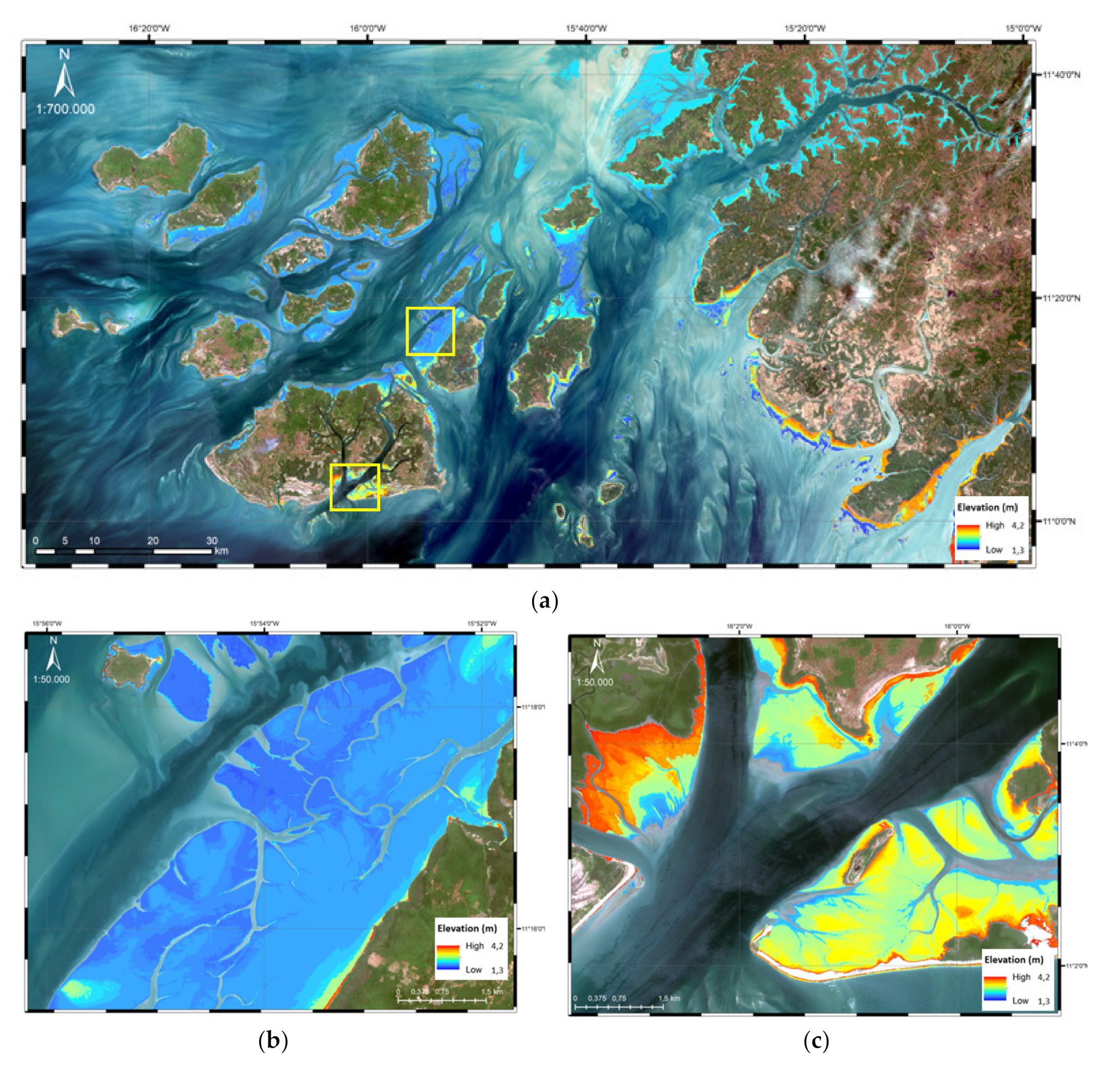
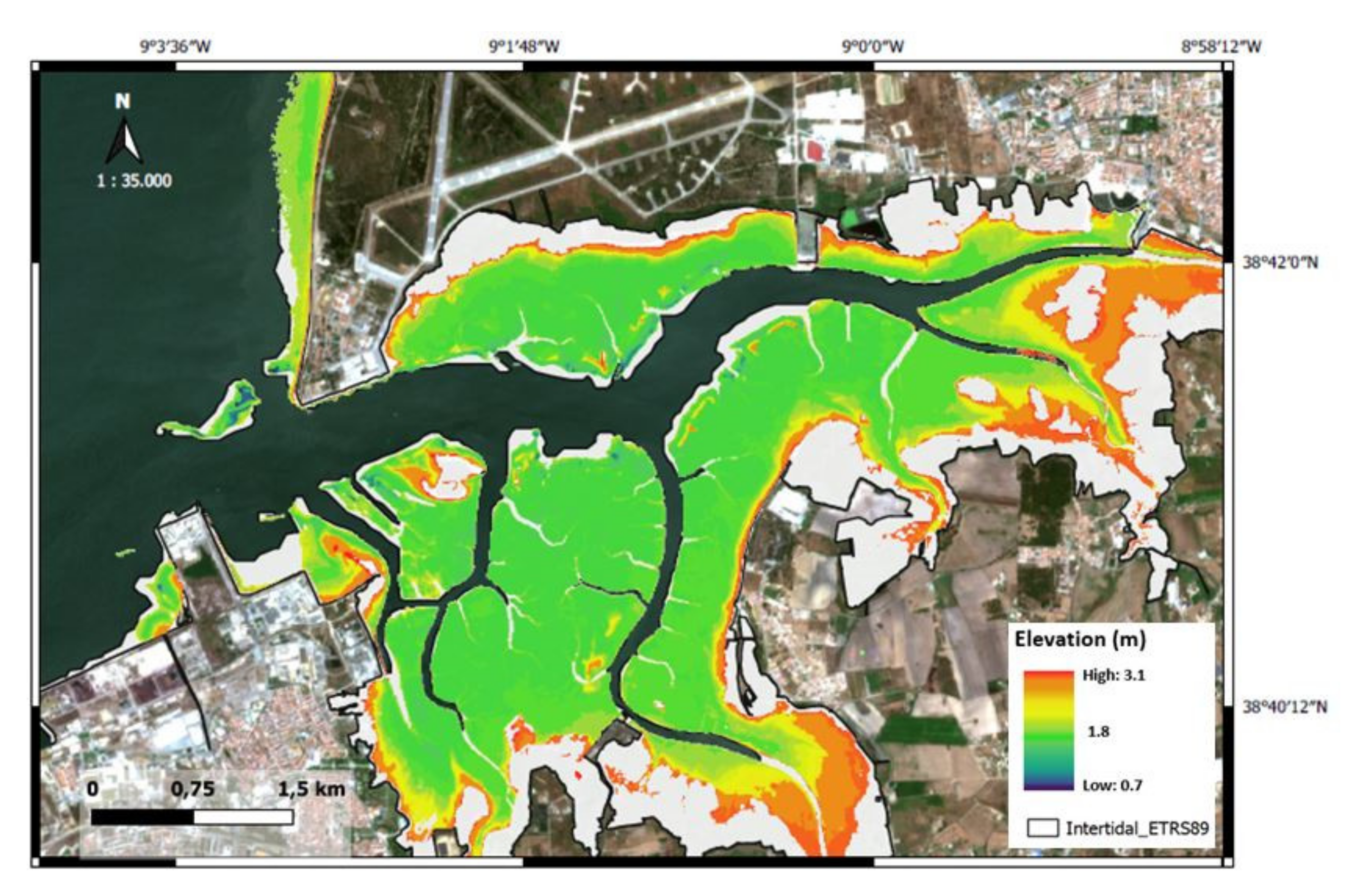
2.1. Study Areas

Two study areas with different optical water column characteristics and different geographic and morphological frameworks, were selected to test the bathymetry retrieval algorithm. The two study areas are: the Tagus river estuary, in Lisbon, Portugal, in West Europe, and the Bijagós archipelago, in Guinea-Bissau, in West Africa. The Tagus is the largest river of the Iberian Peninsula, ending in a large tidal estuary covering an area of 320 km2. The Tagus estuarine surface is characterized by extensive tidal flats, salt marsh vegetation and mudflats, where 40% of the estuarine area is intertidal [2,5,36] (Figure 1). The depths in the Tagus estuary vary between 2 m in the northern part that includes most mudflats, the middle part with average depths of 7 m, and 46 m in the downstream sections at the main navigation channel [5,36]. The Tagus estuary is mesotidal (tidal range between 2 and 4 m) with a maximum amplitude of 3.9 m and has a semidiurnal tide regime [32,36].
The Bijagós archipelago, located in the Tropical Atlantic Ocean, 12 miles west of Guinea-Bissau mainland, has 88 islands and islets and was classified in 1996 by the United Nations Educational, Scientific, and Cultural Organization (UNESCO) as a biosphere ecological reserve [37,38]. This archipelago, where the continental estuaries and coastal currents from Guinea and the Canaries meet, is characterized by extensive sandbanks, mangroves, intertidal areas, sandy beaches, and shallow water channels [4,37,38]. About 16% of the 10.000 km2 belonging to the Bijagós archipelago area is intertidal zone [38] (Figure 2). Bijagós has a semidiurnal tide regime and is also meso-tidal, with maximum amplitudes of 4.3 m [32,36].

2.2. Satellite Images
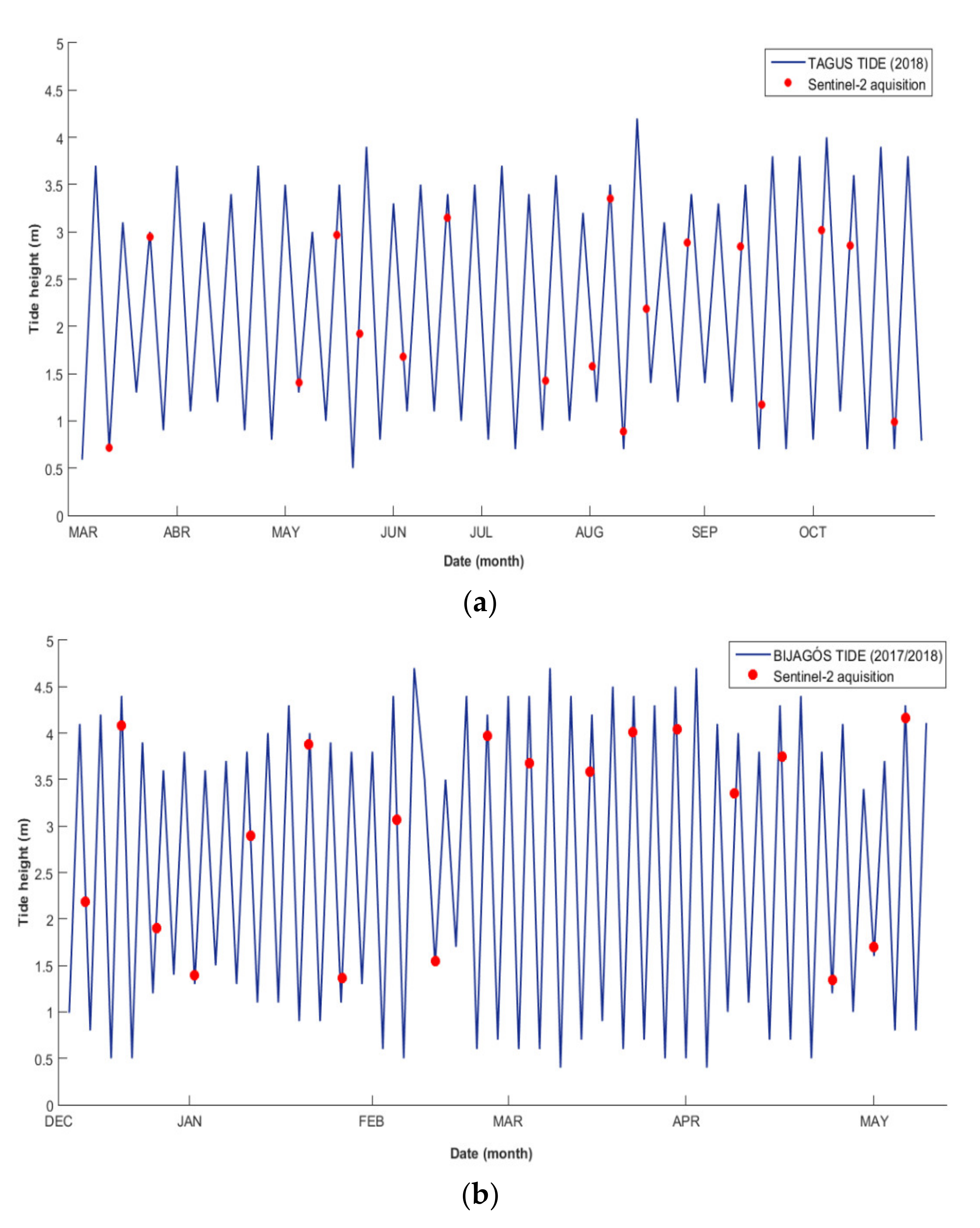
A set of 18 and 19 multispectral images from Sentinel-2 A&B (S2A and S2B), over the Tagus and Bijagós, respectively, were used in this work (Table 1). S2 A&B Level-1C (L1C) products were downloaded from the Sentinel’s Scientific Data Hub [39]. The images are georeferenced in WGS84/UTM 29N (Tagus) and 28N (Bijagós) time zones [40,41]. The images were acquired between March and October 2018 in the Tagus estuary (Table 1a) and between December 2017 and May 2018 in the Bijagós archipelago (Table 1b). Atmospheric correction is considered a critical step for the analyses of multispectral satellite images, especially for multitemporal images and to improve the accuracy of the bathymetric models produced [42,43,44,45]. S2 images were processed to Level-2A (L2A) with the ACOLITE free processor developed by the Royal Belgian Institute of Nature Sciences (RBINS) [46]. This atmospheric correction processor, which supports Landsat (5/7/8) and S2 (A/B) images, was designed specifically for aquatic applications, generating output products from several parameters derived from water reflectance [46,47,48,49,50]. The processed ACOLITE products used in this work correspond to the surface reflectance ( ρ s ) in all visible and Near InfraRed (NIR) bands, resampled to 10 m pixel size [46]. The Remote Sensing Reflectance (Rrs) algorithm available in this processor extensively used by the remote sensing community [43,46,49,51,52] is not suitable for intertidal areas once the land pixels are masked out by the algorithm. To decrease inter-pixel variability and some noise in the images, a spatial filter (median—3 × 3 filter) was applied on the different bands. Recent works with S2 images proved that spatial filtering can enhance bathymetric products [45,51,52]. Snap 6.0, Matlab R.2018a, ArcGIS 10.3.1, CARIS 4.4.3, and ACOLITE (version 20190326.0) were used for processing satellite data and image visualization.

2.3. Tide Data

The tide height for Bijagós was extracted from tidal model predictions of the Portuguese Hydrographic Institute (IH—Instituto Hidrográfico) [32]. For the Tagus estuary, the tide height was extracted from a tide gauge located in Lisbon harbor. The tide height tide at the acquisition time of the Sentinel-2 images is presented in Table 1.
Figure 3 shows the tide heights at Tagus estuary (a) and at Bijagós (b). The red dots are plotted according to S2 acquisition time, which in the image dataset corresponds to 11:21 UTC. It is observed that at the Bijagós, most of the images are acquired during high tide. This could be a limitation on the representation of the intertidal model since the acquired images do not cover accurately the intertidal area dynamics. However, this apparent limitation can be overcome by extending the period of the images acquisition, as in studies that have used 30 years of Landsat images [24].

2.4. In Situ Data for Validation

In July 2018, a hydrographic survey was conducted in the Tagus estuary at Azinheira area (Figure 4). A high-resolution bathymetric model at 1 m resolution was generated and was selected as reference data set for the Tagus area [53]. The range of depths within this data set is 3.10 m (only covers with high tide values) to −7.19 m maximum depth. Standard chart datum was used as reference as well. This data set was gridded at the S2 resolution (10 m) through the CARIS bathymetric processor.
For the Bijagós archipelago, the only official data available for bathymetric models validation are the information displayed in the nautical charts of Guinea-Bissau and Bijagós archipelago [54]. These official documents are the only available information that can be used as reference data, although the bathymetric information dates back to 1950/1960. According to the International Hydrographic Organization (IHO), 70% of the world coastal areas are not adequately surveyed or a re-survey is urgently required [55]. Guinea-Bissau and the Bijagós archipelago it is not an exception (Figure 5).

3. Methods

Estuarine regions are characterized by a low relief and reduced bottom slope, with several muddy small channels and generally with sparse vegetation [5,36] The areas exposed to the tidal regime, such as estuaries and beaches, are flooded once or twice a day at different water heights, according to the local tide cycle. The surface exposed to the tidal regime, the intertidal zone, has a variable spectral reflectance in one tidal cycle. The spectral reflectance differences are clearly seen with strong absorption of the infrared radiation in high tides and moderate reflection in low tide. The near infrared reflectance amplitude is a function of vegetation or algae density in the intertidal zone [33,43,51]. The proposed technique is based on the premise that the surface reflectivity variation in the NIR-band, over a time series of multispectral images, is related to the surface elevation and tide height. During one tide cycle, the lower intertidal zone (lower elevations) is covered by water for longer periods than the upper zone (higher elevations) which is more exposed to sunlight. Therefore, the lower intertidal zone would have a lower NIR reflectivity over a long period than the upper intertidal zone. Thus, it is reasonable to assume that at intertidal zones, NIR reflectivity is related to the surface elevation.
Regarding the bathymetry extraction, the time series of the multispectral images should be relatively short to prevent any changes in morphology. We assumed that soil roughness and local vegetation do not have significant changes during the time window of this study. The proposed method is divided in four steps: (1) Preprocessing; (2) Intertidal zone pixels selection; (3) Logistic regression; and (4) Derivation of the bathymetric model.

3.1. Preprocessing

The preprocessing phase aims to prepare all chosen or available images of the dataset. First of all, the atmospheric correction is made through the ACOLITE processor in order to convert the L1C top of atmosphere reflectance ( ρ T O A ) into bottom of atmosphere surface reflectance ( ρ s ) [46]. Then all images are reprojected into the UTM/WGS84 respective time zone. The image acquired at the lowest tide is selected as the reference image for the coregistration.

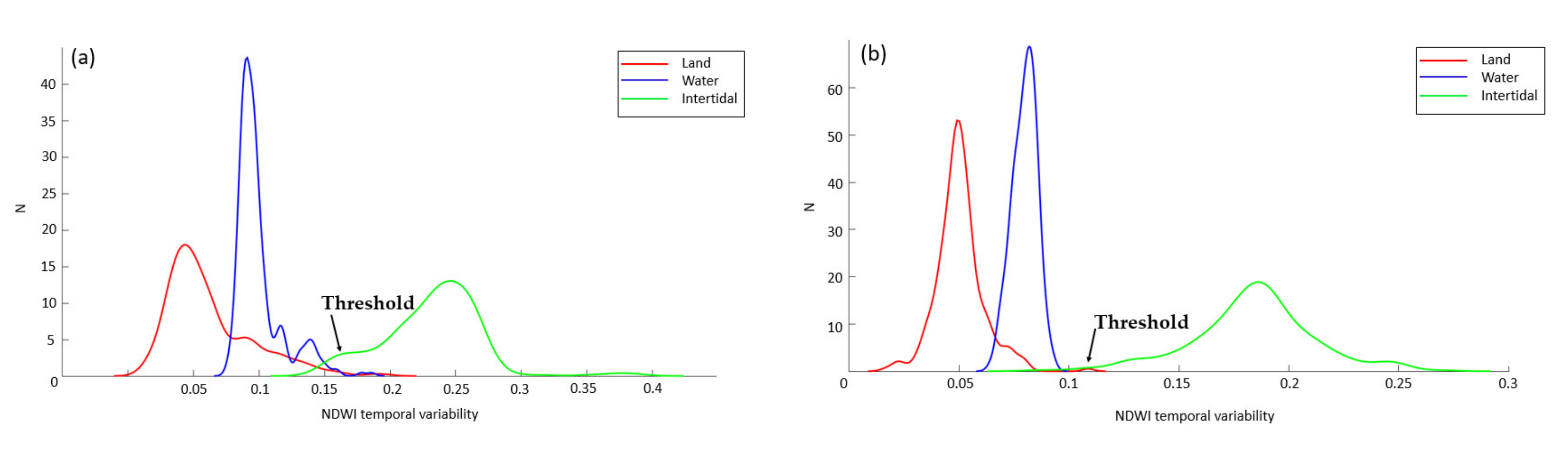
3.2. Intertidal Zone Pixels’ Selection

The first step of the algorithm consists of the identification of the intertidal zone on the multispectral image. For that, the Normalized Difference Water Index (NDWI) is used. The NDWI allows the discrimination of water pixels from land pixels, setting a locally adjusted threshold [56]. The NDWI is based on the normalized ratio between the green and the NIR bands (Equation (1)):
N D W I = G r e e n N I R G r e e n + N I R
The Temporal Variability (TV) analysis of the NDWI is used to discriminate different soil types and is given by:
σ x ,   y = 1 M i = 1 M N D W I i N D W I ¯ 2
where N D W I ¯ is the NDWI temporal mean of each pixel (x,y). As the intertidal zone is our area of interest, we used the TV parameter to discriminate 3 different classes of soil occupation—intertidal zone, land (beach berm/dry sand), and water. The intertidal class can be discriminated based on the high TV of the NDWI, as compared to the other two classes. The water class is characterized by a low TV and a high value for the NDWI, when compared with the intertidal zone. The beach berm (land) class has also a low TV, but it is expected that the value for NDWI, contrary to the water class, is smaller than the intertidal zone. The principal and distinguished characteristic of the intertidal zone is a higher TV value. The proposal is to use the TV as a threshold to identify the pixels belonging to the intertidal zone. If there is a slight overlap between classes, the threshold should be selected maximizing the number of intertidal pixels. The selected pixels in the intertidal zone or nearby are considered as candidate pixels for the next phase—the logistic regression analysis. If some overlap between the three classes exists, some water and land pixels will also be considered as candidates. The candidate pixels’ selection aims to reduce the number of pixels to be analyzed in the logistic regression. Therefore, it will always be preferable to have candidate pixels in excess, knowing that some of these pixels are going to be excluded in the logistic regression analysis.

3.3. Logistic Regression

The logistic regression is used to explain the relationship between the intertidal surface reflectance in the NIR spectral band and the tide height and to predict the elevation of the surface relative to the chart datum (hydrographic reference). We have noted that, when properly ordered by the tide height, the reflectance values at intertidal zones follows a sigmoid curve (Figure 6a). High reflectance is expected for low tides, and low reflectance is expected for high tides. We propose the following function to explain the relation between the height of a pixel and its reflectance:
ρ i x , y = k 1 + e a h i h t + L o w L i m i = 1 , , M
where for each pixel, (x,y) are the image coordinates, h t corresponds to the elevation of the pixel (x,y), h i is the tide height, and ρ i is the corresponding NIR reflectance. The logistic function is characterized by two parameters: a and k, where the steepness is correlated with the parameter a. The function will increase if a is positive and will decrease with tidal height ( h i ), when a is negative. The logistic function superior asymptote is correlated with the k value. The shape of the logistic function is tuned by these parameters, and they are estimated through adjustment with each pixel reflectance. The LowLim in Equation (3), related to the lower asymptote, could be a third parameter to characterize the logistic function. However, this parameter is not related with the shape of the sigmoid and will be neglected in the following analysis. In fact, the correlation between the tide height and the time variable reflectance is described only by the other two parameters. The sigmoid function is shown in Figure 6a for a range of steepness values. According to our experience, the steepness parameter a must be in the range −10 m−1 to −2 m−1.
The logistic analysis purpose is to achieve the parameters a and k and predict the surface elevation ( h t ). The a parameter can be defined through the tide regime and topography, reducing the number of parameters to be estimated. As the function is not linear, the terrain height h t   and the parameter k are obtained by searching in the bi-dimensional space of the minimum solution of the cost function:
E = i = 1 M h i h t + 1 a l n ρ i k ρ i 2
The number of images in the dataset (M), the different tide heights registered, and the tide amplitude are factors that contribute to the accuracy of the estimated pixel altitude. The logistic regression is applied to all candidate pixels, and as a result, the cost function and each pixel height are predicted. The two-dimensional problem can be converted to a one-dimensional problem, assuming that k is the maximum reflectance. Hence, the pixel’s height is predicted by searching in the one-dimensional space (local tide range) of the minimum solution of the cost function. The cost function for a range of steepness values is shown in Figure 6b. We observe that the steepness value is not relevant for the predicted height. In fact, the predicted height range is 2.51 to 2.60 m, changing the steepness value from −2 m−1 to −10 m−1, and the cost function minimum ranges from 0.012 to 0.04 (reflectance).
Regardless of the pixel classification (land, water, intertidal zone), the pixel height is estimated within the low and high tide of the area. Therefore, a false altitude value could be predicted for pixels not belonging to intertidal areas. These pixels are not likely to have a sigmoid shape behavior, and the logistic regression will return a large error. Instead of using a threshold based on the cost function error, we propose a geometric approach. A shape index of the logistic curve, the saturation index, was used to detect and select the pixels belonging to the intertidal class. This index allows for discrimination of the true S-shape logistic function from a flat function that does not reflect the correlation between reflectance and tide height, expected for intertidal zones. The saturation index is defined as:
s a t = ρ m a x ρ m i n ρ m a x + ρ m i n
where ρ m a x and ρ m i n are the values for the maximum and minimum asymptotes of the logistic curve, respectively. The saturation index can be used to remove the pixels with a low correlation between the reflectance and the tide height.

3.4. Derivation of the Bathymetric Model

The logistic regression output is a 3D point cloud with a set of georeferenced points (latitude, longitude, and elevation), in reference to the WGS84 geodetic system and, for elevation, in reference to the local tide system (chart datum) or mean sea level. For the Tagus estuary, the reference level (hydrographic reference) is 2.08 m below the mean sea level [32]. For the Bijagós archipelago, the hydrographic reference is 2.54 m below the mean sea level [32]. The 3D point cloud output is then interpolated using the inverse distance function, generating a regular grid of elevations of the intertidal surface. The quadrant search method with a 20 m radius (twice the cell resolution) was used to select the observations. A blank node criterion was applied when we have pixels with more than two quadrants without observations. The final spatial resolution of the Digital Elevation Model (DEM) is 10 m.
The accuracy of the logistic regression method was assessed using in situ data, hydrographic surveys [53], and chart depths [54]. The statistical data and error estimation are presented later in this paper.

3.5. Log-Transformed Ratio Bands Bathymetric Models

The derived intertidal elevation model according to the proposed methodology is also compared with other methodologies based on satellite multispectral images. There are many techniques, methods, or methodologies for bathymetry derivation from satellite images, such as the already mentioned empirical ratio log-transformed algorithm [30] and simple physically-based algorithm [29], as well as others specific for river bathymetry extraction, such as the Optimal Band Ratio Analysis (OBRA) [57] or the Multiple Optimal Depth Predictor Analysis (MODPA) [58]. One of the most widely used methods for satellite-based bathymetry derivation is the ratio transform model [30] [12,17,26,42,43,51,52,59]. This algorithm has good performances in shallow, turbid, and reef waters [23,24,42,51,59]. The model empirically derived the relationship between the changing ratio of two water-penetrating waveband pairs and the water depth, independently of the bottom albedo [18,30]. This band-ratio model was developed using the basic principle of the water body’s absorption level delivered by every band. The diversity level of the water body’s absorption theoretically will produce the ratio between bands. The empirical solution results from the natural logarithm ratio of two spectral bands reflectance, and the ratio produces a linear response with depth [30,42,52]. The model was designed to operate in clear waters, using a very small number of empirical coefficients and only needing a limited number of in situ measurements for calibration, which makes this methodology simpler to apply [18,42,43].
The model is given by the following expression (Equation (6)):
h x , y = m 1   l n   n   ρ s λ i l n n   ρ s λ j m 0
y = m 1 x m 0
where ρ s λ i is the surface reflectance of the blue band, ρ s λ j the surface reflectance of the red band, and m 1 and m 0 are the tunable constants to linearly transform the bands ratio to depths. The gain factor ( m 1 ) provides the relationship between the ratio and the in situ depth values (h), and the offset ( m 0 ) is the deviation from the zero depth (h = 0). These constants are estimated from the regression line between the logarithm ratio and the in situ measurements (Equation (7)). In Equation (6), h is the satellite derived depth (in meters) at x , y pixel position. n is a fixed constant applied to ensure positive logarithms under any condition. This constant will also assure that a residual non-linearity in the ratio is removed from depths that are retrievable from satellite and usually take values between 500 and 1500 [30]. We used n = 1000 in this study.

4. Results

4.1. Pre-Processing

The Sentinel-2 images were atmospherically corrected using the ACOLITE software and coregistered to a reference image. The reference image was the image with lowest tide. The reference image for the Tagus estuary was acquired on the 21 March 2018 and at Bijagós on the 25 April 2018. As the risk of image saturation by sun glint effects is too high on the intertidal zone, preliminary tests were made on the identification of the improvement using the sun glint correction [60]. We have verified that that sun glint correction did not improve the results, and in some cases, a degradation on the quality of the images was observed. Thus, no sun glint correction was applied to the Sentinel-2 images. The NDWI index was computed for all images. For each Sentinel-2 multiband image, a subset of two images was used in the algorithm: the NDWI and the NIR (band 8). The problem in using the NIR band is related with the presence of turbidity and seaweed or marine debris on the low intertidal area on the ebb tide. However, the NIR can be effective on the middle or upper intertidal area [35]. The Short Wave InfraRed (SWIR)band shows more problems than the NIR, and the most sensitive to the location of the waterline is the thermal IR [34]. Regarding the suspended organic matter or turbidity in shallow waters, red-edge bands are suitable for monitoring [25,43,51].

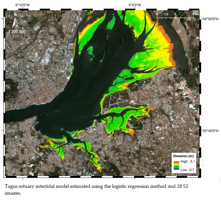
4.2. Intertidal Model Estimation

The temporal variability (TV) of the S2 images was computed using the standard deviation of the NDWI. The temporal variability of the NDWI in the northeast of the Tagus estuary and the Formosa, Maio, and Ponta islands at Bijagós, are presented in Figure 7.
As expected, the intertidal area and the agricultural fields display a high TV and hence higher intensity values. The dark pixels are characterized by low NDWI TV and are associated with water surfaces or land. The candidate pixels are pixels selected from the Standard Deviation (STD) TV map (Figure 7) according to the threshold values provided by the analysis of the TV histogram. The NDWI TV for the water, land, and intertidal pixels (3 classes) is presented in Figure 8. The intertidal class is discriminated based on the high NDWI TV, comparatively to the other two classes. The water class is characterized by a low TV and a high value for the NDWI, when compared with intertidal areas. Land class has also a low TV, but it is expected that the value for NDWI, contrary to the water class, will be smaller than the intertidal zone. The principal and distinguished characteristic of the intertidal zone is a higher TV value. The histogram shows well defined classes, and a good choice for intertidal zone threshold is 0.16 for Tagus estuary and 0.11 for Bijagós. The definition of the threshold for the candidate pixels selection should reduce the pixel omission error at the intertidal zone. The candidate pixels are further analyzed using the saturation index.
Several intertidal models were computed to assess the algorithm sensitivity to different TV thresholds and saturation index values. The possible combinations of four different threshold values for each test area (0.15, 0.16, 0.17, and 0.18 for Tagus estuary (Table 2a) and 0.10, 0.11, 0.12, and 0.13 for Bijagós (Table 2b)) and three saturation indexes (sat = 0.2, 0.3, and 0.4) were compared with the electronic navigational charts which represent the test areas. The models that fits better the bathymetry represented in these charts were chosen, with the respective constant values (threshold and saturation index—red circles in Table 2). After the intertidal DEM reconstructions tests, we recommended values between 0.2 and 0.4 for saturation index. A reduction of the pixels’ quantity used to generate the DEM has been observed when increasing the TV threshold. Nevertheless, the tests show that the selection of a small TV threshold is not relevant, since the final number of pixels used to generate the bathymetric model is more influenced by the saturation index value (Table 2).
The generated intertidal elevation models for the Tagus estuary and for the Bijagós are presented in Figure 9 and Figure 10, respectively. The maximum and minimum elevations are limited by the highest and the lowest tide recorded in the image data set. A constant tidal height for the entire covered area was assumed, to simplify the calculations. An accurate pixel-wise tide model can be derived and used in the logistic function to improve the estimated pixel height [18,23,24,33,61], but that is beyond the scope of this study. The highest/lowest tide values were, respectively, 4.08 m/1.34 m for the Bijagós and 3.35 m/0.72 m for the Tagus estuary. Satellite images were acquired at 11:21 UTC for both study areas, limiting the measurement of the lowest annual tide, with values that could reach 0.3 m or 0.4 m, for Tagus estuary and Bijagós, respectively [32]. This limitation is not specific to this particular method, since any methodology that uses multitemporal satellite images will be conditioned by the satellite’s passage time [18,19,25,31,33].
In the two test areas, the intertidal elevation model reflects the small-scale morphology of the intertidal zone. All the morphologically relevant elements, such as the channels, dikes, and swamp and muddy areas are represented in the intertidal DEM and in agreement with the local morphodynamics [2,5,36,37,38]. At the Tagus estuary, the greatest differences were observed along the navigation channel borders, close to the largest bathymetric slopes (Figure 11). Even in the northern area of the Tagus estuary, the generated intertidal elevation model closely follows the updated official cartography available. There are some small differences regarding small silting and displacement of small sandbanks, which are characteristic of this area and occur every year [2,5,36]. The differences previously identified can be attributed to geolocation errors of the image and to the temporal difference between the satellite images and the validation data, especially for the Bijagós area. The areas with the highest elevation gradients are the most sensitive to positioning errors. At Bijagós, even though the bathymetric information dates back to the 1960s [54], the intertidal model generated fits well. Small differences between the model and the chart related to sandbanks and coastline contours are likely to be morphological changes suffered at Bijagós in the last 60 years [38]. However, in the finer details, some discrepancies can be noted. A few small sandbanks have disappeared or have slightly moved, but not in a significant way. All the small rivers and water streams are well defined and in accordance with the existing cartography for the area [54].

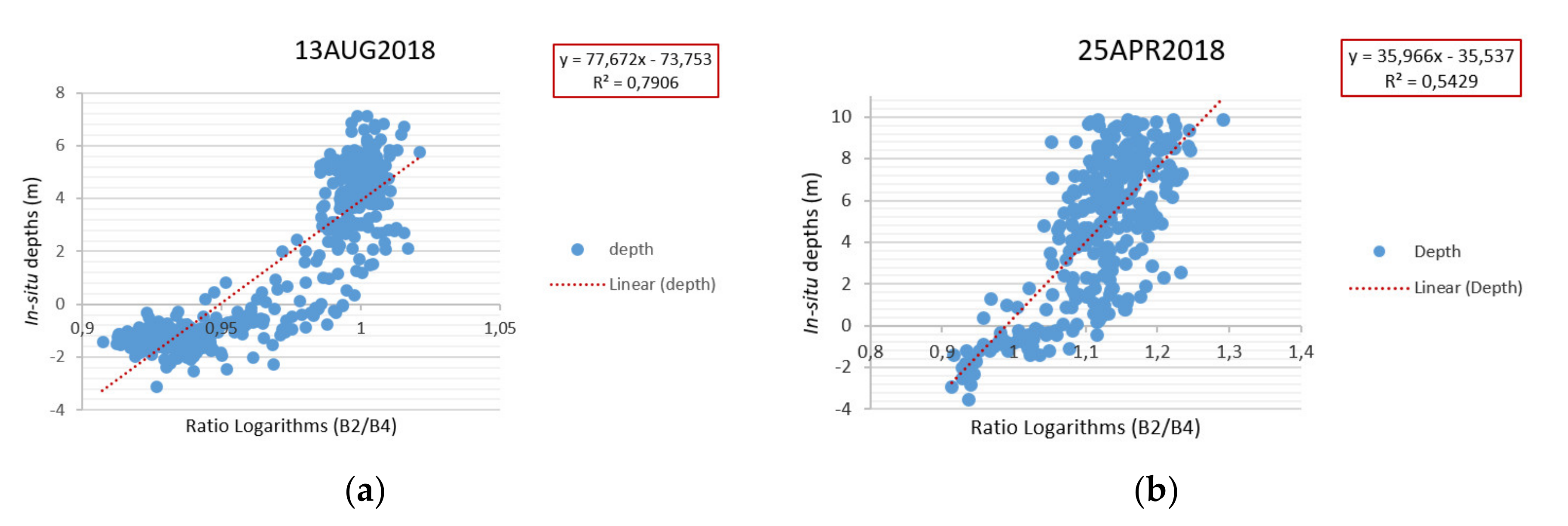
4.3. Logarithm Ratio Model Estimation

An additional intertidal elevation model was estimated for comparative purposes, using the logarithm ratio algorithm [30]. One S2 image was chosen for each site, and a sample of depth values were used to calibrate the model. The criteria for the selection of the images were the radiometric quality of the image and the tide height. Images acquired at high tide are preferred to estimate the intertidal zone. The images acquired on the 8th of August 2018 (3.55 m tide height) and on the 6th of December 2017 (4.08 m tide height) were used in the Tagus estuary and Bijagós, respectively. The model was calibrated with 507 and 78 depth values in both sites, selected from hydrographic survey in the Tagus estuary [53] and from a nautical chart in Bijagós [54]. Further details concerning the bathymetric model derivation with the ratio-transformed methodology [30,43,51] are presented in the Appendix A (Annex A). We confined the range of the calibration depths between 0 and 10 m (Figure A2) because the selected ratio bands presented best results in shallow waters [30,43,51,52].

4.4. Validation of the Models

The accuracy of the derived intertidal digital elevation models was assessed using a bathymetric survey in the Tagus estuary and depths extracted from a nautical chart in the Bijagós archipelago. Additionally, the derived intertidal elevation model was compared with the bathymetric model derived using the logarithm ratio method [30]. In the Tagus estuary, the hydrographic survey was performed by the IH in August 2018 (Azinheira) [53], and at the Bijagós, geolocated depths were selected from official nautical charts dating back to 1968, 1969, 1971, and 1982 [54].
The differences between the derived bathymetric model and the hydrographic surveys were computed, and the errors and accuracy assessments are shown in Table 3 and Table 4. The accuracy assessment of the logarithm ratio method-derived [30] elevation model is also presented. The achieved differences are limited to the tidal amplitude of the images time series, that is between 1.34 m and 4.08 m at the Bijagós, and 0.72 m and 3.35 m in the Tagus estuary (Figure 3). For this tidal range, the mean of the residues is −0.51 m and the standard deviation is 0.34 m for the Tagus estuary (Table 3). In the Bijagós the mean of the residues is −0.46 m and the standard deviation is 0.70 m (Table 4). As it was considered a constant tidal height for the entire covered area, these values could be reduced, taking into account that different geographic areas at the Tagus estuary have different tide height values for the same image acquisition time.
The logarithm ratio model [30] assessment was limited to the tidal amplitude used to validate the logistic regression model. The assessment gives high discrepancies between the predicted model and the ground truth, with an uncertainty of the order of 1.31 m and 1.26 m and a bias of 1.81 m and 4.8 m at the Tagus estuary and the Bijagós archipelago, respectively. The bias and the uncertainty are higher than the signal (the elevation), meaning that the algorithm is not appropriate for intertidal areas, although largely used for bathymetric prediction in areas with depths between 2 and 12 m [20].

5. Discussion

According to the results of our experiment, the two algorithms are complementary, with the logarithm ratio [30] performing better for depths higher than 2 m and the logistic regression performing better in the intertidal area, and can be properly merged to accurately model the near-shore bathymetry. At the Tagus estuary, the greatest differences were observed along the navigation channel borders, close to the largest bathymetric slopes. Even in the northern area of the Tagus estuary, the generated intertidal elevation model closely follows the updated official cartography available. There are some small differences regarding small silting and displacement of small sandbanks, which are characteristic of this area [2,5,36]. The differences previously identified can be attributed to geolocation errors of the image and to the temporal difference between the surveys and the satellite images. The areas with high elevation gradients are the most sensitive to positioning errors. At Bijagós, even though the bathymetric information dates back to the 1960s, the intertidal model generated fits well. Small differences between the model and the chart related to sandbanks and coastline contours are likely to be morphological changes suffered at Bijagós in the last 50 years. However, the estimated elevation can be improved assuming the spatial variability of the water level in the image. For this purpose, the local tide harmonic constants must be considered [32]. The tide height used in the work was assumed to have equal values across the entire study area, referred to the image acquisition time. The application of a modelled water level taking into account the tidal asymmetry over the Tagus estuarine area may improve the absolute accuracy of the model in future and provide a more realistic spatially varying water level distribution across the estuarine waters [18,31,33,36,61]. Likewise, it must be considered for each image acquisition time if the tide was progressing for a high or low tide situation and/or the presence of neap/spring tide, for a better accuracy of the DEM estimation. As there are no tide gauges at all desired locations, these factors will be considered for future works.
Regarding the fact that that about 70% of the world’s coastal areas are not adequately surveyed or a re-survey is urgently required, such as in Guinea-Bissau (Figure 5) [55], the methodology presented could fill the gap for intertidal areas, since the last surveys at Bijagós are from the 1960s. The application of our method to the Bijagós had presented a standard deviation of 70 cm at 10 m spatial resolution, but we believe that these values are related to the low accuracy of the reference elevation data, and the absolute accuracy of the model can be improved if this area were surveyed in future. The methodology described can also be useful for updating navigation charts, especially in intertidal or estuarine areas which have not been surveyed for many years, such the Bijagós archipelago.
This study has shown the potential of the logistic regression method for intertidal elevation extraction from S2 imagery. Atmospheric correction is crucial for a multitemporal study that uses multispectral images, reducing all the atmospheric effects that could influence the accuracy of the models [44,45,46,51,52,60]. Even so, the generated models can be affected by other sources of errors. According to [33,61], the vertical error of intertidal models is sensitive to the slope of the tidal flat. For the Tagus estuary area, the greatest differences of the model were observed close to the largest bathymetric slopes. The number of satellite images used also has an impact on the accuracy of the method [33]. The principle of waterline methods is to collect as many satellite images as possible because the tidal conditions are different in almost all of the images [18,31,33,34,61]. For this specific study, the number of images used can improve the accuracy of the DEM, especially if we used one image acquired at the lowest and at highest tide, normally during spring/neap tides, increasing the range of the bathymetric extracted values.
Regarding the novelty and the new findings of this method, the methodology is a pixel-by-pixel estimation for intertidal depths, presenting higher density of measurements than other waterline methods [31,33,61]. It can be applied to SAR (with adaptations to the backscattering) or multispectral images with low manual processing. The principal advantage of this method to be applied on multispectral images, rather than SAR images [19], is that the preprocessing phase of the method is more complex in order to coregister, calibrate, and despeckle SAR images. The logistic regression showed also another disadvantage when applied to SAR images. The DEMs generated have more pixel information gaps at intertidal areas than when applied to multispectral images [62].
Other authors, using different approaches, have reached similar intertidal elevation model accuracy. Regarding the shallow water areas, some retrieval bathymetry models with an accuracy of 0.89 m (0–12 m depth) [20]; 0.62 m with linear band model; and 0.81 m with log-transformed band ratio model, both at 2–6 m depth [42], near our results with the blue/red logarithm ratio model. At intertidal zones, other studies presented better results, such as those using the waterline method principles achieving models with accuracy of 10.9 cm root-mean-squared error, and as in our method, the key to obtaining accurate intertidal models is the number of images that can be used and the accuracy of the reference elevation data [35]. Additionally, other discussed methods had presented similar results. The temporal waterline radar method [31] that provides a map of the elevation of the waterline relative to the tidal reference, has an accuracy that varies from 12 cm to 50 cm, depending on the distance from the radar. The accuracy of the method presented by [23,24] are also similar to our results. They presented the first continental scale application that derives a relative elevation profile and topography of Australia’s vast exposed intertidal zone at 25 m spatial resolution through a combination of global tidal modelling with a 30-year time series archive of spatially and spectrally calibrated Landsat satellite data. The modelled elevations presented an accuracy of 41 cm for sandy beach, 39 cm for tidal flats environments, and least accurate values of 298 cm for rocky shores, reefs, and other complex coastal environments with extreme and variable tidal regimes.
The application of our method to the Bijagós presented a lower performance, but we believe that these values are related to the low accuracy of the chart datum and to the not recently updated hydrographic information of this area. The absolute accuracy of the model can be improved if this area were to be surveyed in future, like the IHO recommends [55]. The methodology described can also be useful for navigation charts updating, especially in intertidal or estuarine areas which have not been surveyed for many years, such the Bijagós archipelago.

6. Conclusions

In this study, an approach based on the logistic regression for deriving the intertidal bathymetry from multispectral images from Sentinel-2 A&B satellites was presented. The approach is based on the temporal variability of the near infrared spectral reflectance on the intertidal zone and the correlation with tide height. A logistic regression was used to model the temporal variability of the pixel’s reflectance and to minimize the cost function, and the pixel’s elevation was estimated. To remove the pixels that were wrongly classified as belonging to the intertidal class, a saturation index was suggested. This methodology can use multispectral images to extract an intertidal topo-bathymetric model automatically, not requiring the intervention of the operator. The atmospheric correction performed with the ACOLITE processor has retrieved surface reflectance values and improved the accuracy of the bathymetric models generated. It was observed that the number of satellite images used has an impact on the accuracy of the method and that the selection of the images must take into account the lowest and at highest tides, in order to increase the intertidal elevation range. The estimated intertidal morphology has a precision of 34 cm in the Tagus estuary and 70 cm in the Bijagós archipelago. The logistic regression method proved to reach better results for the intertidal areas when compared with the ratio transform algorithm, where the precision of the model was 1.32 m and 1.26 m for the Tagus estuary and the Bijagós intertidal zone, respectively. The proposed technique may contribute to generate digital elevation models of different intertidal and estuarine areas, mean sea level rise analysis, and flood hazard mitigation. Taking into account that there are coastal regions that have never been surveyed, or have not been surveyed for more than 50 years, such as the Bijagós archipelago, either due to financial reasons or because the areas are remote and inaccessible, this method can yearly update the intertidal bathymetric models with clear benefits to the nautical cartographic update.

Author Contributions

I.B. and J.C. conceived and designed the research. I.B collected and processed the remote sensing data, conducted the analysis and the validation and prepared the figures. J.C. reviewed and edited the writing and supervised the research. I.B. led the writing of the manuscript with contribution from J.C. and Á.S. All authors have read and agreed to the published version of the manuscript.

Funding

Isabel Bué’s PhD study is supported by the Portuguese Navy.

Acknowledgments

The authors would like to thank Instituto Hidrográfico for providing the cartographic, bathymetric, and tidal data. The Sentinel-2 images were obtained and downloaded from the Copernicus Open Access Hub.

Conflicts of Interest

The authors declare no conflict of interest.

Appendix A

ANNEX-A—Logarithm ratio model estimation
The best images in each test area were selected, under no cloud conditions, minimum sun glint, and closest to the lowest tide in the data set, to capture the extent of the intertidal area. All selected images were atmospherically corrected through ACOLITE processor and surface reflectance achieved (L2A images). We applied the equations of the ratio model (Equations (6) and (7)) to the values of the surface reflectance ( ρ s ) of the blue (B2 (490 nm)— λ i ) and red (B4 (664 nm)— λ j ) bands for each satellite image corrected for atmospheric effects. It is documented that using these specific ratio bands (blue/red) achieves optimal results in shallow waters (≤ 5 m) [43,51]. The authors also stated that for deeper shallow waters (10 m < depth < 18 m), the ratio blue/green performs better [30,43,51]. We tried both ratio bands, and we confirmed that the blue/red logarithm ratio performs better at intertidal areas (very shallow waters). We only present results from the bathymetric model generated through the blue/red ratio bands. We estimated bathymetry for several single images through the ratio band algorithm [30,43,51,52] in order to be compared with the intertidal models created from the logistic regression approach. The same authors stated that the ratio between blue/green bands presents worse results in shallow waters (≤ 3 m) [52] but optimal results for deeper areas (10 m–18 m). At a first stage, the blue/green ratio was used to create these bathymetric models, but as expected, they retrieved models with a very bad overall precision (STD = 2.15 m for Tagus estuary and STD = 4.27 m for Bijagós). After that, we created the logarithm ratio models through the blue/red ratio bands, and the results were improved [43,51,52]. Figure A1 shows the linear regression graphics that support Equations (6) and (7) of the model. The m 1 and m 0 are tuned by these linear regressions with the in situ depths. The correlation coefficient between the data sets is high for the Tagus estuary (R2 = 0.79). For the Bijagós archipelago, the correlation between the data sets was lower (R2 = 0.54), but the data used in this case for the calibration has not been updated since the 1960’s [54,55], and this could be a large source of error. Perhaps, the sample of depths used in this study for calibration (N = 500 for Tagus estuary and N = 307 for Bijagós) could be considered exaggerated. In fact, some authors defend that few calibration points were needed to calibrate the model, 5 to 10 [51] or 10 control points [43], because the model had only two parameters ( m 1 and m 0 ) that required tuning.
Figure A1. Linear regression graphics between in situ measurements (depths in meters) and the logarithm ratio. (a) Tagus estuary—13AUG18 S2A L2A image. (b) Bijagós archipelago—25APR18 S2B L2A image. (Red dashed line: linear regression best fit; red rectangle: correlation coefficient (R2) between data sets and Equation (7) solution).
Remotesensing 12 01311 g0a1
The logarithm ratio bands bathymetric models created are presented in Figure A2 and Figure A3. These models are not restricted to the tide height at image acquisition time because they are not a derivation of any waterline method. The only limiting conditions are dependence on the surface reflectance values retrieved after atmospheric correction and the tide height of the original image. Figure A2 shows the Tagus estuary bathymetric model (reference image—L2A S2A 08AUG2018), and more or less all the morphodynamics characteristics are represented. Figure A3 shows the bathymetric model for the Bijagós archipelago (reference image—L2A S2B 06DEC2017) and also fits well.
Figure A2. Bathymetric model for the Tagus estuary achieved through the logarithm ratio band algorithm. S2A L2A 08AUG2018 image.
Remotesensing 12 01311 g0a2
Figure A3. Bathymetric model for the Bijagós archipelago achieved through the logarithm ratio band algorithm. S2A L2A 06DEC2017 image.
Remotesensing 12 01311 g0a3
The range of the validation data sets covers all the negative soundings for the intertidal area that were not used for calibration proposes. The guarantee of the calibration and validation sample independence is very important in order to maintain the integrity of the model estimation [43,51]. The dimension of the validation data set in N = 507 for Tagus estuary and N = 78 for Bijagós. The logarithm ratio algorithm retrieved bathymetric models with an acceptable overall precision for the Tagus estuary. The model presented STD = 1.31 m, RMSE = 2.23 m, and bias = 1.81 m. For Bijagós, the model presented lower performance, with STD = 1.26m, RMSE = 5.00 m, and bias = 4.84 m. These values are inflated by the time difference between the satellite images and the chart depth information. This algorithm, with other applied corrections for turbid and coral reef waters, proved its value in retrieving bathymetric models from shallow waters (≤18 m) with typical errors ≤0.4 m [43], decreasing to 0.22m at depths ranging between 0–5 m [43,51,52]. The ratio band model, with further adaptations, could be appropriate for intertidal bathymetry derivation.

References

  1. Brito, A.C.; Moita, T.; Gameiro, C.; Silva, T.; Anselmo, T.; Brotas, V. Changes in the Phytoplankton Composition in a Temperate Estuarine System (1960 to 2010). Estuar. Coasts 2015, 38, 1678–1691. [Google Scholar] [CrossRef]
  2. Taborda, R.; Freire, P.; Silva, A.; Andrade, C.; Freitas, M.C. Origin and evolution of Tagus estuarine beaches. J. Coast. Res. 2009, 56, 213–217. [Google Scholar]
  3. Gameiro, C.; Cartaxana, P.; Brotas, V. Environmental drivers of phytoplankton distribution and composition in Tagus Estuary, Portugal. Estuar. Coast. Shelf Sci. 2007, 75, 21–34. [Google Scholar] [CrossRef]
  4. Wright, L.D.; Syvitski, J.P.; Nichols, C.R. Chapter 5: Coastal Morphodynamics and Ecosystem Dynamics. In Tomorrow’s Coasts: Complex and Impermanent; Wright, L.D., Nichols, C.R., Eds.; Springer: New York, NY, USA, 2019; pp. 69–84. [Google Scholar] [CrossRef]
  5. Guerreiro, M.; Fortunato, A.B.; Freira, P.; Rilo, A.; Taborda, R.; Freitas, A.C.; Andrade, C.; Silva, T.A.; Rodrigues, M.; Bertin, X.A.; et al. Evolution of the hydrodynamics of the Tagus estuary (Portugal) in the 21st century. J. Integr. Coast. Zone Manag. 2015, 15, 65–80. [Google Scholar] [CrossRef]
  6. Silva, A.N.; Taborda, R.; Antunes, C.; Catalão, J. Understanding the coastal variability at Norte beach, Portugal. J. Coast. Res. 2013, 65, 2173–2178. [Google Scholar] [CrossRef]
  7. Nerem, R.S.; Beckley, B.D.; Fasulto, J.T.; Hamlington, B.D.; Masters, D.; Mitchum, G.T. Climate-change–driven accelerated sea-level rise detected in the altimeter era. In Proceedings of the National Academy of Sciences, Toulouse, France, 25 February 2018; pp. 2022–2025. [Google Scholar] [CrossRef] [Green Version]
  8. Schuerch, M.; Spencer, T.; Temmerman, S.; Kirwan, M.L.; Wolff, C.; Lincke, D.; McOwen, C.J.; Pickering, M.D.; Reef, R.; Vafeidis, A.T.; et al. Future response of global coastal wetlands to sea-level rise. Nature 2018, 561, 231–234. [Google Scholar] [CrossRef]
  9. Bastos, A.P.; Ponte Lira, C.; Calvão, J.; Catalão, J.; Andrade, C.; Pereira, A.J.; Taborda, R.; Rato, D.; Pinho, P.; Correia, O. UAV Derived Information Applied to the Morphological Study of Slow changing Dune Systems. J. Coast. Res. 2018, 85, 226–230. [Google Scholar] [CrossRef]
  10. Silva, A.; Taborda, R.; Catalão, J.; Freire, P. DTM extraction using video monitoring techniques: Application to a fetch limited beach. J. Coast. Res. 2009, 56, 203–207. [Google Scholar]
  11. Bird, C.O.; Bell, P.S.; Plater, A.J. Application of marine radar to monitoring seasonal and event-based changes in intertidal morphology. Geomorphology 2017, 285, 1–15. [Google Scholar] [CrossRef] [Green Version]
  12. Chénier, R.; Faucher, M.; Ahola, R. Satellite-Derived Bathymetry for Improving Canadian Hydrographic Service Charts. ISPRS Int. J. Geo. Inf. 2018, 7, 306. [Google Scholar] [CrossRef] [Green Version]
  13. Dierssen, H.M.; Theberge, J.A.E. Bathymetry: Assessing Methods. Volume II Water and Air. Encyc. Nat. Res. 2014. [Google Scholar] [CrossRef]
  14. Quadros, N.D.; Collier, P.A. A New Approach to Delineating the Littoral Zone for an Australian Marine Cadastre. J. Coast. Res. 2008, 24, 780–789. [Google Scholar] [CrossRef]
  15. Wozencraft, J.; Millar, D. Airborne Lidar and integrated technologies for coastal mapping and nautical charting. Mar. Techno. Soc. J. 2005, 39, 27–35. [Google Scholar] [CrossRef]
  16. Jawak, S.D.; Vadlamani, S.S.; Luis, A.J. A Synoptic review on deriving bathymetry information using Remote Sensing Technologies: Models and Comparisons. Adv. Remote Sens. 2015, 4, 147–162. [Google Scholar] [CrossRef] [Green Version]
  17. Chénier, R.; Ahola, R.; Sagram, M.; Faucher, M.; Shelat, Y. Consideration of Level of Confidence within Multi-Approach Satellite-Derived Bathymetry. ISPRS Int. J. Geo-Inf. 2019, 8, 48. [Google Scholar] [CrossRef]
  18. Mason, D.C.; Davenport, I. Accurate and Efficient Determination of the Shoreline in ERS-1 SAR images. IEEE Trans. Geosci. Remote Sens. 1996, 34, 1243–1253. [Google Scholar] [CrossRef]
  19. Catalão, J.; Nico, G. Multitemporal backscattering logistic analysis for intertidal bathymetry. IEEE Trans. Geosci. Remote Sens. 2016, 55, 1066–1073. [Google Scholar] [CrossRef]
  20. Pacheco, A.; Horta, J.; Loureiro, C.; Ferreira, Ó. Retrieval of nearshore bathymetry from Landsat 8 images: A tool for coastal monitoring in shallow waters. Remote Sens. Environ. 2015, 159, 102–116. [Google Scholar] [CrossRef] [Green Version]
  21. Niedermeier, A.; Hoja, D.; Lehner, S. Topography and morphodynamics in the German Bight using SAR and optical remote sensing data. Ocean Dyn. 2005, 55, 100–109. [Google Scholar] [CrossRef]
  22. Schwäbisch, M.; Lehner, S.; Norbert, W. Coastline extraction using ERS SAR interferometry. In Proceedings of the 3rd ERS Symposium, Florence, Italy, 14–21 March 1997; pp. 1049–1053, Space Service Environment, ESA SP-414. [Google Scholar]
  23. Sagar, S.; Roberts, D.; Bala, B.; Lymburner, L. Extracting the intertidal extent and topography of the Australian coastline from a 28-year time series of Landsat observations. Remote Sens. Environ. 2017, 195, 153–169. [Google Scholar] [CrossRef]
  24. Bishop, -T.R.; Sagar, S.; Lymburner, L.; Beaman, R. Between the tides: Modelling the elevation of Australia’s exposed intertidal zone at continental scale. Estuar. Coast. Shelf Sci. 2019, 223, 115–128. [Google Scholar] [CrossRef]
  25. Pahlevan, N.; Sarkar, S.; Franz, B.A.; Balasubramanian, S.V.; He, J. Sentinel-2 MultiSpectral Instrument (MSI) data processing for aquatic science applications: Demonstrations and validations. Remote Sens. Environ. 2017, 201, 47–56. [Google Scholar] [CrossRef]
  26. Said, R.; Mahmud, M.R.; Hasan, R.C. Evaluating satellite-derived bathymetry accuracy from Sentinel-2A high-resolution multispectral imageries for shallow water hydrographic mapping. Available online: https://iopscience.iop.org/article/10.1088/1755-1315/169/1/012069/pdf (accessed on 24 April 2019).
  27. Lyzenga, D. Passive Remote-Sensing techniques for mapping water depth and bottom features. App. Opt. 1978, 17, 379–383. [Google Scholar] [CrossRef]
  28. Lyzenga, D.R. Shallow-water bathymetry using combined lidar and passive multispectral scanner data. Int. J. Remote Sens. 1985, 6, 115–125. [Google Scholar] [CrossRef]
  29. Lyzenga, D.R.; Malinas, N.P.; Tanis, F.J. Multispectral Bathymetry using a Simple Physically Based Algorithm. IEEE Trans. Geosci. Remote Sens. 2006, 44, 2251–2259. [Google Scholar] [CrossRef]
  30. Stumpf, R.P.; Holderied, K.; Sinclair, M. Determination of water depth with high-resolution satellite imagery over variable bottom types. Limnol. Oceanogr. 2003, 48, 547–556. [Google Scholar] [CrossRef]
  31. Bell, P.S.; Bird, C.O.; Plater, A.J. A temporal waterline approach to mapping intertidal areas using X-band marine radar. Coast. Engin. 2016, 107, 84–101. [Google Scholar] [CrossRef] [Green Version]
  32. Instituto Hidrográfico. Tabelas de Marés; Vol II Países Africanos de Língua Oficial Portuguesa e Macau; Instituto Hidrográfico: Lisbon, Portugal, 2018. [Google Scholar]
  33. Liu, Y.; Li, M.; Zhou, M.; Yang, K.; Mao, L. Quantitative Analysis of the Waterline method for Topographical Mapping of Tidal Flats: A case study in the Dongsha Sandbank, China. Remote Sens. 2013, 5, 6138–6158. [Google Scholar] [CrossRef] [Green Version]
  34. Ryu, J.-H.; Won, J.S.; Min, K.D. Waterline extraction from Landsat TM data in a tidal flat. A case study in Gomso Bay, Korea. Remote Sens. Environ. 2002, 83, 442–456. [Google Scholar] [CrossRef]
  35. Ryu, J.-H.; Kim, C.-H.; Lee, Y.-K.; Won, J.-S.; Chun, S.-S.; Lee, S. Detecting the intertidal morphologic change using satellite data. Estuar. Coast. Shelf Sci. 2008, 78, 623–632. [Google Scholar] [CrossRef]
  36. Neves, F. Dynamics and Hydrology of the TAGUS Estuary: Results from in Situ Observations. Ph.D. Thesis, Faculdade de Ciências da Universidade de Lisboa, Lisbon, Portugal, 2010. [Google Scholar]
  37. GUINÉ-BISSAU. A Reserva de Biosfera do Arquipélago dos Bijagós: Um Património a Preserver; Ministerio de Agricultura, Alimentación y Medio Ambiente de España, Administração da Guiné-Bissau: Bissau, Guiné-Bissau, 2012; p. 211. [Google Scholar]
  38. Carvalho, L.; Figueira, P.; Monteiro, R.; Reis, A.; Almeida, J.; Catry, T.; Lourenço, P.; Catry, P.; Barbosa, C.; Catry, I.; et al. Major, minor, trace and rare earth elements in sediments of the Bijagós archipelago, Guinea-Bissau. Mar. Pollut. Bull. 2018, 829–834. [Google Scholar] [CrossRef]
  39. Sentinel’s Scientific Data Hub. Available online: https://scihub.copernicus.eu/ (accessed on 8 March 2019).
  40. European Space Agency. Sentinel-2 User Handbook; ESA Standard Document; ESA: Paris, France, 2015; Available online: https://sentinel.esa.int/documents/247904/685211/Sentinel-2_User_Handbook (accessed on 12 June 2019).
  41. European Space Agency. Sentinel-2 MSI Technical Guide. 2017. Available online: https://earth.esa.int/web/sentinel/technical-guides/sentinel-2-msi (accessed on 18 June 2019).
  42. Casal, G.; Monteys, X.; Hedley, J.; Harris, P.; Cahalane, C.; McCarthy, T. Assessment of empirical algorithms for bathymetry extraction using Sentinel-2 data. Int. J. Remote Sens. 2019, 40, 2855–2879. [Google Scholar] [CrossRef]
  43. Caballero, I.; Stumpf, R.P. Towards routine mapping shallow bathymetry in environments with variable turbidity: Contribution of Sentinel-2A/B satellites mission. Remote Sens. 2020, 12, 451. [Google Scholar] [CrossRef] [Green Version]
  44. Vanhellemont, Q.; Ruddick, K. Atmospheric correction of metre-scale optical satellite data for inland and coastal water applications. Remote Sens. Environ. 2018, 216, 586–597. [Google Scholar] [CrossRef]
  45. Hedley, J.D.; Roelfsema, C.; Brando, V.; Giardino, C.; Kutser, T.; Phinn, S.; Mumby, P.; Barrilero, O.; Laporte, J.; Koetzh, B. Coral reef applications of Sentinel-2: Coverage, characteristics, bathymetry and benthic mapping with comparison to Landsat 8. Remote Sens. Environ. 2018, 216, 598–614. [Google Scholar] [CrossRef]
  46. Royal Belgium Institute of Natural Sciences. ACOLITE Python User Manual. 2019. Available online: https://odnature.naturalsciences.be/remsem/software-and-data/acolite (accessed on 27 January 2020).
  47. Vanhellemont, Q.; Ruddick, K. Turbid wakes associated with offshore wind turbines observed with Landsat 8. Remote Sens. Environ. 2014, 145, 105–115. [Google Scholar] [CrossRef] [Green Version]
  48. Vanhellemont, Q.; Ruddick, K. Advantages of high quality SWIR bands for ocean colour processing: Examples from Landsat-8. Remote Sens. Environ. 2015, 161, 89–106. [Google Scholar] [CrossRef] [Green Version]
  49. Vanhellemont, Q.; Ruddick, K. Acolite for Sentinel-2: Aquatic Applications of MSI Imagery. In Proceedings of the ESA Living Planet Symposium, Prague, Chez Republic, 9–13 May 2016. [Google Scholar]
  50. Ruddick, K.; Vanhellemont, Q.; Dogliotti, A.; Nechad, B.; Pringle, N.; Van der Zande, D. New Opportunities and Challenges for High Resolution Remote Sensing of Water Colour. In Proceedings of the Ocean Optics XXIII, Victoria, BC, Canada, 7 October 2016. [Google Scholar]
  51. Caballero, I.; Stump, P.R.; Meredith, A. Preliminary assessment of turbidity and chlorophyll impact on bathymetry derived from Sentinel-2A and Sentinel-3A satellites in South Florida. Remote Sens. 2019, 11, 645. [Google Scholar] [CrossRef] [Green Version]
  52. Caballero, I.; Stumpf, R.P. Retrieval of nearshore bathymetry from Sentinel-2A and 2B satellites in South Florida coastal waters. Estuar. Coast. Shelf Sci. 2019, 226, 106277. [Google Scholar] [CrossRef]
  53. Instituto Hidrográfico. Levantamento Hidrográfico Instalações Navais da Azinheira (Estuário do Tejo); Instituto Hidrográfico: Lisbon, Portugal, 2018. [Google Scholar]
  54. Instituto Hidrográfico. Cartas Náuticas do Arquipélago dos Bijagós Guiné-Bissau (223); Instituto Hidrográfico: Lisbon, Portugal, 1969. [Google Scholar]
  55. International Hydrographic Organization. IHO C-55 Publication Status of Hydrographic Surveying and Charting Worldwide, 2020, Monaco. Available online: https://iho.int/uploads/user/pubs/cb/c-55/c55.pdf (accessed on 17 February 2020).
  56. McFeeters, S.K. The use of the Normalized Difference Water Index (NDWI) in the delineation of open water features. Int. J. Remote Sens. 1996, 17, 1425–1432. [Google Scholar] [CrossRef]
  57. Legleiter, C.J.; Roberts, A.A.; Lawrence, R.L. Spectrally based remote sensing of river bathymetry. Earth Surf. Proc. Landf. 2009, 1787. [Google Scholar] [CrossRef]
  58. Niroumand-Jadidi, M.; Vitti, A.; Lyzenga, D. Multiple Optimal Depth Predictors Analysis (MODPA) for river bathymetry: Findings from spectro radiometry, simulations, and satellite imagery. Remote Sens. Environ. 2018, 218, 132–147. [Google Scholar] [CrossRef]
  59. Hamylton, S.M.; Hedley, J.D.; Beaman, R.J. Derivation of high-resolution bathymetry from multispectral satellite imagery: A comparison of empirical and optimization methods through geographical error analysis. Remote Sens. 2015, 7, 16257–16273. [Google Scholar] [CrossRef] [Green Version]
  60. Hedley, J.D.; Harborne, A.R.; Mumby, P.J. Simple and robust removal of sun glint for mapping shallow-water benthos. Int. J. Environ. 2005, 113, 2107–2112. [Google Scholar] [CrossRef]
  61. Mason, D.C.; Davenport, I.J.; Flather, R.A.; Gurney, C.; Robinson, G.J.; Smith, J.A. A sensitivity analysis of the waterline method of constructing a digital elevation model for intertidal areas in ERS SAR scene of eastern England. Estuar. Coast. Shelf Sci. 2001, 53, 759–778. [Google Scholar] [CrossRef]
  62. Bué, I.; Catalão, J.; Semedo, A. Intertidal Topo-bathymetry extraction from SAR and Multispectral images. In Proceedings of the Living Planet Symposium, Milan, Italy, 13–17 May 2019. [Google Scholar]
Figure 1. Tagus estuary in Lisbon. Red-green-blue (RGB) composite after atmospheric correction of Sentinel-2B imagery on 13 August 2018. The two orange rectangles identify specific intertidal areas at the Tagus estuary (top right—Alcochete and lower left—Seixal and Azinheira).
Remotesensing 12 01311 g001
Figure 2. The Bijagós archipelago in Guinea-Bissau. RGB composite after atmospheric correction of Sentinel-2B imagery on 25 April 2018.
Remotesensing 12 01311 g002
Figure 3. Tidal height variation: (a) Tide height at Tagus estuary from March to October 2018 and (b) Tide height at Bijagós archipelago from December 2017 to May 2018. The red dots represent the Sentinel-2 images dataset (time—11:21 UTC).
Remotesensing 12 01311 g003
Figure 4. Bathymetric model acquired by hydrographic survey in Tagus estuary—Azinheira area (red: 3.1 m above chart datum and green: 7.2 m below chart datum).
Remotesensing 12 01311 g004
Figure 5. Guinea-Bissau status of hydrographic surveying in accordance with International Hydrographic Organization (IHO) information (adapted from IHO [55] (p 215)).
Remotesensing 12 01311 g005
Figure 6. (a) NIR reflectance time series as a function of the tide height (red circles) and adjusted sigmoid function for a range of steepness parameters (from −2 to −10) and (b) cost function for a range of steepness values.
Remotesensing 12 01311 g006
Figure 7. Normalized Difference Water Index (NDWI) temporal variability: (a) Alcochete area in Tagus estuary and (b) Formosa, Maio, and Ponta islands at Bijagós archipelagos.
Remotesensing 12 01311 g007
Figure 8. NDWI temporal variability of the three classes: water (blue), intertidal (green), and land (red); (a) Tagus estuary and (b) Bijagós archipelago.
Remotesensing 12 01311 g008
Figure 9. (a) Tagus estuary intertidal model estimated using the logistic regression method and 18 S2 images (red: 3.1 m and dark blue: 0.7 m). The two blue rectangles highlight specific intertidal areas at the Tagus estuary (bottom left—Seixal and Azinheira; top right—Alcochete), (b) zoom on the intertidal model estimated for the Tagus estuary—Seixal and Azinheira areas, and (c) zoom on the intertidal model estimated for the Tagus estuary—Alcochete area.
Remotesensing 12 01311 g009
Figure 10. (a) Bijagós intertidal model estimated from 19 S2 images (red: 4.2 m and dark blue: 1.3 m). The two yellow rectangles highlight different intertidal areas; (b) zoom on the intertidal model estimated for the Bijagós (top right rectangle in (a)—sandy beaches); and (c) zoom on the intertidal model (bottom left rectangle in (a)—mostly mangroves and mudflats [37,38]).
Remotesensing 12 01311 g010
Figure 11. Comparison between derived intertidal model in Tagus estuary and cartographic intertidal area shown in white. Greatest differences are observed along the navigation channel due to intense maritime traffic in the area.
Remotesensing 12 01311 g011
Table 1. List of Sentinel-2 A&B images used in this study for intertidal bathymetry extraction. Tide height (m) corresponding to image acquisition time (11:21 UTC). (a) Tagus estuary and (b) Bijagós archipelago.
NumberDateSensorTide Height (m)
(a)
121 March 2018S2A0.72
226 March 2018S2B2.95
305 May 2018S2B1.40
410 May 2018S2A2.97
515 May 2018S2B1.92
619 June 2018S2A1.68
724 June 2018S2B3.15
829 July 2018S2A1.43
903 August 2018S2B1.58
1008 August 2018S2A3.35
1113 August 2018S2B0.89
1218 August 2018S2A2.19
1323 August 2018S2B2.89
1422 September 2018S2B2.84
1527 September 2018S2A1.17
1607 October 2018S2A3.02
1722 October 2018S2B2.86
1827 October 2018S2A0.99
(b)
101 December 2017S2A2.19
206 December 2017S2B4.08
326 December 2017S2B1.90
410 January 2018S2A1.39
515 January 2018S2B2.90
620 January 2018S2A3.88
725 January 2018S2B1.36
830 January 2018S2A3.07
909 February 2018S2A1.52
1019 February 2018S2A3.97
1101 March 2018S2A3.68
1206 March 2018S2B3.59
1321 March 2018S2A4.01
1431 March 2018S2A4.04
1505 April 2018S2B3.35
1615 April 2018S2B3.75
1725 April 2018S2B1.34
1810 May 2018S2A1.46
1920 May 2018S2A4.16
Table 2. Number of intertidal candidate pixels for the logistic regression versus application of threshold and saturation index. (a) Tagus estuary and (b) Bijagós archipelago. Red circles: threshold and saturation index selected to generate the intertidal models. Red rectangles: standard deviation of the intertidal model created after the logistic regression and the comparison with the bathymetric survey in the Tagus estuary and depths extracted from a nautical chart in the Bijagós archipelago.
(a)
Candidate pixelsStandard Deviation (m)
Thresholdsat = 0.2sat = 0.3 Remotesensing 12 01311 i001
0.1511305560.34630.34560.3438
Remotesensing 12 01311 i00210290780.34130.3407 Remotesensing 12 01311 i003
0.179459510.34680.34490.3436
0.188731210.35570.35360.3508
(b)
Candidate pixelsStandard Deviation (m)
Thresholdsat = 0.2 Remotesensing 12 01311 i004sat = 0.4
0.1044454160.71640.71720.7179
Remotesensing 12 01311 i00541318660.7177 Remotesensing 12 01311 i0060.7043
0.1238954230.73100.71570.7066
0.1336647750.71530.71550.7158
Table 3. Statistical analysis of the differences between the hydrographic survey at Tagus basin (Azinheira) and the satellite-derived bathymetry (Logarithm Ratio and Logistic Regression). N is the number of samples.
AlgorithmSentinel 2 (Images)NBias (m)STD (m)RMSE (m)Max (m)Min (m)
Logarithm Ratio08AUG18
(3.35 m tide height)
5071.811.312.233.74−6.98
Logistic Regression18 images
(Table 1a)
508−0.510.340.612.18−1.20
Table 4. Statistical analysis of differences between chart depths in the Bijagós archipelago and the satellite-derived bathymetry (Logarithm Ratio and Logistic Regression). N is the number of samples.
AlgorithmSentinel 2 (Images)NBias (m)STD (m)RMSE (m)Max (m)Min (m)
Logarithm Ratio06DEC2017
(4.08 m tide height)
784.841.265.00−2.21−7.54
Logistic Regression19 images
(Table 1b)
66−0.460.700.901.70−1.50

