Article

Continuous Detection of Small-Scale Changes in Scots Pine Dominated Stands Using Dense Sentinel-2 Time Series

1
Department of Forest Resources Management, Faculty of Forestry, University of Agriculture, Al. 29 Listopada 46, 31-425 Kraków, Poland
2
Institute of Geography and Spatial Management, Faculty of Geography and Geology, Jagiellonian University, Gronostajowa 7, 30-387 Kraków, Poland
*
Author to whom correspondence should be addressed.
Remote Sens. 2020, 12(8), 1298; https://doi.org/10.3390/rs12081298
Submission received: 20 February 2020 / Revised: 16 April 2020 / Accepted: 17 April 2020 / Published: 20 April 2020
(This article belongs to the Section Forest Remote Sensing)

Abstract

:
Climate change and severe extreme events, i.e., changes in precipitation and higher drought frequency, have a large impact on forests. In Poland, particularly Norway spruce and Scots pine forest stands are exposed to disturbances and have, thus experienced changes in recent years. Considering that Scots pine stands cover approximately 58% of forests in Poland, mapping these areas with an early and timely detection of forest cover changes is important, e.g., for forest management decisions. A cost-efficient way of monitoring forest changes is the use of remote sensing data from the Sentinel-2 satellites. They monitor the Earth’s surface with a high temporal (2–3 days), spatial (10–20 m), and spectral resolution, and thus, enable effective monitoring of vegetation. In this study, we used the dense time series of Sentinel-2 data from the years 2015–2019, (49 images in total), to detect changes in coniferous forest stands dominated by Scots pine. The simple approach was developed to analyze the spectral trajectories of all pixels, which were previously assigned to the probable forest change mask between 2015 and 2019. The spectral trajectories were calculated using the selected Sentinel-2 bands (visible red, red-edge 1–3, near-infrared 1, and short-wave infrared 1–2) and selected vegetation indices (Normalized Difference Moisture Index, Tasseled Cap Wetness, Moisture Stress Index, and Normalized Burn Ratio). Based on these, we calculated the breakpoints to determine when the forest change occurred. Then, a map of forest changes was created, based on the breakpoint dates. An accuracy assessment was performed for each detected date class using 861 points for 46 classes (45 dates and one class representing no changes detected). The results of our study showed that the short-wave infrared 1 band was the most useful for discriminating Scots pine forest stand changes, with the best overall accuracy of 75%. The evaluated vegetation indices underperformed single bands in detecting forest change dates. The presented approach is straightforward and might be useful in operational forest monitoring.

Graphical Abstract

1. Introduction

Currently, forest ecosystems are exposed to many disturbances related to climate change and extreme weather events. Forests are especially sensitive to climate change, as they cannot rapidly adapt to environmental changes [1]. Changes in the precipitation and a higher drought frequency have an impact on the growth and condition of trees, the occurrence of insects or fungal diseases, and, finally, the increase of mortality risk [1,2]. In temperate zones, forests have been exposed to severe droughts in recent years, which affect forests directly and indirectly [3]. There is high abundance of bark beetle species in Europe [4,5,6]. For example, Ips typographus outbreaks in Norway spruce (Picea abies) stands were reported in many parts of Poland: The western part of the Carpathians [7], the Sudety mountains [8], and the Białowieża National Park [9]. Recently, bark beetle Ips acuminatus has also been observed in Scots pine (Pinus sylvestris) stands [4,10]. In Poland, the first symptoms of pine dieback caused by this bark beetle were reported in the eastern and central parts of the country in 2015. Currently, it has spread almost all over Poland, and there is, therefore, a high risk of an infestation of this bark beetle in all pine stands [4]. Ips acuminatius also caused great damage in the forests of other Central European countries, such as Germany, the Czech Republic, and Ukraine [11]. Bark beetles are one of the most destructive insects in forest ecosystems. Furthermore, they are often associated with different kinds of fungi [11,12]. Diseases caused by fungi are also a serious threat to pine forests [13]. Considering that Scots pine is the most common tree species in Poland, covering approximately 58% of the total area of forest stands [14], and in Europe, Scots pine forests cover 280,000 km2, which is over 20% of the productive forest area [15], the monitoring of these stands is extremely important.
To assess the temporal and spatial trends and understand the underlying mechanisms of land cover changes, including forests, land change detection studies are crucial [16]. In the case of forest ecosystems, there is a need for the early detection of forest cover changes in order to mitigate their impacts. Still, there is a lack of reliable and up-to-date disturbance data [17,18]. The discrimination and monitoring of forest disturbances are important, e.g., for forest management decisions [19]. Currently, the near-real-time monitoring of ecosystem changes is enabled by satellite remote sensing [20]. Remote sensing data provide accurate and timely information on forest changes. However, there still exists a low integration of remote sensing in forest health monitoring [21]. With the use of satellite time series with a high temporal frequency, it is possible to map and understand the complexity of forest dynamics [22]. The use of satellite imagery with a dense time series can improve precise disturbance event mapping [23]. It allows for the quick detection of logging events, enabling the prevention of future losses and mitigation of negative effects [24]. Furthermore, multispectral remote sensing data help in capturing changes in the biochemical properties of vegetation, such as chlorophyll and water content. Visible red is sensitive to chlorophyll concentration [25], and red-edge parts of the spectrum show a high sensitivity to chlorophyll and nitrogen content, and leaf area estimation [26,27]. Short-wave infrared (SWIR) bands are sensitive to changes in needle water content, and SWIR-based indices can capture forest canopy defoliation [28,29]. It was also reported that red edge-dependent and water-related indices were able to discriminate infested forest areas [26,30]. Additionally, the defoliation of Scots pine trees was estimated using vegetation indices based on the Sentinel-2 imagery, with a moderate accuracy [31]. Importantly, SWIR wavelengths are useful in extracting forests, as they are more robust in relation to atmospheric noise [32]. Forests are characterized by a low reflectance in the SWIR region in contrast to soils and non-photosynthetic components of vegetation [22]. Additionally, a variety of indices is used for forest disturbance mapping. The frequently used indices are the Normalized Burn Ratio (NBR), Normalized Difference Vegetation Index (NDVI), Moisture Stress Index (MSI), Tasseled Cap Wetness (TCW) and Normalized Difference Moisture Index (NDMI). TCW is commonly used for the assessment of forest health, and NDMI is used as a measure of canopy water content [29]. The most widely used NDVI index performance is reported to be less effective than NBR or TCW for the detection of forest disturbances [33]. The NBR index is used, particularly when monitoring wildfires [34].
So far, long time series of Landsat imagery has been used in forest disturbances studies at regional scales. These studies were focused on one image or image composite per year [23,35,36], Landsat NDVI time series [37], all of the available Landsat imagery [32] or observations below certain cloud cover thresholds [37,38]. However, when using Landsat imagery, imagery for the key periods may be missing [38], and the detection of, e.g., selective logging is very limited [39]. Additionally, coarse-resolution daily MODIS data [24], and 16-day MODIS NDVI series are used in forest disturbance mapping [20]. Their temporal resolution allows for the monitoring of forests in near-real-time. However, due to an insufficient spatial resolution, only large scale changes are detected [24,40]. In other approaches, the integration of MODIS and Landsat data for forest cover change monitoring was used [41,42]. On the other hand, the use of very-high-resolution (VHR) imagery provides a detailed and precise detection of smaller changes [43]. When VHR data are used for forest change mapping, the object-based approach is often employed [44,45]. However, the operational use of VHR imagery may be hampered by the high cost of its acquisition [46]. The methods for mapping forest cover changes include algorithms designed for analyzing the temporal trends of forest disturbances, such as LandTrendr [33], bfastSpatial [20], the Continuous Change Detection and Classification (CCDC) algorithm [47], and the TIMESAT program [48]. These algorithms are specifically designed to analyze long time series of Landsat, NOAA Advanced Very-High Resolution Radiometer (AVHRR), and MODIS imagery.
Data from the Sentinel-2 mission are characterized by a high temporal (up to 5 days), spatial (10, 20 m) and spectral resolution (13 bands), allowing for the detection of small forest cover changes with higher accuracy than that achieved using medium- or coarse-resolution data [24]. Furthermore, the Sentinel-2 imagery is available for free, which, in combination with the variety of open-source software, creates opportunities relating to the successful application of this approach in operational forest health monitoring. So far, the Sentinel-2 time series have been used for the assessment of forest cuttings [49] and treefall gaps [50], as well as the monitoring of cork oak decline [51]. Sentinel-2 was also used in the mapping of bark beetle green attack stages [30], Scots pine stands defoliation [31], and red-edge bands were assessed in forest decline [26]. In general, the Sentinel-2 data were found to be very successful in forest disturbance mapping, and their spatial resolution enables the mapping of changes at a detailed level.
Accordingly, the aim of this study is to develop a simple approach for the continuous monitoring of forest changes using the Sentinel-2 dense time series at a local scale. We focused on changes in Scots pine forest stands, which, since 2015, show symptoms of dieback in Poland. We analyzed all the pixels within the study area, which were previously assigned to the probable change area, based on classifications. We used open-source software and the free Sentinel-2 data to provide an approach, which could later be applied in operational forest management. In particular, this study had the following objectives:
  • To evaluate the dense Sentinel-2 time series for the continuous monitoring of Scots pine stands changes;
  • To compare the usefulness of the Sentinel-2 bands and vegetation indices in detecting forest disturbances; and
  • To assess the temporal accuracy of the detected changes.

2. Materials and Methods

2.1. Study Area

The study area is the Milicz Forest District (Figure 1) located in South-western Poland on the border of Milicz-Głogów Depression, Trzebnica Range, and Southern Wielkopolska Lowland macroregions [52]. It covers an area of 656 km2, and the forests cover approximately 42% of it. Scots pine (Pinus sylvestris) stands cover approximately 70% of the forests in the Milicz Forest District [53]. This site was selected due to reported changes related to beetle disturbances.

2.2. Satellite Imagery

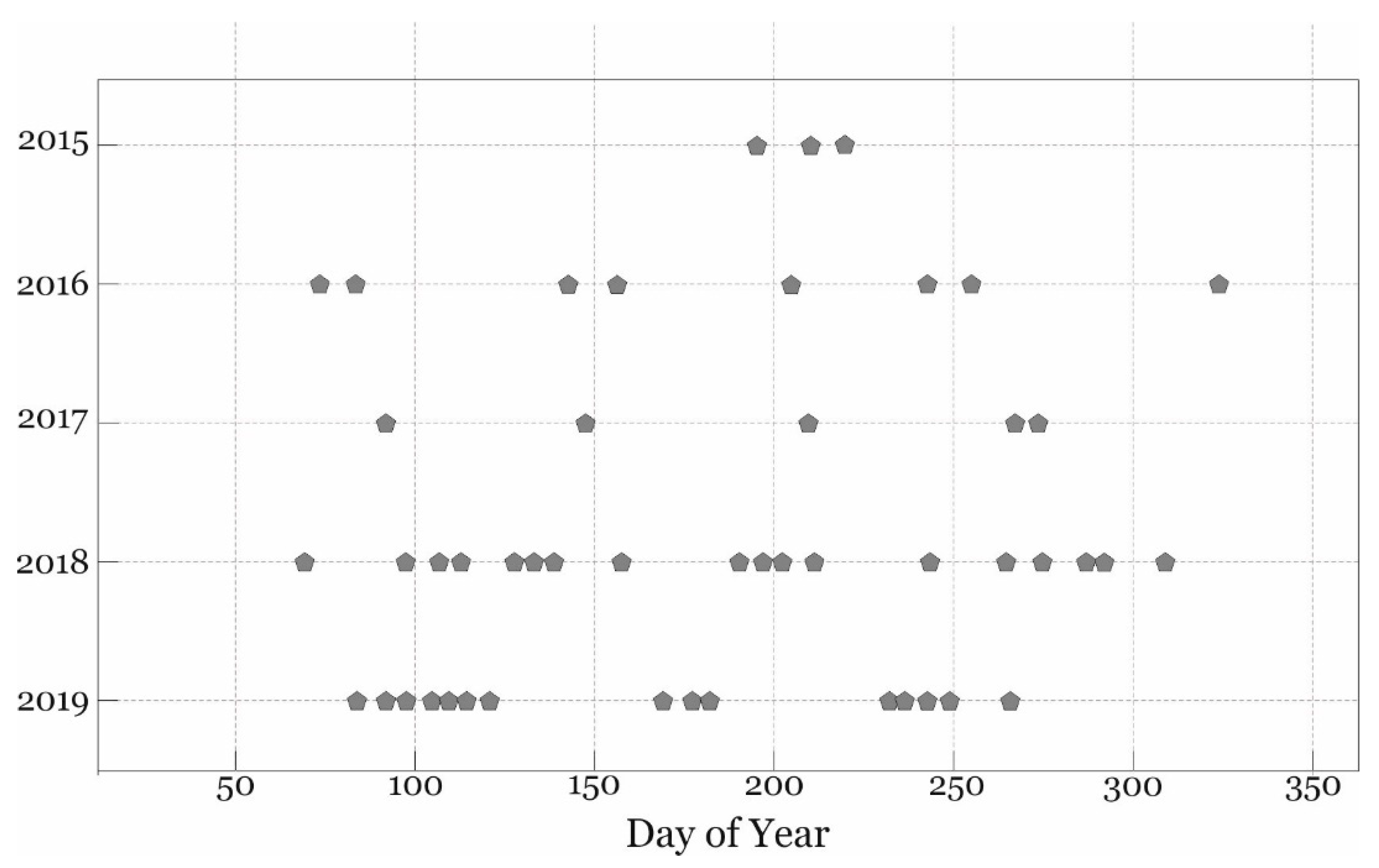
The Sentinel-2 imagery was downloaded from the Copernicus Open Access Hub repository using the sen2r package in R [54]. All of the available Sentinel-2 data from the years 2015–2019 (tile number: 33UXT), with a cloud cover below 10%, were downloaded and further processed, excluding winter imagery. In total, we used 49 images, acquired between 11 July 2015, and 23 September 2019 (Figure 2).

2.3. Methodology

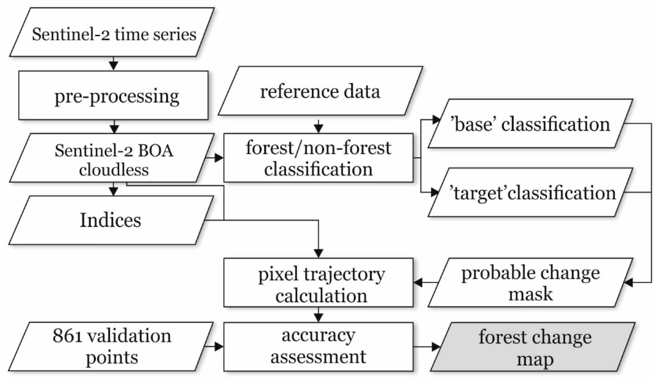
To achieve the objectives of the study, the following steps of analysis were performed: (i) The Sentinel-2 data were downloaded and pre-processed, including sen2cor correction, vegetation indices (VI) calculation, and cloud masking; (ii) “base” and “target” classifications were created, and their accuracy was assessed; based on these classifications, (iii) mask of probable change was generated; (iv) the spectral trajectories of the Sentinel-2 bands and indices were calculated for all the pixels in the area of probable change; (v) the accuracy of the detected changes was assessed using 861 validation points; and (vi) a forest change map was created, based on the highest accuracy change detection (Figure 3). All of the abovementioned steps were performed in R [55].

2.3.1. Data Pre-Processing

We downloaded all of the available Sentinel-2 imagery, with a cloud cover lower than 10%. For the imagery from after 2017, Bottom-of-Atmosphere (BOA) products were downloaded (if available), and for the older imagery, the sen2cor algorithm from the sen2r package was applied to transform the Top-of-Atmosphere (TOA) into BOA products. Then, four indices were calculated using s2_calcindices: NDMI, MSI, NBR, and TCW (Table 1). In the next step, we applied cloud masking to the Sentinel-2 BOA imagery and indices. The cloud mask was derived from the Sentinel Land Cover classification product (clouds, clouds shadows, and snow have been masked) [56]. The resulting products had a resolution of 10 m.

2.3.2. Classification and Probable Change Mask

Post-classification change is one of the most common methods of change detection, and it is simple and suitable for many applications. However, its accuracy is dependent on the accuracy of the input maps [22,57,58]. In some studies on forest disturbances, a forest mask was created for the beginning of the time series [59]. In our study, besides using this “base” forest map, we also created a “target” classification map for the end of the studied period. Both of the maps were classified into two classes: Coniferous forests (pine stands) and all other land cover types (broad-leaved forests, low vegetation, bare land, built-up areas, and water bodies). Reference samples for classification and validation were visually delineated for areas where no changes occurred during the studied period, and they include 112 polygons for conifer forest stands and 120 polygons for non-conifer forests (broad-leaved, water, agricultural, areas, and built-up). These reference polygons were randomly split into training and validation polygons in a 70:30 ratio. The base classification was calculated for the first available Sentinel-2 image for the study area, i.e., 11 July 2015. The target classification was calculated for the image from 31 August 2019. Based on the differences between the maps for 2015 and 2019, we produced the change map.
The classification was performed using the Random Forest (RF) algorithm, which is currently one of the most broadly-used classifiers in remote sensing land cover studies, mainly because of its ease of use and high accuracy [60]. Random Forest is an ensemble classifier that consists of a combination of decision trees [61]. The hyperparameters of the RF classifier consist of the number of trees that were set to 500 and a number of predictors at each split, which was tested from values of 1,2,3,5, and 10. The classification was performed using the superClass function from the RStoolbox package [62], and the rf classification algorithm from the randomForest package [63]. After the classification of single images, the accuracy assessment was performed using a validation dataset, and the achieved accuracies for both of the classifications exceeded 98% of the overall accuracy (Table 2).

2.3.3. Pixel Trajectory Assessment

For each pixel assigned to the probable change mask, we assessed the spectral trajectories, i.e., the values from the bands and indices for the whole studied period of time. In the case of spectral bands and TCW, the “raw’ values were used, while for NBR, NDMI and MSI indices the values were rescaled into the range from 0 to 1, which, based on tests, provided the best results regarding changes detection. To determine the date of a change (i.e., disturbance), we used the breakpoints function from the strucchange package [64]. This function computes the optimal breakpoints by minimizing the residual sum of squares in the regression model [65]. The parameters of the breakpoints function were set based on test runs, and the minimum length of a segment (h) was equal to two. Additionally, the confidence intervals for the model parameters in the breakpoints were calculated at a confidence level of 0.95, and we rejected breakpoints with intervals higher than 2. As the breakpoints function allow to detect multiple breaks, the first detected one was considered as a change in the forest. We tested breakpoints for reflectance values extracted from the visible red band (VIS R), red-edge bands (RE1, RE2, RE3), the near-infrared band (NIR), and two short-wave infrared (SWIR1, SWIR2) bands. Additionally, we tested four vegetation indices: NDMI, MSI, NBR, and TCW.

2.3.4. Accuracy Assessment and Forest Change Map

For the accuracy assessment of forest change maps we used the following measures of accuracy: An error matrix, an Overall Accuracy (OA), and the producer’s/user’s accuracies. Additionally, we calculated the macro-averaged F1 score, which is a harmonized mean of the producer’s and user’s accuracies [66]. To obtain reference samples, we used stratified random sampling, and 861 points were selected for accuracy assessment. Then, they were visually inspected based on the color and texture of the Sentinel-2 time series, and the date of the change (or no change class) was assigned to each of them. Finally, based on the highest accuracy change detection, forest change map was created, where each class represented the date of change (or no change).

3. Results

3.1. Map of Coniferous Forests and Probable Changes

The forest mask for 2015 covered approximately 158.2 km2, and that for 2019 covered approximately 158.4 km2. The potential change mask, where a change from coniferous forest to any non-coniferous class occurred, covered 4.95 km2, which equals 49,511 pixels (Figure 4). The increase of forest mask by 0.2 km2 indicates that the forest cover gain is also observed within the study area, and it is higher than forest cover loss. However, the main interest of this study was to analyze the areas where the loss of coniferous forests occurred.

3.2. Breakpoints Detection and Accuracy Assessment

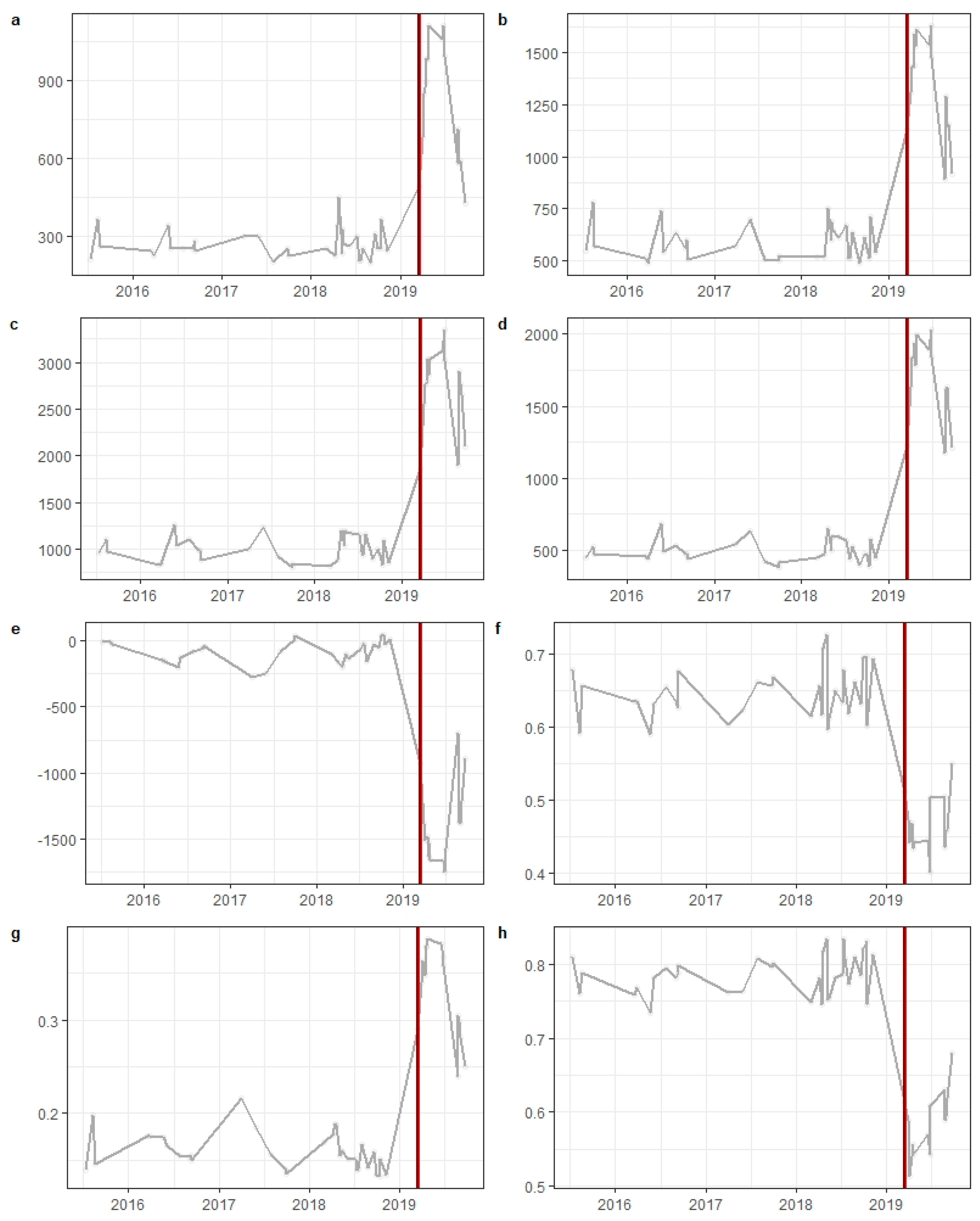
The changes in the coniferous forest stands caused an increase in the values in SWIR, RE1, VIS R bands, and MSI, and a decrease in NBR, TCW, and NDMI (Figure 5 and Figure 6).
The examples of pixel trajectories with both correctly and incorrectly detected breaks are shown in Figure 5 and Figure 6. In some cases, the breaks were detected after the actual break (Figure 5). There are clearly visible patterns of phenological trajectories of Scots pine stands (Figure 6); however, in most of the cases, they were not detected as breaks. The variations in reflectance and indices values are significantly larger after the change occurs.
The highest overall accuracy of forest change detection was obtained using the SWIR1 band (75.1% of OA; Table 3). SWIR1 was followed by RE1 (69.5% of OA) and SWIR2 (65.0% of OA). In general, single Sentinel-2 bands performed better than the vegetation indices. Among the indices, the best performance in detecting the changes was provided by the TCW (59% OA). Moderate accuracies above 60% of OA were also provided by the VIS R bands. The RE2, RE3, and NIR1 bands obtained very low accuracies (OA of 10% or below), and they were, thus not furthered analyzed.
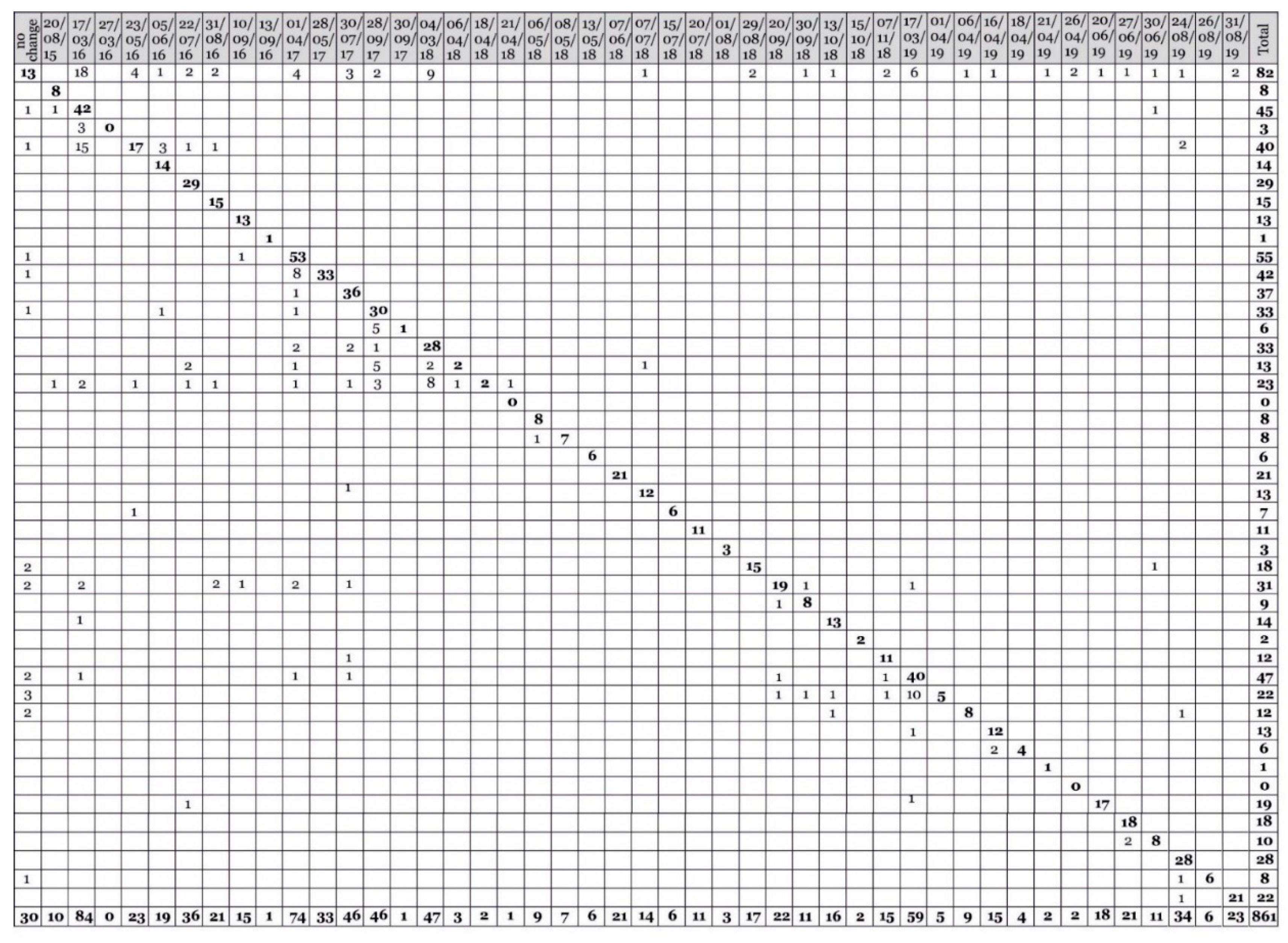
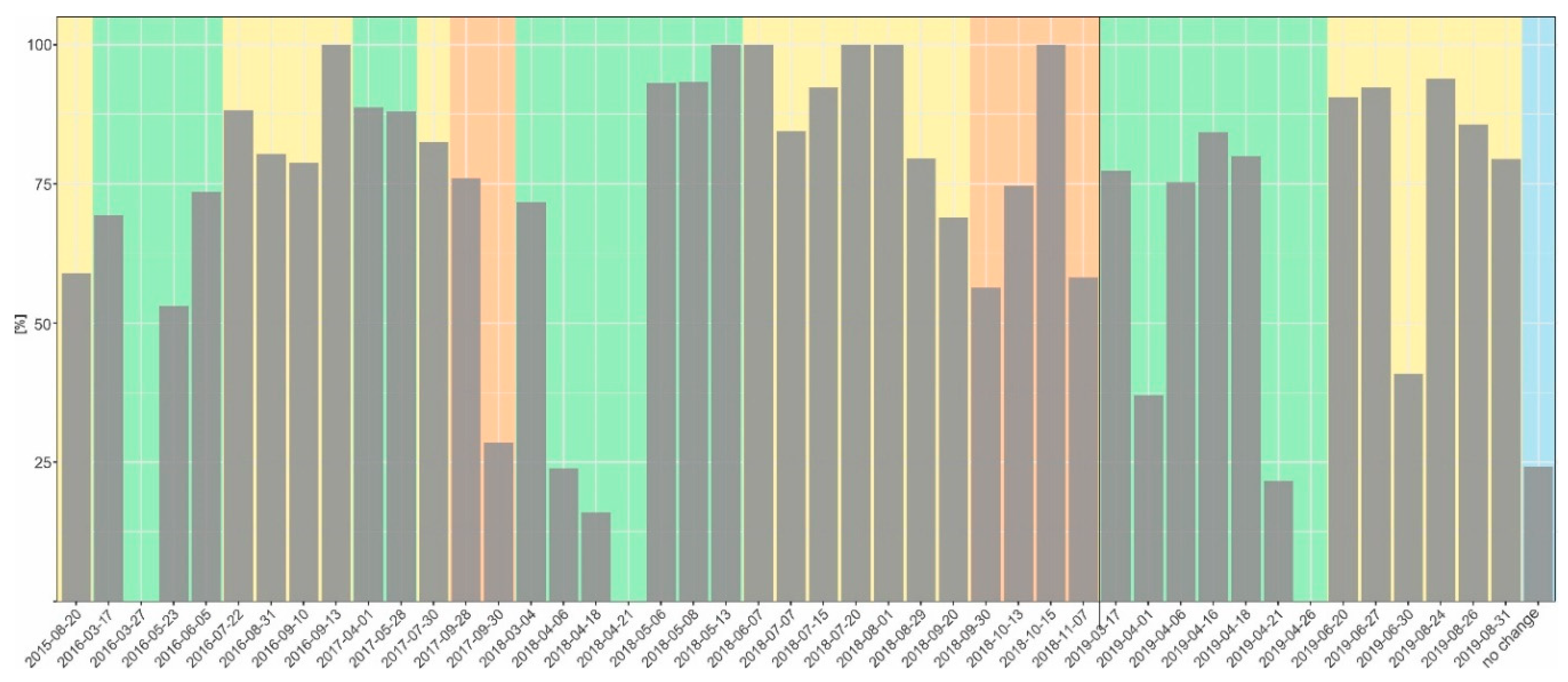
In the case of the best detection (SWIR1; Figure 7), the incorrectly detected pixels constituted 24.9% of all reference pixels. Among these misclassified pixels, 61.7% were detected after the actual break, 32.5% were not detected at all, and only 5.8% of all misclassified pixels were detected before the actual break. Furthermore, among the pixels detected after an actual change, 29% were detected within one date, and 50% within two dates after the actual change. Therefore, if also the neighboring detected dates were considered as positive detection, the overall accuracy increased to 80%. The assessment of temporal accuracy of the obtained forest change map, i.e., when the changes were detected with higher or lower accuracy, also showed some regularities (Figure 8). The lowest (zero or near-zero) macro-averaged F1 accuracies characterized early spring but, in all of the cases, not the first available spring date. Stable F1 accuracies generally characterized the summer months.

3.3. Forest Changes Map

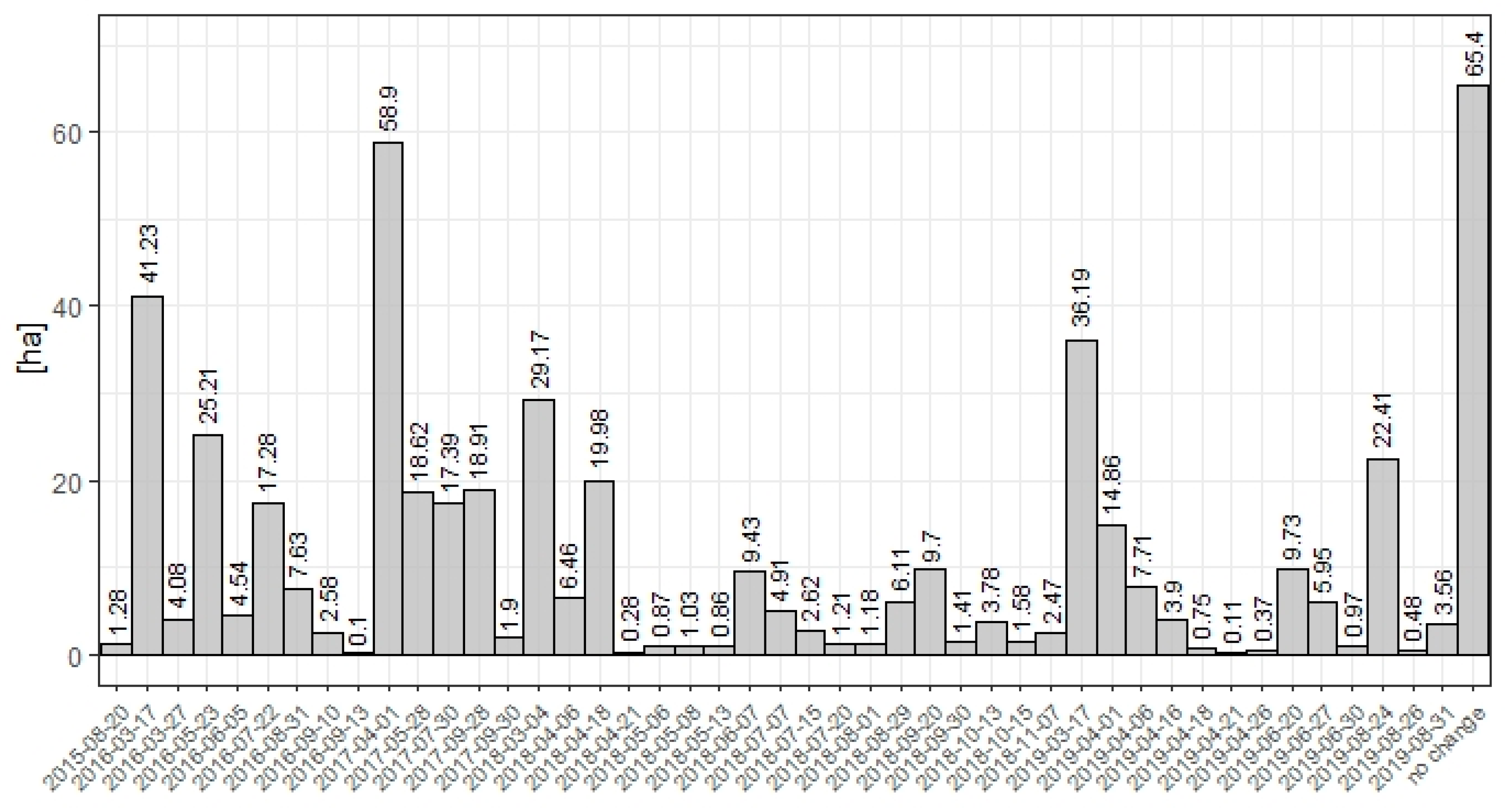
Based on the best detection in terms of accuracy (SWIR 1), we produced changes map in coniferous forest stands for the Milicz Forest District. Out of the 49,511 pixels, the breakpoints were detected for 42,971, which equals an area of the changes of 429.7 hectares (Figure 9). The most numerous changes were detected in the spring months, with the largest change area detected on 2017/04/01, which was equal to nearly 59 hectares, followed by that on 2016/03/17 (41 ha) and that on 2019/03/17 (36 ha). Regarding the annual changes in each examined year, starting from 2016, the changes exceeded 100 hectares, with the maximum area of the changes in 2017 equaling 115.7 hectares.
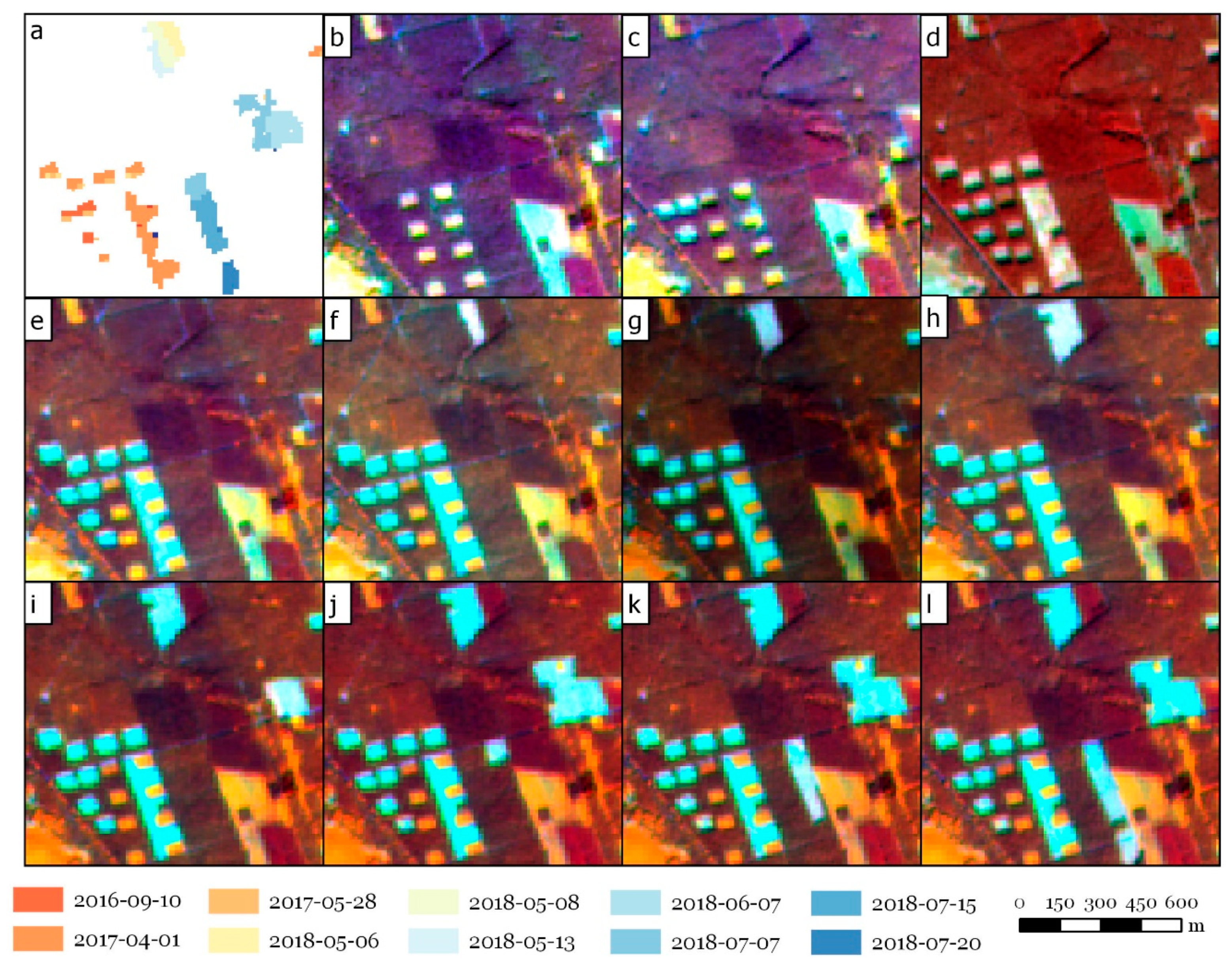
The obtained changes map allowed for the assessment of the spatial patterns and sizes of the coniferous forest changes (Figure 10). The area of the particular changes in coniferous forests varied from 100 m2 (i.e., a single Sentinel-2 pixel) to 29,100 m2. The largest forest changes were characterized by spatial homogeneity and regular shapes. In many cases, gradual changes were visible on consecutive dates.

4. Discussion

In this study, we developed a simple approach for detecting changes in Scots pine forest stands in the temperate zone using the Sentinel-2 dense time series. We determined pixel trajectories for the selected Sentinel-2 bands and vegetation indices for all the pixels assigned to the probable change mask between the years 2015 and 2019, with a total of 49,511 pixels (495 hectares). Our approach allowed for the detection of forest disturbances, with a satisfying accuracy of 75% of OA obtained for 46 classes (45 dates and one class representing no changes). We analyzed the sensitivity of different indices and Sentinel-2 bands in the detection of breaks. Interestingly, the indices commonly used in analyzing forest disturbances, such as NDMI or NBR, provided lower accuracies in change detection than the SWIR1 and RE1 Sentinel-2 bands.
Dense time series of Sentinel-2 imagery allows for continuous monitoring of forest ecosystems. We were able to detect Scots pine forest changes with the accuracy of 75%, and it increased to 80% if the neighboring detected dates were considered. Our results are in line with other studies on the Sentinel-2 time series in forest disturbances monitoring, which number, however, is still limited. In forest disturbance studies using the Sentinel-2 data, Puletti and Bascietto [49] used the NDVI series to separate cut from uncut forests, with high accuracy. The potential of the Sentinel-2 series was confirmed in the study of Navarro et al. [51] in the monitoring of cork oak decline. Puletti et al. [67] used Sentinel-2 time series to analyze the vegetation condition following extreme drought events and showed a reduction of trees photosynthetic activity.
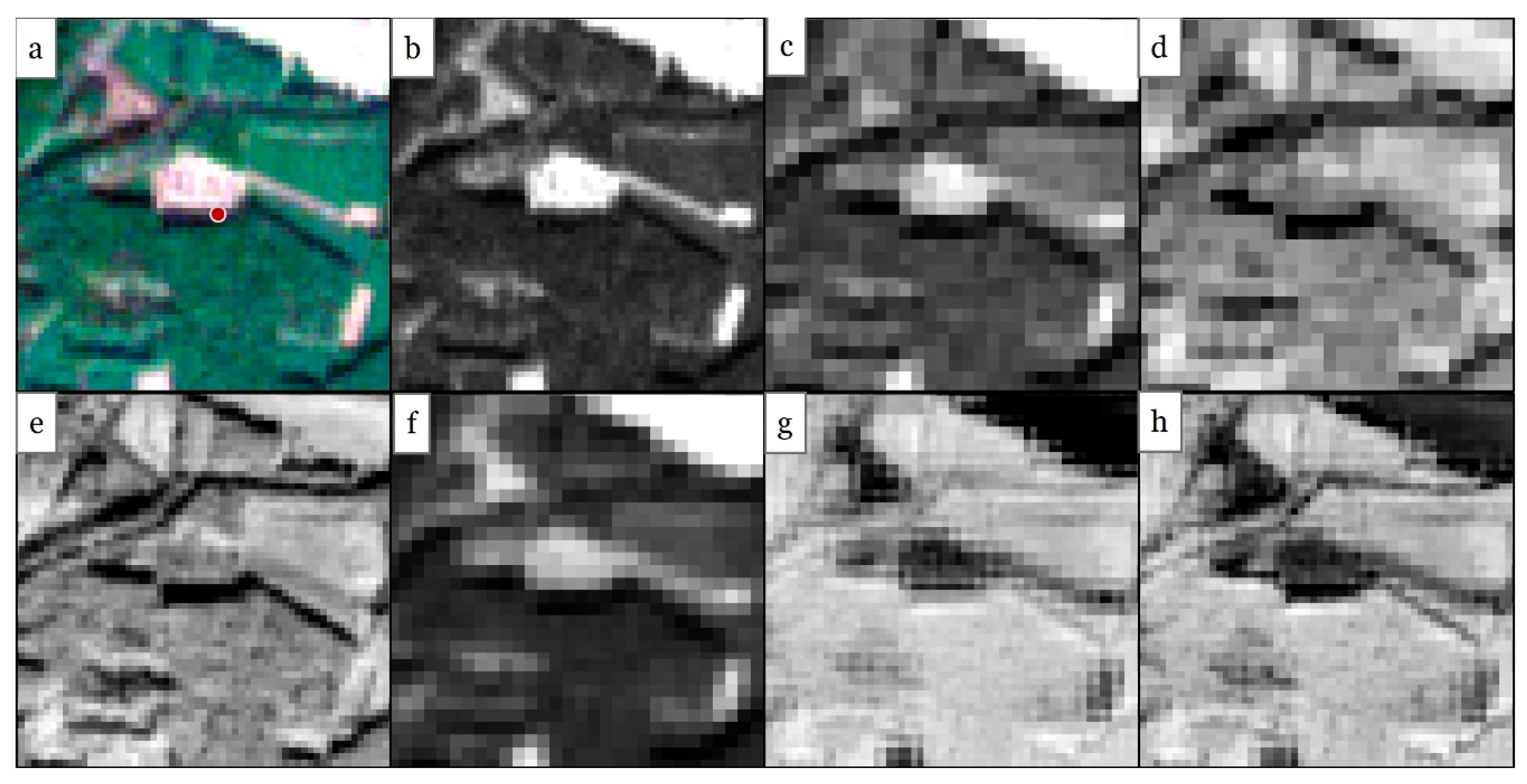
In our study, particularly the SWIR1 band performed effectively in detecting changes in Scots pine stands. This part of the spectrum is reported as a good indicator of vegetation water content [68] and is less impacted by soils and atmospheric noise [22]. Infested or dead trees have a significantly higher reflectance in SWIR than healthy ones at both the leaf and canopy level [30,51]. SWIR was also reported to be insensitive to internal shadows [39]. Schroeder et al. [69] reported that the SWIR part of the spectrum is the most effective in discriminating fires and clear-cuts. Sentinel-2, in comparison to other sensors, incorporates three red-edge spectral bands, which are highly sensitive to chlorophyll and nitrogen content and unaffected by structural properties [27,51]. In our study, the RE1 band provided high accuracy of 69% and, in contrast to RE2 and RE3, enabled the mapping of conifer forest changes. This significant difference in the performance of red-edge bands is due to very significant changes in this part of the spectrum as the wavelength increases (Figure 11). The red-edge part of the spectrum was also found to accurately retrieve green LAI and canopy chlorophyll content in the study of Delegido et al. [70]. The sensitivity of the red-edge region to the temporal dimension of the forest condition was reported by Zarco-Tejada et al. [26]. The study of Korhonen et al. [71] indicated a higher correlation between single bands, especially RE1, and the canopy cover and leaf area index than indices. Gitelson et al. [72] also reported the high sensitivity of reflectance, near 700 nm, to the chlorophyll concentration.
In other studies, where satellite imagery was used in forest disturbance mapping—mainly from Landsat missions—the indices were found to be an effective method. For example, the evaluation of bands and indices from the Landsat time series, based on a disturbance signal-to-noise metric, showed SWIR reflectance, and SWIR-based indices had the potential for disturbance detection [73]. SWIR-based indices—NDMI and NBR—were also found to be the most sensitive to forest changes among other vegetation indices, such as NDVI or EVI, in selective logging detection [39]. Hughes et al. [74] confirmed the potential of NDMI and NBR indices for forest change detection using the Landsat time series. In separating types of disturbance indices, utilizing SWIR bands was found to be of high importance in the study of Huo et al. [75]. Also, Abdullah et al. [30] confirmed that the Sentinel-2 based, red-edge- and SWIR-dependent indices had a high potential for detecting vegetation changes. In the study of Perbet et al. [76], Change Vector Analysis, based on the NIR, SWIR1, and VIS R bands, was performed in detecting deforestation due to their ability to discriminate forests from bare soil.
Different forest types and parameters may influence the performance of indices and bands in detecting changes. Additionally, different types of disturbances may have an impact on the performance of particular indices [39]. Among the four indices used in this study, the TCW performed better than the other indices in detecting changes. All of the examined indices, by definition, take advantage of the contrast between the SWIR and NIR parts of the spectrum. On the other hand, TCW, utilizes information also from other bands, including the SWIR2 and VIS R bands, which both performed moderately well in this study. Additionally, TCW has been reported to be insensitive to a topographically induced illumination angle [77].
According to our results, 429.7 hectares of coniferous stands were disturbed/deforested since 2015 in the studied area. Particularly in recent years, there is an increasing risk of drought in Poland as one of the effects of climate change. In Poland, a severe drought occurred in 2015 in almost all of the forests, particularly in Central and South-western Poland, where our study site is located [78]. A lack of sufficient amount of water available for the trees caused, among other things, a decrease in the health status of this area [78]. Currently, the climate change in temperate regions is related to higher temperatures, which increase tree water stress, cause physiological effects, and increase the tree vulnerability [3]. In central Europe, particularly conifer species, such as spruce and pine, are exposed to disturbances. Also, in other regions, e.g., in the Mediterranean basin, forests are exposed to drought effects [67]. However, there are different species- and site-specific aspects of growth responses to drought [79]. To evaluate the exact area of forests affected directly by drought, further studies in determining the types of disturbances should be carried out. In particular, planned clear cuts should be separated from disturbances caused by biotic and abiotic factors. Additionally, an explanation of the specific factors influencing the sensitivity to a particular change should be provided. As seen in Figure 10, the changes in forests are sometimes very rapid and occur within the months or even days. Therefore, the use of Sentinel-2, even taking into account the irregularity of acquisition, allows detecting forest disturbances with high temporal accuracy.
Many forest disturbances in temperate zones of Europe are small-scale, making the Sentinel-2 data a great tool for their detection. However, there are several sources of errors and uncertainties that should be considered in further studies. Firstly, there may be errors derived from the probable change mask due to errors in the base and target classifications. This is reported in many studies on change detection. Thus, these steps always have to be taken very carefully. Secondly, there are noises in the time series due to, e.g., undetected clouds or cloud shadows, as well as forest shadows. Forest shadows, which are very problematic in early spring and late autumn imagery, can result in errors, for example, changes detected at later dates. As seen in Figure 11, parts of the non-forested area covered by shadows are characterized by much lower values in single bands, although they are not so evident in the indices. The problem of object shadows is typically known in the processing of very-high-resolution imagery. Thus, the Sentinel-2 data with a 10- and 20-m resolution are now also sensitive to this issue. However, the indices are less sensitive to forest shadows. This problem might be solved in future studies by, for example, applying digital terrain models for shadow detection and then de-shadowing the problematic areas. Furthermore, frequent cloud cover results in the acquisition of irregular time series and sometimes missing data for the key periods of time. The Sentinel-2 time series used in this study are irregularly distributed over the studied years and growing seasons, which results from both the time of launching of Sentinel-2A and -2B missions and the atmospheric conditions, i.e., cloud cover. Thus, the date of the detection may not be an exact timing of the disturbance. This is partially a reason for the most numerous changes detected in the first spring dates, which in fact may also include of the changes from the winter period. Still, this information may be very useful for e.g., forest management, providing precise information where the change in forest stands occurred.
Another factor affecting errors in change detection is the misregistration of the Sentinel-2 imagery, which is visible as the geometric shifts for different acquisitions. In this study, there were several cases of false change detections on the border of forest/non-forest areas due to pixel shifts. Both the internal forest shadows and misregistration of the Sentinel-2 imagery may be reasons for the better performance of bands with a 20-m, rather than a 10-m resolution. The problem of misregistration was reported in other studies using the multi-temporal Sentinel-2 imagery [80]. Yan et al. [81] reported that, after applying a new processing baseline by ESA, the mean misregistration was about 0.4 of 10 m pixels.
The accuracy of the obtained forest change map results, in large part, from the abovementioned factors. Additionally, our approach has some limitations, i.e., it was tested on Scots pine stands, which have recently experienced a lot of disturbances. However, when analyzing broad-leaved forests, seasonal effects caused by phenology influence the result to a larger extent. Still, conifer species also exhibit some seasonal reflectance variations [82], which is seen in Figure 5 and Figure 6. Thus, they, in some cases, may also have an influence on the change detection algorithms.
In detecting forest changes, we used methods from the strucchange R package, designed to detect structural breaks [64]. As a change detection algorithm, it was used in the study of Hislop et al. on the Landsat time series [83], and it performed less accurately than LandTrendR. Also, Oeser et al. [59] used strucchange method to detect disturbance agents with high accuracy. In our study, it performed well and was easily applied to the Sentinel-2 time series. Therefore, it should be tested in other vegetation change studies using Sentinel-2.
While the definitions of forest disturbances differ, most disturbance events are related to the rapid removal or reduction of forest canopy [84]. Still, there are also subtle, non-stand replacements or gradual forest changes, such as thinning or stress damages. In comparison to abrupt changes in forest canopies and forest cover, these are more difficult to discriminate in terms of both their precise detection and the exact timing of their changes. Additionally, it might not be possible to detect changes covering, e.g., single trees, with the Sentinel-2 resolution. In our study, we focused mainly on stand replacement disturbances (i.e., forest stem removal) during this four-year time period. In the future, a longer time series of the Sentinel-2 imagery will be an invaluable source of information for forest and vegetation change analysis, so the automated methods of processing and detecting changes should be developed and used.

5. Conclusions

This study evaluated the use of the Sentinel-2 time series, consisting of 49 images from 2015 to 2019, in the detection of small-scale changes in coniferous forest stands. The comparison of selected Sentinel-2 bands and vegetation indices, based on an analysis of the breakpoints in pixels trajectories, showed varied usefulness in detecting forest disturbances. Surprisingly, the single Sentinel-2 SWIR1 and RE1 bands performed better than the analyzed vegetation indices, among which the Tasseled Cap Wetness provided the highest accuracy. However, the indices showed higher insensitivity to forest shadows. Given the high accuracy obtained with this simple approach, it might be useful in operational forest management to monitor forest changes.

Author Contributions

Conceptualization, E.G.; methodology, E.G.; validation, E.G.; formal analysis, E.G.; investigation, E.G.; data curation, E.G.; writing—original draft preparation, E.G., P.H. and J.S.; writing—review and editing, E.G. and P.H.; visualization, E.G.; funding acquisition, J.S. All authors have read and agreed to the published version of the manuscript.

Funding

This research was supported by the project I-MAESTRO. Project Innovative forest MAnagEment STrategies for a Resilient biOeconomy under climate change and disturbances (I-MAESTRO) is supported under the umbrella of ForestValue ERA-NET Cofund by the National Science Centre, Poland and French Ministry of Agriculture, Agrifood, and Forestry; French Ministry of Higher Education, Research and Innovation, German Federal Ministry of Food and Agriculture (BMEL) via Agency for Renewable Resources (FNR), Slovenian Ministry of Education, Science and Sport (MIZS). ForestValue has received funding from the European Union’s Horizon 2020 research and innovation programme under grant agreement N° 773324. The APC was funded by the Ministry of Science and Higher Education of the Republic of Poland for the University of Agriculture in Krakow for 2020.

Acknowledgments

We thank the anonymous reviewers for their valuable comments that helped improved the manuscript

Conflicts of Interest

The authors declare no conflict of interest.

References

  1. Lindner, M.; Maroschek, M.; Netherer, S.; Kremer, A.; Barbati, A.; Lexer, M.J.; Marchetti, M. Climate change impacts, adaptive capacity, and vulnerability of European forest ecosystems. For. Ecol. Manag. 2010, 259, 698–709. [Google Scholar] [CrossRef]
  2. Hartmann, H.; Moura, C.F.; Anderegg, W.R.L.; Ruehr, N.K.; Salmon, Y.; Allen, C.D.; Arndt, S.K.; Breshears, D.D.; Davi, H.; Galbraith, D.; et al. Research frontiers for improving our understanding of drought-induced tree and forest mortality. New Phytol. 2018, 218, 15–28. [Google Scholar] [CrossRef] [PubMed] [Green Version]
  3. Millar, C.I.; Stephenson, N.L. Temperate forest health in an era of emerging megadisturbance. Science 2015, 349, 823–826. [Google Scholar] [CrossRef] [PubMed]
  4. Plewa, R.; Mokrzycki, T. Występowanie, biologia i znaczenie gospodarcze kornika ostrozębnego Ips acuminatus (Gyllenhal, 1827) (Coleoptera, Curculionidae, Scolytinae) w Polsce. Sylwan 2017, 161, 619–629. [Google Scholar]
  5. Pastirčáková, K.; Adamčíková, K.; Pastirčák, M.; Zach, P.; Galko, J.; Kováč, M.; Laco, J. Two blue-stain fungi colonizing Scots pine (Pinus sylvestris) trees infested by bark beetles in Slovakia, Central Europe. Biologia (Bratisl.) 2018, 73, 1053–1066. [Google Scholar] [CrossRef]
  6. Siitonen, J. Ips acuminatus kills pines in southern Finland. Silva Fenn. 2014, 48, 1–7. [Google Scholar] [CrossRef] [Green Version]
  7. Grodzki, W.; Starzyk, J.R.; Kosibowicz, M. Impact of selected stand characteristics on the occurrence of the bark beetle Ips typographus (L.) in the Beskid Żywiecki Mountains. For. Res. Pap. 2014, 75, 159–169. [Google Scholar] [CrossRef] [Green Version]
  8. Grodzki, W. Forest decline in mountain spruce stands affected by bark beetle outbreaks in Poland. Attempt to spatial characteristic. In Proceedings of the Forest, Wildlife and Wood Sciences for Society Development, Prague, Czech Republic, 16–18 April 2009. [Google Scholar]
  9. Brzeziecki, B.; Hilszczański, J.; Kowalski, T.; Łakomy, P.; Małek, S.; Miścicki, S.; Modrzyński, J.; Sowa, J.; Starzyk, J.R. Problem masowego zamierania drzewostanów świerkowych w Leśnym Kompleksie Promocyjnym “Puszcza Białowieska”. Sylwan 2018, 162, 373–386. [Google Scholar]
  10. Jaime, L.; Batllori, E.; Margalef-Marrase, J.; Navarro, M.A.P.; Lloret, F. Scots pine (Pinus sylvestris L.) mortality is explained by the climatic suitability of both host tree and bark beetle populations. For. Ecol. Manag. 2019, 448, 119–129. [Google Scholar] [CrossRef]
  11. Davydenko, K.; Vasaitis, R.; Menkis, A. Fungi associated with Ips acuminatus (Coleoptera: Curculionidae) in Ukraine with a special emphasis on pathogenicity of ophiostomatoid species. Eur. J. Entomol. 2017, 114, 77–85. [Google Scholar] [CrossRef]
  12. Ploetz, R.C.; Hulcr, J.; Wingfield, M.J.; de Beer, Z.W. Destructive tree diseases associated with ambrosia and bark beetles: Black swan events in tree pathology? Plant Dis. 2013, 95. [Google Scholar] [CrossRef] [PubMed] [Green Version]
  13. Fernández-Fernández, M.; Naves, P.; Musolin, D.L.; Selikhovkin, A.V.; Cleary, M.; Chira, D.; Paraschiv, M.; Gordon, T.; Solla, A.; Papazova-Anakieva, I.; et al. Pine Pitch Canker and Insects: Regional Risks, Environmental Regulation, and Practical Management Options. Forests 2019, 10, 649. [Google Scholar] [CrossRef] [Green Version]
  14. Forests, S. Forests in Poland. 2017. Available online: http://www.lasy.gov.pl/pl/informacje/publikacje/in-english/forests-in-poland/lasy-w-polsce-2017-en.pdf/view (accessed on 20 February 2020).
  15. Durrant, T.H.; De Rigo, D.; Caudullo, G. Pinus Sylvestris in Europe: Distribution, Habitat, Usage and Threats. Available online: https://www.researchgate.net/profile/Giovanni_Caudullo/publication/299470777_Pinus_sylvestris_in_Europe_distribution_habitat_usage_and_threats/links/570b748508ae2eb942223b5c/Pinus-sylvestris-in-Europe-distribution-habitat-usage-and-threats.pdf (accessed on 20 February 2020).
  16. Hu, Y.; Dong, Y. Batunacun An automatic approach for land-change detection and land updates based on integrated NDVI timing analysis and the CVAPS method with GEE support. ISPRS J. Photogramm. Remote Sens. 2018, 146, 347–359. [Google Scholar] [CrossRef]
  17. Zarco-Tejada, P.J.; Hornero, A.; Beck, P.S.A.; Kattenborn, T.; Kempeneers, P.; Hernández-Clemente, R. Chlorophyll content estimation in an open-canopy conifer forest with Sentinel-2A and hyperspectral imagery in the context of forest decline. Remote Sens. Environ. 2019, 223, 320–335. [Google Scholar] [CrossRef]
  18. Kautz, M.; Meddens, A.J.H.; Hall, R.J.; Arneth, A. Biotic disturbances in Northern Hemisphere forests—A synthesis of recent data, uncertainties and implications for forest monitoring and modelling. Glob. Ecol. Biogeogr. 2017, 26, 533–552. [Google Scholar] [CrossRef]
  19. Meng, J.; Li, S.; Wang, W.; Liu, Q.; Xie, S.; Ma, W.; Ganguly, S.; Tucker, C.; Roy, S.; Thenkabail, P.S. Mapping Forest Health Using Spectral and Textural Information Extracted from SPOT-5 Satellite Images. Remote Sens. 2016, 8, 719. [Google Scholar] [CrossRef] [Green Version]
  20. Verbesselt, J.; Zeileis, A.; Herold, M. Near real-time disturbance detection using satellite image time series. Remote Sens. Environ. 2012, 123, 98–108. [Google Scholar] [CrossRef]
  21. Lausch, A.; Borg, E.; Bumberger, J.; Dietrich, P.; Heurich, M.; Huth, A.; Jung, A.; Klenke, R.; Knapp, S.; Mollenhauer, H.; et al. Understanding forest health with remote sensing, Part III: Requirements for a scalable multi-source forest health monitoring network based on data science approaches. Remote Sens. 2018, 10, 1120. [Google Scholar] [CrossRef] [Green Version]
  22. Banskota, A.; Kayastha, N.; Falkowski, M.J.; Wulder, M.A.; Froese, R.E.; White, J.C. Forest Monitoring Using Landsat Time Series Data: A Review. Can. J. Remote Sens. 2014, 40, 362–384. [Google Scholar] [CrossRef]
  23. Tao, X.; Huang, C.; Zhao, F.; Schleeweis, K.; Masek, J.; Liang, S. Mapping forest disturbance intensity in North and South Carolina using annual Landsat observations and field inventory data. Remote Sens. Environ. 2019, 221, 351–362. [Google Scholar] [CrossRef]
  24. Tang, X.; Bullock, E.L.; Olofsson, P.; Estel, S.; Woodcock, C.E. Near real-time monitoring of tropical forest disturbance: New algorithms and assessment framework. Remote Sens. Environ. 2019, 224, 202–218. [Google Scholar] [CrossRef]
  25. Hardisky, M.A.; Klemas, V.; Smart, R.M. The influence of soil salinity, growth form, and leaf moisture on the spectral radiance of Spartina alterniflora canopies. Photogramm. Eng. Remote Sens. 1983, 49, 77–83. [Google Scholar]
  26. Zarco-Tejada, P.J.; Hornero, A.; Hernández-Clemente, R.; Beck, P.S.A. Understanding the temporal dimension of the red-edge spectral region for forest decline detection using high-resolution hyperspectral and Sentinel-2a imagery. ISPRS J. Photogramm. Remote Sens. 2018, 137, 134–148. [Google Scholar] [CrossRef] [PubMed]
  27. Clevers, J.G.P.W.; Gitelson, A.A. Remote estimation of crop and grass chlorophyll and nitrogen content using red-edge bands on Sentinel-2 and -3. Int. J. Appl. Earth Obs. Geoinf. 2013, 23, 334–343. [Google Scholar] [CrossRef]
  28. Senf, C.; Seidl, R.; Hostert, P. Remote sensing of forest insect disturbances: Current state and future directions. Int. J. Appl. Earth Obs. Geoinf. 2017, 60, 49–60. [Google Scholar] [CrossRef] [Green Version]
  29. Hais, M.; Neudertová Hellebrandová, K.; Šrámek, V. Potential of Landsat spectral indices in regard to the detection of forest health changes due to drought effects. J. For. Sci. 2019, 65, 70–78. [Google Scholar] [CrossRef] [Green Version]
  30. Abdullah, H.; Skidmore, A.K.; Darvishzadeh, R.; Heurich, M. Sentinel-2 accurately maps green-attack stage of European spruce bark beetle (Ips typographus, L.) compared with Landsat-8. Remote Sens. Ecol. Conserv. 2019, 5, 87–106. [Google Scholar] [CrossRef] [Green Version]
  31. Hawryło, P.; Bednarz, B.; Wężyk, P.; Szostak, M. Estimating defoliation of Scots pine stands using machine learning methods and vegetation indices of Sentinel-2. Eur. J. Remote Sens. 2018, 51, 194–204. [Google Scholar] [CrossRef] [Green Version]
  32. Zhu, Z.; Woodcock, C.E.; Olofsson, P. Continuous monitoring of forest disturbance using all available Landsat imagery. Remote Sens. Environ. 2012, 122, 75–91. [Google Scholar] [CrossRef]
  33. Kennedy, R.E.; Yang, Z.; Cohen, W.B. Detecting trends in forest disturbance and recovery using yearly Landsat time series: 1. LandTrendr—Temporal segmentation algorithms. Remote Sens. Environ. 2010, 114, 2897–2910. [Google Scholar] [CrossRef]
  34. Cohen, W.B.; Yang, Z.; Kennedy, R. Detecting trends in forest disturbance and recovery using yearly Landsat time series: 2. TimeSync—Tools for calibration and validation. Remote Sens. Environ. 2010, 114, 2911–2924. [Google Scholar] [CrossRef]
  35. Pinheiro, T.F.; Escada, M.I.S.; Valeriano, D.M.; Hostert, P.; Gollnow, F.; Müller, H. Forest degradation associated with logging frontier expansion in the Amazon: The BR-163 region in southwestern pará, Brazil. Earth Interact. 2016, 20, 1–26. [Google Scholar] [CrossRef]
  36. Kupková, L.; Potůčková, M.; Lhotáková, Z.; Albrechtová, J. Forest cover and disturbance changes, and their driving forces: A case study in the Ore Mountains, Czechia, heavily affected by anthropogenic acidic pollution in the second half of the 20th century. Environ. Res. Lett. 2018, 13, 095008. [Google Scholar] [CrossRef]
  37. DeVries, B.; Verbesselt, J.; Kooistra, L.; Herold, M. Robust monitoring of small-scale forest disturbances in a tropical montane forest using Landsat time series. Remote Sens. Environ. 2015, 161, 107–121. [Google Scholar] [CrossRef]
  38. Brooks, E.B.; Wynne, R.H.; Thomas, V.A.; Blinn, C.E.; Coulston, J.W. On-the-fly massively multitemporal change detection using statistical quality control charts and landsat data. IEEE Trans. Geosci. Remote Sens. 2014, 52, 3316–3332. [Google Scholar] [CrossRef]
  39. Masiliūnas, D. Evaluating the Potential of Sentinel-2 and Landsat Image Time Series for Detecting Selective Logging in the Amazon; Wageningen University and Research Centre: Wageningen, The Netherlands, 2017. [Google Scholar]
  40. Hirschmugl, M.; Gallaun, H.; Dees, M.; Datta, P.; Deutscher, J.; Koutsias, N.; Schardt, M. Methods for Mapping Forest Disturbance and Degradation from Optical Earth Observation Data: A Review. Curr. For. Rep. 2017, 3, 32–45. [Google Scholar] [CrossRef] [Green Version]
  41. Hansen, M.C.; Roy, D.P.; Lindquist, E.; Adusei, B.; Justice, C.O.; Altstatt, A. A method for integrating MODIS and Landsat data for systematic monitoring of forest cover and change in the Congo Basin. Remote Sens. Environ. 2008, 112, 2495–2513. [Google Scholar] [CrossRef]
  42. de Almeida, C.A.; Coutinho, A.C.; dalla Mora Esquerdo, J.C.; Adami, M.; Venturieri, A.; Diniz, C.G.; Dessay, N.; Durieux, L.; Gomes, A.R. High spatial resolution land use and land cover mapping of the Brazilian legal Amazon in 2008 using Landsat-5/TM and MODIS data. Acta Amaz. 2016, 46, 291–302. [Google Scholar] [CrossRef]
  43. Coops, N.C.; Johnson, M.; Wulder, M.A.; White, J.C. Assessment of QuickBird high spatial resolution imagery to detect red attack damage due to mountain pine beetle infestation. Remote Sens. Environ. 2006, 103, 67–80. [Google Scholar] [CrossRef]
  44. Uddin, K.; Gilani, H.; Murthy, M.S.R.; Kotru, R.; Qamer, F.M. Forest Condition Monitoring Using Very-High-Resolution Satellite Imagery in a Remote Mountain Watershed in Nepal. Mt. Res. Dev. 2015, 35, 264–277. [Google Scholar] [CrossRef]
  45. Chehata, N.; Orny, C.; Boukir, S.; Guyon, D.; Wigneron, J.P. Object-based change detection in wind storm-damaged forest using high-resolution multispectral images. Int. J. Remote Sens. 2014, 35, 4758–4777. [Google Scholar] [CrossRef]
  46. Fassnacht, F.E.; Latifi, H.; Stereńczak, K.; Modzelewska, A.; Lefsky, M.; Waser, L.T.; Straub, C.; Ghosh, A. Review of studies on tree species classification from remotely sensed data. Remote Sens. Environ. 2016, 186, 64–87. [Google Scholar] [CrossRef]
  47. Zhu, Z.; Woodcock, C.E. Continuous change detection and classification of land cover using all available Landsat data. Remote Sens. Environ. 2014, 144, 152–171. [Google Scholar] [CrossRef] [Green Version]
  48. Jönsson, P.; Eklundh, L. TIMESAT—A program for analyzing time-series of satellite sensor data. Comput. Geosci. 2004, 30, 833–845. [Google Scholar] [CrossRef] [Green Version]
  49. Puletti, N.; Bascietto, M. Towards a Tool for Early Detection and Estimation of Forest Cuttings by Remotely Sensed Data. Land 2019, 8, 58. [Google Scholar] [CrossRef] [Green Version]
  50. Barton, I.; Király, G.; Czimber, K.; Hollaus, M.; Pfeifer, N. Treefall gap mapping using Sentinel-2 images. Forests 2017, 8, 426. [Google Scholar] [CrossRef] [Green Version]
  51. Navarro, A.; Catalao, J.; Calvao, J. Assessing the use of Sentinel-2 time series data for monitoring Cork Oak decline in Portugal. Remote Sens. 2019, 11, 2515. [Google Scholar] [CrossRef] [Green Version]
  52. Solon, J.; Borzyszkowski, J.; Bidłasik, M.; Richling, A.; Badora, K.; Balon, J.; Brzezińska-Wójcik, T. Physico-Geographical Mesoregions of Poland: Verification and Adjustment of Boundaries. Geogr. Pol. 2018, 91, 143–170. [Google Scholar] [CrossRef]
  53. Stereńczak, K.; Lisańczuk, M.; Parkitna, K.; Mitelsztedt, K.; Mroczek, P.; Miścicki, S. The influence of number and size of sample plots on modelling growing stock volume based on airborne laser scanning. Drewno 2018, 61. [Google Scholar] [CrossRef]
  54. Ranghetii, L.; Busetto, L. sen2r: An R Toolbox to Find, Download and Preprocess Sentinel-2 Data. R Package Version 1.0.2. Available online: https://sen2r.ranghetti.info (accessed on 20 February 2020).
  55. R Core Team. R: A Language and Environment for Statistical Computing; R Foundation for Statistical Computing: Vienna, Austria, 2019. [Google Scholar]
  56. Gatti, A.; Galoppo., A.C.; Castellani, C.; Carriero, F. Sentinel-2 Products Specification Document. Available online: https://sentinel.esa.int/documents/247904/685211/Sentinel-2-Products-Specification-Document (accessed on 20 February 2020).
  57. Tewkesbury, A.P.; Comber, A.J.; Tate, N.J.; Lamb, A.; Fisher, P.F. A critical synthesis of remotely sensed optical image change detection techniques. Remote Sens. Environ. 2015, 160, 1–14. [Google Scholar] [CrossRef] [Green Version]
  58. Liu, H.; Zhou, Q. Accuracy analysis of remote sensing change detection by rule-based rationality evaluation with post-classification comparison. Int. J. Remote Sens. 2004, 25, 1037–1050. [Google Scholar] [CrossRef]
  59. Oeser, J.; Pflugmacher, D.; Senf, C.; Heurich, M.; Hostert, P. Using intra-annual Landsat time series for attributing forest disturbance agents in Central Europe. Forests 2017, 8, 251. [Google Scholar] [CrossRef]
  60. Belgiu, M.; Drăgu, L. Random forest in remote sensing: A review of applications and future directions. ISPRS J. Photogramm. Remote Sens. 2016, 114, 24–31. [Google Scholar] [CrossRef]
  61. Breiman, L. Random forests. Mach. Learn. 2001, 45, 5–32. [Google Scholar] [CrossRef] [Green Version]
  62. Leutner, B.; Horning, N. Schwalb-Willmann RStoolbox: Tools for Remote Sensing Data Analysis. R Package Version 0.2.4. Available online: https://cran.r-project.org/package=RStoolbox (accessed on 20 February 2020).
  63. Liaw, a; Wiener, M. Classification and Regression by randomForest. R News 2002, 2, 18–22. [Google Scholar]
  64. Zeileis, A.; Leisch, F.; Homik, K.; Kleiber, C. strucchange: An R Package for Testing for Structural Change. J. Stat. Softw. 2002, 7, 1–38. [Google Scholar] [CrossRef] [Green Version]
  65. Zeileis, A.; Kleiber, C.; Walter, K.; Hornik, K. Testing and dating of structural changes in practice. Comput. Stat. Data Anal. 2003, 44, 109–123. [Google Scholar] [CrossRef] [Green Version]
  66. Zhong, L.; Hu, L.; Zhou, H. Deep learning based multi-temporal crop classification. Remote Sens. Environ. 2019, 221, 430–443. [Google Scholar] [CrossRef]
  67. Puletti, N.; Mattioli, W.; Bussotti, F.; Pollastrini, M. Monitoring the effects of extreme drought events on forest health by Sentinel-2 imagery. J. Appl. Remote Sens. 2019, 13, 1. [Google Scholar] [CrossRef]
  68. Olsen, J.L.; Ceccato, P.; Proud, S.R.; Fensholt, R.; Grippa, M.; Mougin, E.; Ardö, J.; Sandholt, I. Relation between seasonally detrended shortwave infrared reflectance data and land surface moisture in semi-arid Sahel. Remote Sens. 2013, 5, 2898–2927. [Google Scholar] [CrossRef] [Green Version]
  69. Schroeder, T.A.; Wulder, M.A.; Healey, S.P.; Moisen, G.G. Mapping wildfire and clearcut harvest disturbances in boreal forests with Landsat time series data. Remote Sens. Environ. 2011, 115, 1421–1433. [Google Scholar] [CrossRef]
  70. Delegido, J.; Verrelst, J.; Alonso, L.; Moreno, J. Evaluation of sentinel-2 red-edge bands for empirical estimation of green LAI and chlorophyll content. Sensors 2011, 11, 7063–7081. [Google Scholar] [CrossRef] [PubMed] [Green Version]
  71. Korhonen, L.; Hadi; Packalen, P.; Rautiainen, M. Comparison of Sentinel-2 and Landsat 8 in the estimation of boreal forest canopy cover and leaf area index. Remote Sens. Environ. 2017, 195, 259–274. [Google Scholar] [CrossRef]
  72. Gitelson, A.A.; Merzlyak, M.N.; Lichtenthaler, H.K. Detection of red edge position and chlorophyll content by reflectance measurements near 700 nm. J. Plant Physiol. 1996, 148, 501–508. [Google Scholar] [CrossRef]
  73. Cohen, W.B.; Yang, Z.; Healey, S.P.; Kennedy, R.E.; Gorelick, N. A LandTrendr multispectral ensemble for forest disturbance detection. Remote Sens. Environ. 2018, 205, 131–140. [Google Scholar] [CrossRef]
  74. Joseph Hughes, M.; Douglas Kaylor, S.; Hayes, D.J. Patch-based forest change detection from Landsat time series. Forests 2017, 8, 1–22. [Google Scholar]
  75. Huo, L.Z.; Boschetti, L.; Sparks, A.M. Object-based classification of forest disturbance types in the conterminous United States. Remote Sens. 2019, 11, 477. [Google Scholar] [CrossRef] [Green Version]
  76. Perbet, P.; Fortin, M.; Ville, A.; Béland, M. Near real-time deforestation detection in Malaysia and Indonesia using change vector analysis with three sensors. Int. J. Remote Sens. 2019, 40, 7439–7458. [Google Scholar] [CrossRef]
  77. Cohen, W.B.; Spies, T.A. Estimating structural attributes of Douglas-fir/western hemlock forest stands from landsat and SPOT imagery. Remote Sens. Environ. 1992, 41, 1–17. [Google Scholar] [CrossRef]
  78. Boczoń, A.; Kowalska, A.; Dudzińska, M.; Wróbel, M. Drought in Polish forests in 2015. Polish J. Environ. Stud. 2016, 25, 1857–1862. [Google Scholar] [CrossRef]
  79. Vanoni, M.; Bugmann, H.; Nötzli, M.; Bigler, C. Quantifying the effects of drought on abrupt growth decreases of major tree species in Switzerland. Ecol. Evol. 2016, 6, 3555–3570. [Google Scholar] [CrossRef] [PubMed]
  80. Lewinski, S.; Nowakowski, A.; Malinowski, R.; Rybicki, M.; Kukawska, E.; Krupiński, M. Aggregation of Sentinel-2 time series classifications as a solution for multitemporal analysis. Proc. SPIE 2017, 11. [Google Scholar] [CrossRef]
  81. Yan, L.; Roy, D.P.; Li, Z.; Zhang, H.K.; Huang, H. Sentinel-2A multi-temporal misregistration characterization and an orbit-based sub-pixel registration methodology. Remote Sens. Environ. 2018, 215, 495–506. [Google Scholar] [CrossRef]
  82. Rautiainen, M.; Lukeš, P.; Homolová, L.; Hovi, A.; Pisek, J.; Mõttus, M. Spectral properties of coniferous forests: A review of in situ and laboratory measurements. Remote Sens. 2018, 10, 207. [Google Scholar] [CrossRef] [Green Version]
  83. Hislop, S.; Jones, S.; Soto-Berelov, M.; Skidmore, A.; Haywood, A.; Nguyen, T.H. A fusion approach to forest disturbance mapping using time series ensemble techniques. Remote Sens. Environ. 2019, 221, 188–197. [Google Scholar] [CrossRef]
  84. Huang, C.; Goward, S.N.; Masek, J.G.; Thomas, N.; Zhu, Z.; Vogelmann, J.E. An automated approach for reconstructing recent forest disturbance history using dense Landsat time series stacks. Remote Sens. Environ. 2010, 114, 183–198. [Google Scholar] [CrossRef]
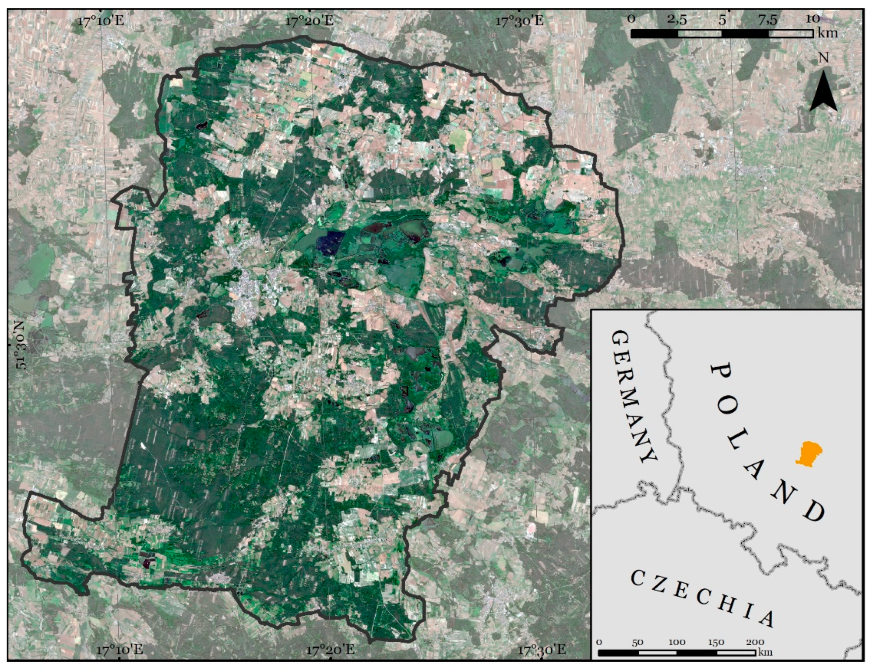
Figure 1. Study area of the Milicz Forest District located in south-western Poland. Sentinel-2 image from 30 June 2019, in natural band composition.
Remotesensing 12 01298 g001
Figure 2. Acquisition dates of the Sentinel-2 time series used in this study.
Remotesensing 12 01298 g002
Figure 3. Workflow used in this study.
Remotesensing 12 01298 g003
Figure 4. Coniferous forest cover changes in the years 2015–2019.
Remotesensing 12 01298 g004
Figure 5. The example of spectral trajectories for a selected pixel: red vertical lines—detected break dates, black vertical line—real change date.; (a) VIS R, (b) RE1, (c) SWIR1, (d) SWIR2, (e) TCW, (f) NDMI, (g) MSI, (h) NBR.
Remotesensing 12 01298 g005
Figure 6. The example of spectral trajectories for a selected pixel, where all bands and indices provided correct change date: red vertical lines—detected break dates, black vertical line—real change date.; (a) VIS R, (b) RE1, (c) SWIR1, (d) SWIR2, (e) TCW, (f) NDMI, (g) MSI, (h) NBR.
Remotesensing 12 01298 g006
Figure 7. Confusion matrix for the forest change map for the best breaks detection, i.e., SWIR1. Columns represent validation points, and rows represent forest change maps.
Remotesensing 12 01298 g007
Figure 8. Macro-averaged F1 score for the best detection map (SWIR1). Spring months highlighted in green, summer—yellow, autumn—orange.
Remotesensing 12 01298 g008
Figure 9. Changes detected in coniferous forests from 2015 to 2019.
Remotesensing 12 01298 g009
Figure 10. Part of the forest changes map based on pixel trajectory analysis (a) and selected Sentinel-2 time series: (b) 2016-07-22, (c) 2016-09-10, (d) 2017-04-01, (e) 2017-05-28, (f) 2018-05-06, (g) 2018-05-08, (h) 2018-05-13, (i) 2018-06-07, (j) 2018-07-07, (k) 2018-07-15, (l) 2018-07-20.
Remotesensing 12 01298 g010
Figure 11. Part of the Scots pine stands with deforestation example seen on image from 17 March 2016: (a) Sentinel-2 image in true color composition; (b) Red; (c) RE1; (d) RE2; (e) NIR1; (f) SWIR1; (g) TCW; (h) NDMI. The example pixel (red dot on true-color composition) was correctly detected using both indices but falsely detected using single bands as a change from 27 March, which was the consecutive date in the Sentinel-2 time series.
Remotesensing 12 01298 g011
Table 1. Indices used in the study (NIR—Near Infrared, SWIR—Short wave infrared, VIS B—visible blue, VIS G—visible green, VIS R—visible red).
IndexEquation
Normalized Difference Moisture Index (NDMI) N I R 1 S W I R 1 N I R 1 + S W I R 1
Moisture Stress Index (MSI) S W I R 1 N I R 1
Normalized Burn Ratio (NBR) N I R 1 S W I R 2 N I R 1 + S W I R 2
Tasseled Cap Wetness (TCW) 0.1509 × V I S   B + 0.1973 × V I S   G + 0.3279 × V I S   R + 0.3406 × N I R 1 0.7112 × S W I R 1 0.4572 × S W I R 2
Table 2. Accuracy assessment of coniferous forest classification for 2015 and 2019. The number in the confusion matrix represents the number of pixels in the validation dataset.
Coniferous ForestOther Classes
2015Coniferous forest101224
Other classes5995
Producer’s Accuracy99.5197.64
User’s Accuracy97.6999.50
2019Coniferous forest101619
Other classes1995
Producer’s Accuracy99.9098.13
User’s Accuracy98.1699.90
Table 3. Accuracy assessment of break dates (changes) detected using selected variables.
Input OA
SWIR175.1
RE1 69.5
SWIR 2 65.0
VIS R 62.5
TCW59.0
MSI 49.2
NDMI 46.6
NBR 53.1