Potato Late Blight Detection at the Leaf and Canopy Levels Based in the Red and Red-Edge Spectral Regions

Abstract

Potato late blight, caused by Phytophthora infestans, is a major disease worldwide that has a significant economic impact on potato crops, and remote sensing might help to detect the disease in early stages. This study aims to determine changes induced by potato late blight in two parameters of the red and red-edge spectral regions: the red-well point (RWP) and the red-edge point (REP) as a function of the number of days post-inoculation (DPI) at the leaf and canopy levels. The RWP or REP variations were modelled using linear or exponential regression models as a function of the DPI. A Support Vector Machine (SVM) algorithm was used to classify healthy and infected leaves or plants using either the RWP or REP wavelength as well as the reflectances at 668, 705, 717 and 740 nm. Higher variations in the RWP and REP wavelengths were observed for the infected leaves compared to healthy leaves. The linear and exponential models resulted in higher adjusted R² for the infected case than for the healthy case. The SVM classifier applied to the reflectance of the red and red-edge bands of the Micasense^® Dual-X camera was able to sort healthy and infected cases with both the leaf and canopy measurements, reaching an overall classification accuracy of 89.33% at 3 DPI when symptoms were visible for the first time with the leaf measurements and of 89.06% at 5 DPI, i.e., two days after the symptoms became apparent, with the canopy measurements. The study shows that RWP and REP at leaf and canopy levels allow detecting potato late blight, but these parameters are less efficient to sort healthy and infected leaves or plants than the reflectance at 668, 705, 717 and 740 nm. Future research should consider larger samples, other cultivars and the test of unmanned aerial vehicle (UAV) imagery for field-based detection.

1. Introduction

Potato late blight, caused by Phytophthora infestans, is a significant disease worldwide that has a significant economic impact on potato crops, which is estimated to be over US$5.45 million per year. Such impact is due to the capacity of the agent to destroy the plants and tubers rapidly and to propagate to large areas during the growing season thanks to the production of secondary inoculum [1,2]. There is, therefore, the need to detect the disease for avoiding its rapid propagation [3]. Field scouting and continuous preventive pesticide applications have been adopted to prevent yield losses, but these strategies are either time-consuming or expensive, and they are not environmentally friendly. An alternative is to use imagery having the appropriate temporal and spatial scale to detect the disease at early stages by sensing the changes in chemical and physical properties of the crop [4]. Indeed, late blight causes chlorosis that can be detected in the visible region of the spectra (400 to 700 nm) [5]. The disease can also change the leaf structure, which is detectable in the near-infrared spectral region (700 to 1300 nm) [6,7].

One particular spectral region in the visible domain is the red region, which corresponds to one of the two chlorophyll absorption bands [8]. Another spectra domain is the red-edge region, a transition zone from the red to the near-infrared region, which is usually located between 660 to 780 nm [9]. Such a transition zone is due to the maximal chlorophyll absorbance in the red wavelength and the high reflectance in the near-infrared wavelengths because of multiple scatterings of the near-infrared radiation by the leaf mesophyll [10]. According to Pu et al. [11], two optical parameters related to the red-edge region can be defined: the red-well position (RWP or R0) and the red-edge inflection point (REP). RWP is the wavelength in the red region between 660 and 680 nm that corresponds to the minimum reflectance because of maximum chlorophyll absorption. REP is the wavelength corresponding to the inflection point of the spectral curve between the red and near-infrared spectral domains. At this wavelength, the reflectance slope in the red-edge region is maximal [12]. Changes in the RWP and REP can be related to the presence of potato late blight. Indeed, this disease is caused by a hemibiotrophic pathogen that affects the leaf chemical composition, specifically its chlorophyll content, and induces changes in the internal leaf structure that can be detected using the near-infrared reflectance [13,14]. Shifts of the REP to longer or shorter wavelengths have already been related to changes in the chemical and morphological plant status [15].

In the literature, there are several studies that related band reflectances or vegetation indices to late blight occurrence in potato or tomato crops [16,17,18,19,20,21,22], but none of them tested the use of RWP and REP to detect the disease. All of them but Fernández et al. [21] and Gold et al. [22] were based on one or two dates of experimentations without reporting the moment of inoculation, and thus they were not able to determine the time after inoculation when the disease could be detected with spectral information. This study aims to improve the understanding of the spectral changes of RWP and REP at the leaf and canopy levels due to late blight disease on potato plants from the moment of inoculation. In particular, we modeled the changes in RWP and REP at the leaf and canopy levels as a function of the days post-inoculation (DPI). We also developed a Support Vector Machine (SVM) algorithm [23] to sort healthy and infected leaves or plants by using two types of input features: i) the wavelengths corresponding to RWP or REP; and (ii) the reflectances of the red and red-edge bands of the Micasense^® Dual-X camera (Micasense, Inc., Seattle, WA, USA). The results of this study will be used to test UAV images acquired with this camera for detecting late blight disease over potato fields.

2. Materials and Methods

2.1. Experiment

The study used data that were acquired as part of the experiment, which is detailed in Fernández et al. [21]. We will here summarize the main steps of the experiment. The experiment used two groups (healthy and infected) of eight Shepody potato plants grown in a walk-in growth chamber located at the Biotron facilities of the University of Western Ontario (London, ON, Canada). The chamber has a constant relative humidity of 65%, a photoperiod of 12 h at 23 °C, followed by a dark period of 12 h at 18 °C. The infected plants were inoculated by spraying at the flowering phenological stage 200 µL of a sporangia suspension of Phytophthora infestans at the concentration of 1 × 10⁵ sporangia mL⁻¹ on marked primary leaflets. A total of 101 leaflets were inoculated. To follow the spectral changes of each leaflet by acquiring spectra over the same leaflets, we marked the healthy and inoculated leaflets at the base of the petiole with a small piece of white tape which was numbered. Control (healthy) and infected leaflets were chosen from the middle and the top of the canopy so that they were larger than the leaf clip measurement area to avoid low reflectance measurements when the leaves were too small [21]. Healthy plants were placed in a separate chamber to avoid cross-contamination.

Radiances between 350 and 2500 nm at 1.4 nm sampling intervals with a 25° field of view (FOV) bare fiber optic cable were measured at the leaf and canopy levels three hours before inoculation, until six days post-inoculation (DPI), with an ASD FieldSpec PRO FR spectroradiometer (ASD Inc., Boulder, CO, USA). Both the leaf and canopy spectra were acquired and calibrated using the RS3 version 6.4 software from ASD (ASD Inc., Boulder, CO, USA). The leaf-level reflectance spectra were acquired at the center of the marked leaflets of healthy and infected plants using a leaf clip, with a white Goretex (99% reflectance) and a black reference, attached to an ASD high-intensity probe equipped with a light source and a fiber optic cable. For each experiment day, we acquired a total of 101 spectra over the infected leaves and 124 spectra over the healthy leaves.

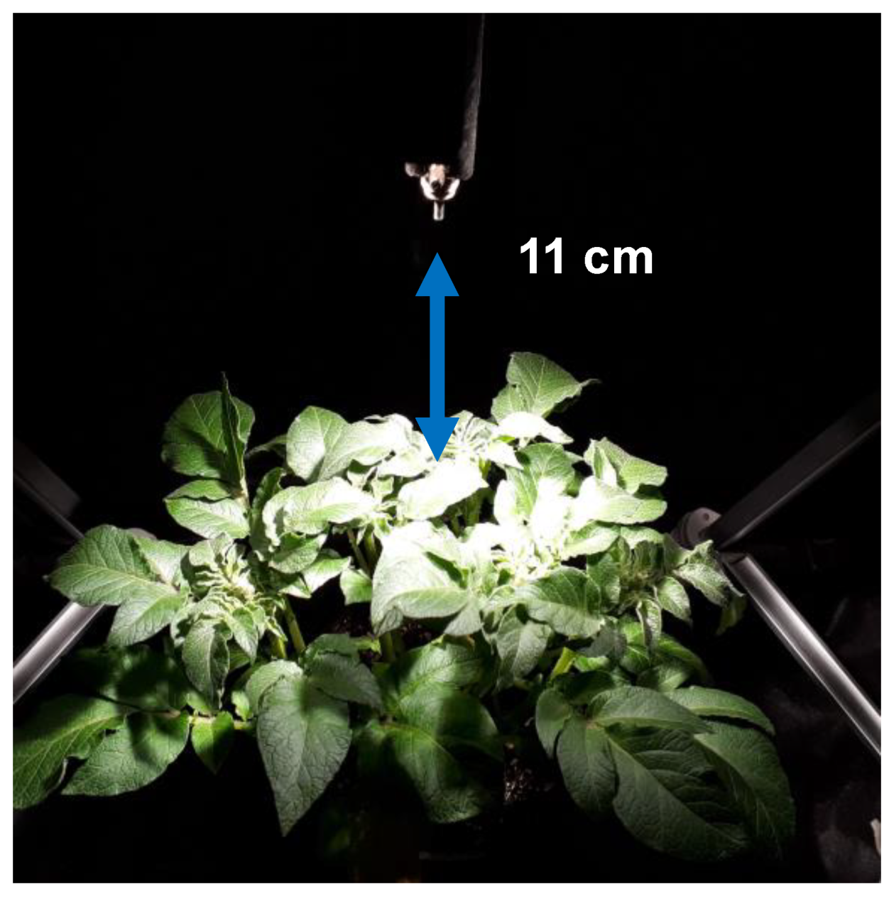
The canopy-level spectra were acquired on each plant by placing the 25° FOV bare fiber optic cable at 11 cm from the top of the canopy (Figure 1). Plants were illuminated with two ASD halogen lamps (ASD Inc., Boulder, CO, USA), each of them angled at 45° from the horizontal line and located on each side of the plant. Canopy spectra were acquired over eight healthy and eight infected plants at each day of the experiment. For each plant, the canopy reflectance was measured four times after rotating the plant 90°. This allowed obtaining a total of 32 healthy and 32 infected canopy reflectance spectra at each day of the experiment. The measured plant area was 82.83 cm² according to Equation (1) as reported by Fernández et al. [21]:

A(cm²) = π * (tan FOV * h)²

(1)

where

• A = Measured plant area at the top of the plant canopy (in cm²);
• FOV = field of view angle of the optic fiber (= 25°);
• h = distance between the top of the canopy and the fiber optic sensor (= 11 cm).

2.2. Methodology

All data were processed using MATLAB R2019a (MathWorks, Inc., Natick, MA, USA). The spectra collected at the leaf and canopy levels from the healthy and infected plants were first cropped to the 400 to 900 nm range. Secondly, the raw spectra were converted to reflectance spectra using the ViewSpec Pro version 6.2.0 software (ASD Inc., Boulder, CO, USA). These reflectance spectra were then subjected to a Savitzky–Golay [24] filtering method to reduce instrumental noise and to a multiplicative scatter correction (MSC) to remove additive and multiplicative scattering [25]. The filtered reflectance spectra were used to compute the first-order derivative (FD) of the reflectance spectra that represents the signal change between two adjacent wavelengths [26]. The FD is computed as follows [27]:

FD (λ) = [R (λ + Δλ) − R (λ − Δλ)]/2Δλ

(2)

where

• FD (λ) = first-order derivative of the reflectance spectrum at wavelength λ;
• R = reflectance at specified wavelengths λ + Δλ; or λ − Δλ;
• λ = wavelength of the spectrum (nm);
• Δλ; = difference between two successive wavelengths, i.e., 1.4 nm.

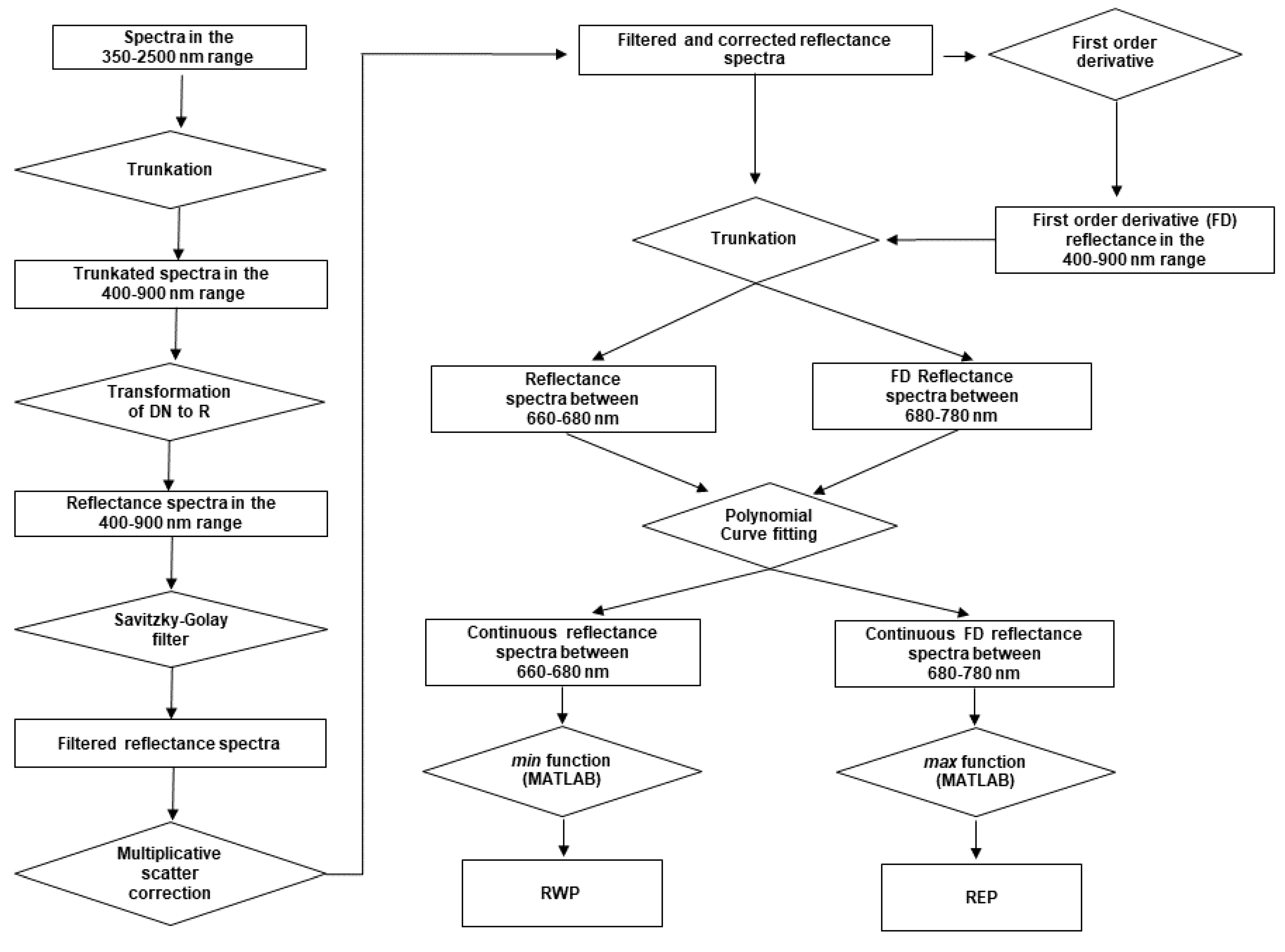
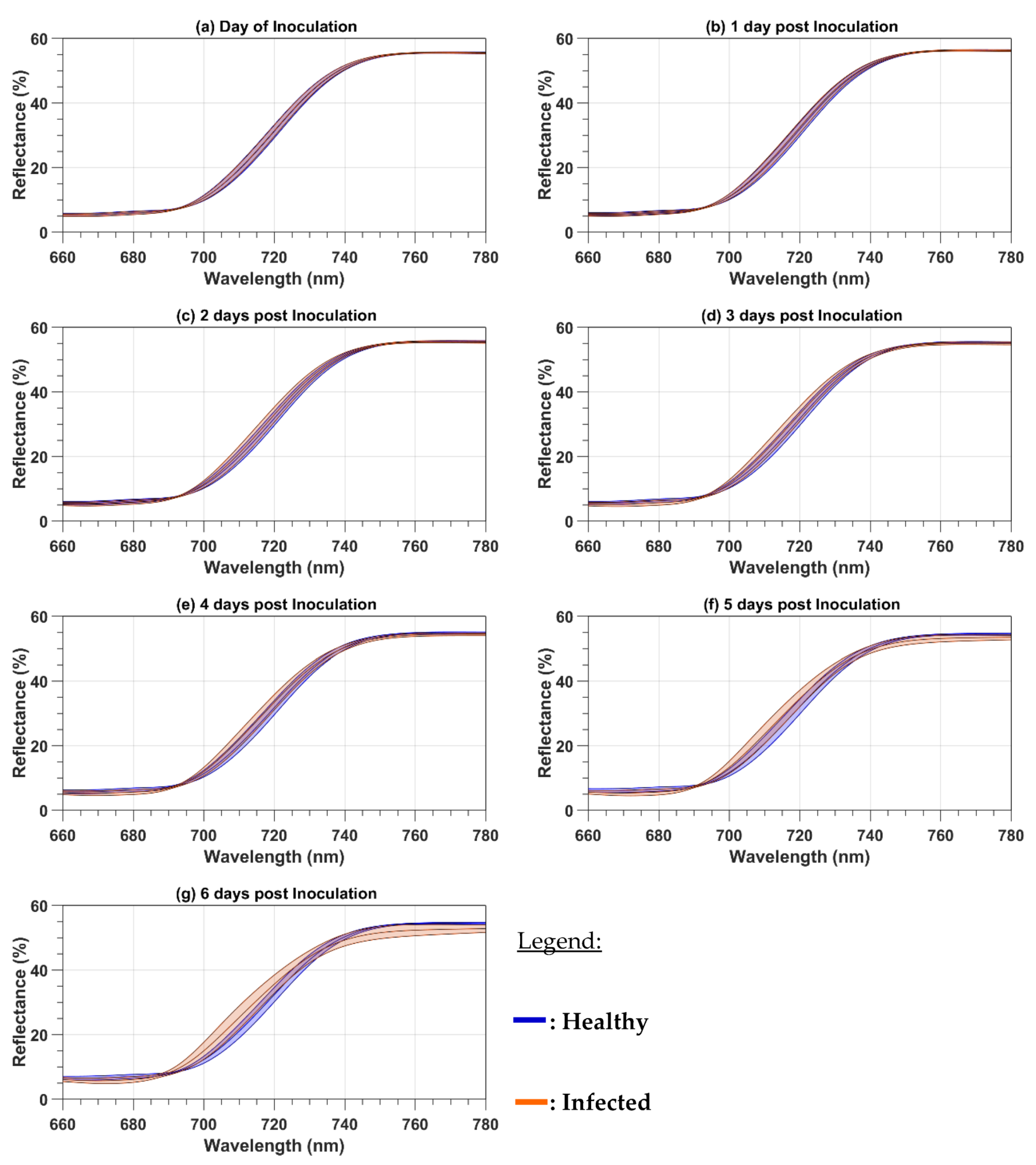
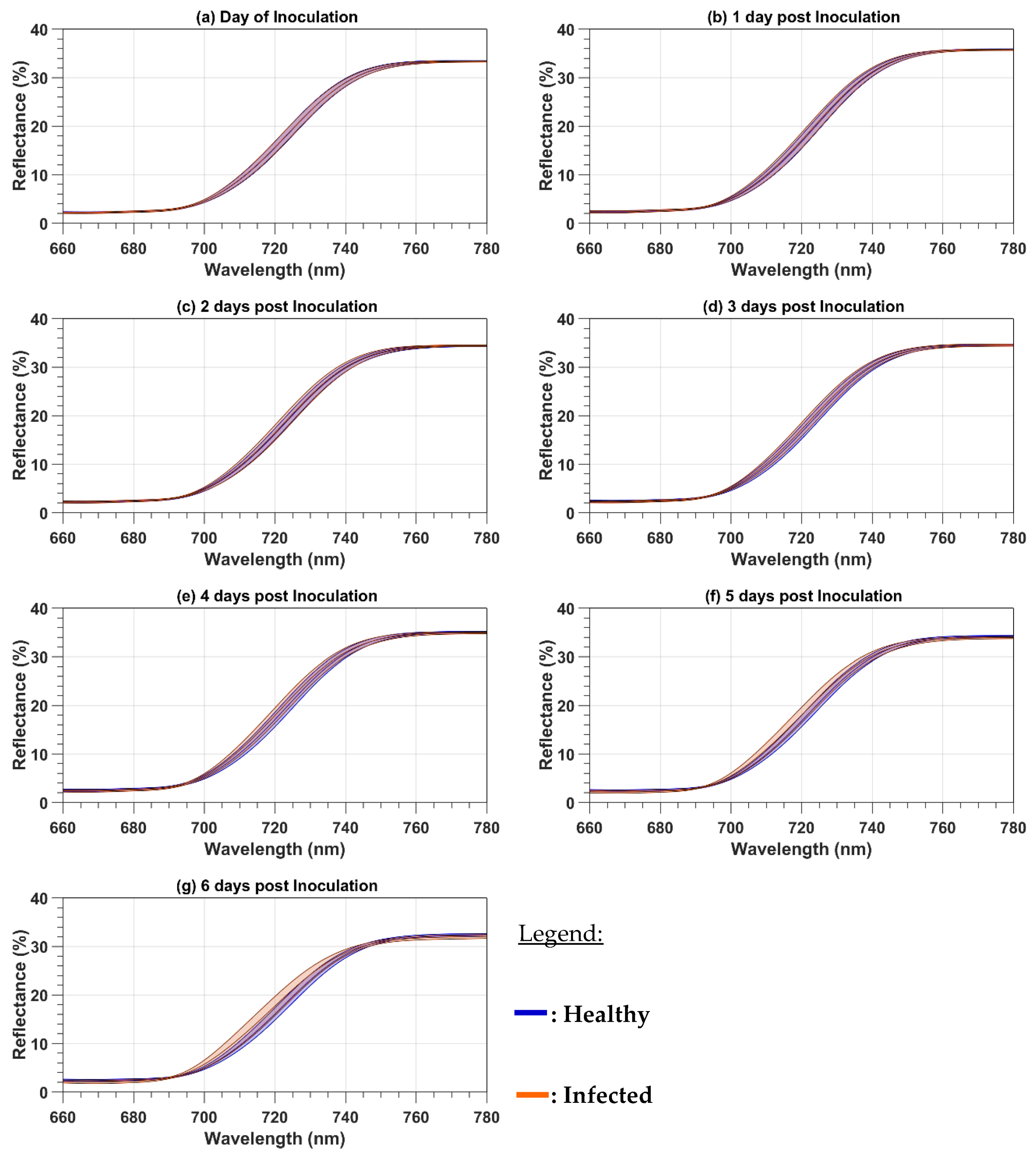
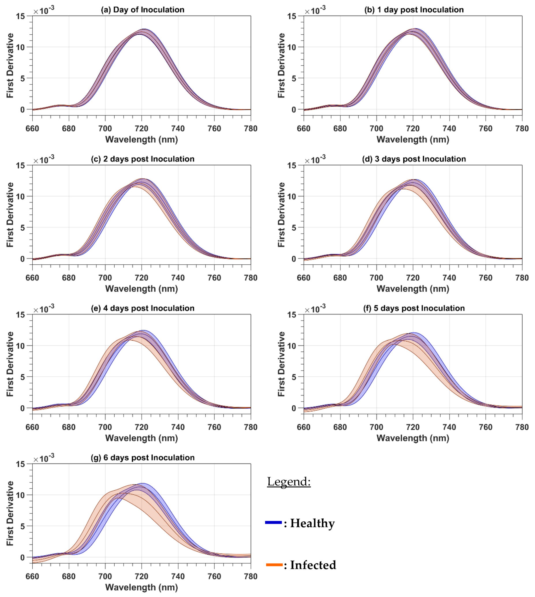
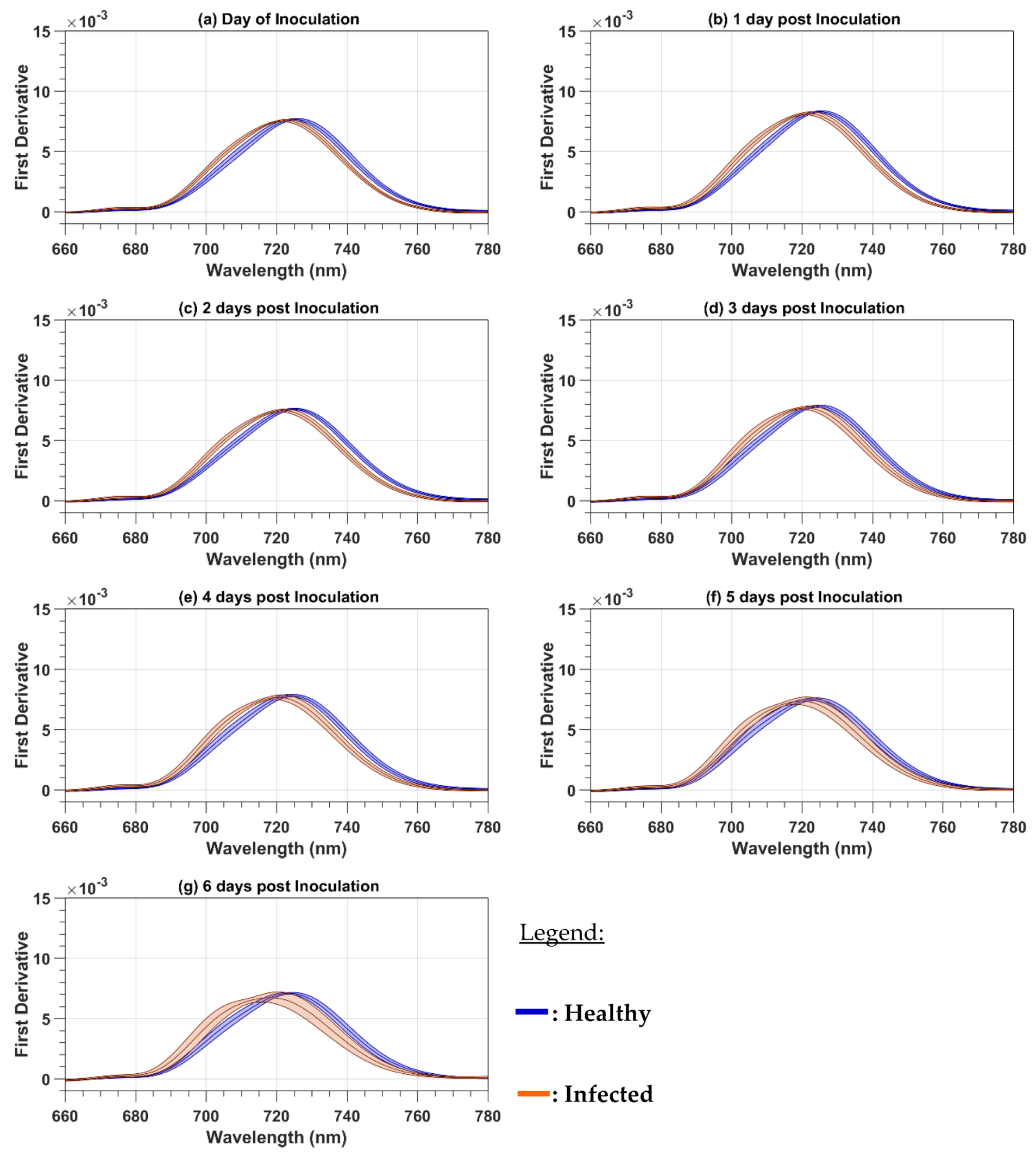
Because the paper focuses on the red and red-edge regions, both the reflectance and the first-order derivative spectra were cropped to the 660 to 780 nm spectral range. The mean cropped spectra were plotted to observe the spectral variations as a function of the DPI. The mean reflectance spectra were calculated as a simple average of all 124 (101) healthy (infected) leaf spectra and all the 32 healthy or infected canopy spectra. With the spectra acquired on both the leaf and canopy levels, two spectral parameters were computed for every day of evaluation from 0 to 6 DPI. The first one is the red-well point (RWP), which corresponds to the wavelengths having the minimum reflectance value in the red region [11]. The methodology to compute the RWP involved three steps (Figure 2). First, the reflectances in the red region, i.e., between 660 and 680 nm, of each spectrum were selected. Second, a curve was fitted to the reflectance values to make them continuous. Finally, since the RWP is the wavelength corresponding to the minimum reflectance value, it was determined by applying the min function of MATLAB R2019a (MathWorks, Inc., Natick, MA, USA) to the fitted curve to retrieve the minimum reflectance and then the corresponding wavelength. The second parameter is the red-edge point (REP), which is the wavelength of the inflection point of the reflectance spectra in the red-edge region, i.e., between 680 and 780 nm [28]. REP is, therefore, the wavelength corresponding to the maximum value of the FD spectra. This value was determined as follows (Figure 2). First, the FD spectra were truncated to the red-edge region, and a curve was fitted over this spectral range to make the FD data continuous. The maximum of the fitted curve was then determined by using the max function of MATLAB R2019a. For both REP and RWP, the curve has a parabolic shape that is modeled using a second-order polynomial function.

With the computed RWP and REP wavelengths for each DPI, a t-test means comparison was used to analyze the difference of the RWP and REP values between healthy and infected cases as a function of the DPI. A t-test mean comparison usually assumes that the data have a normal distribution and that the variance is equal, but Posten (1984) [29] showed that such a t-test is highly robust to deviations from the normality assumption. The normality assumption for the RWP and REP data distribution was visually assessed through histograms graphed with both the leaf- and canopy-level values. The equal variance assumption was tested with a two-sample F-test (vartest2 function of MATLAB R2019a), which returned an acceptance of the null hypothesis. The t-test was computed using RWP and REP values from 124 and 101 healthy and infected leaves. At the canopy level, the t-test was computed using for RWP and REP data from 32 healthy and 32 infected spectral measurements.

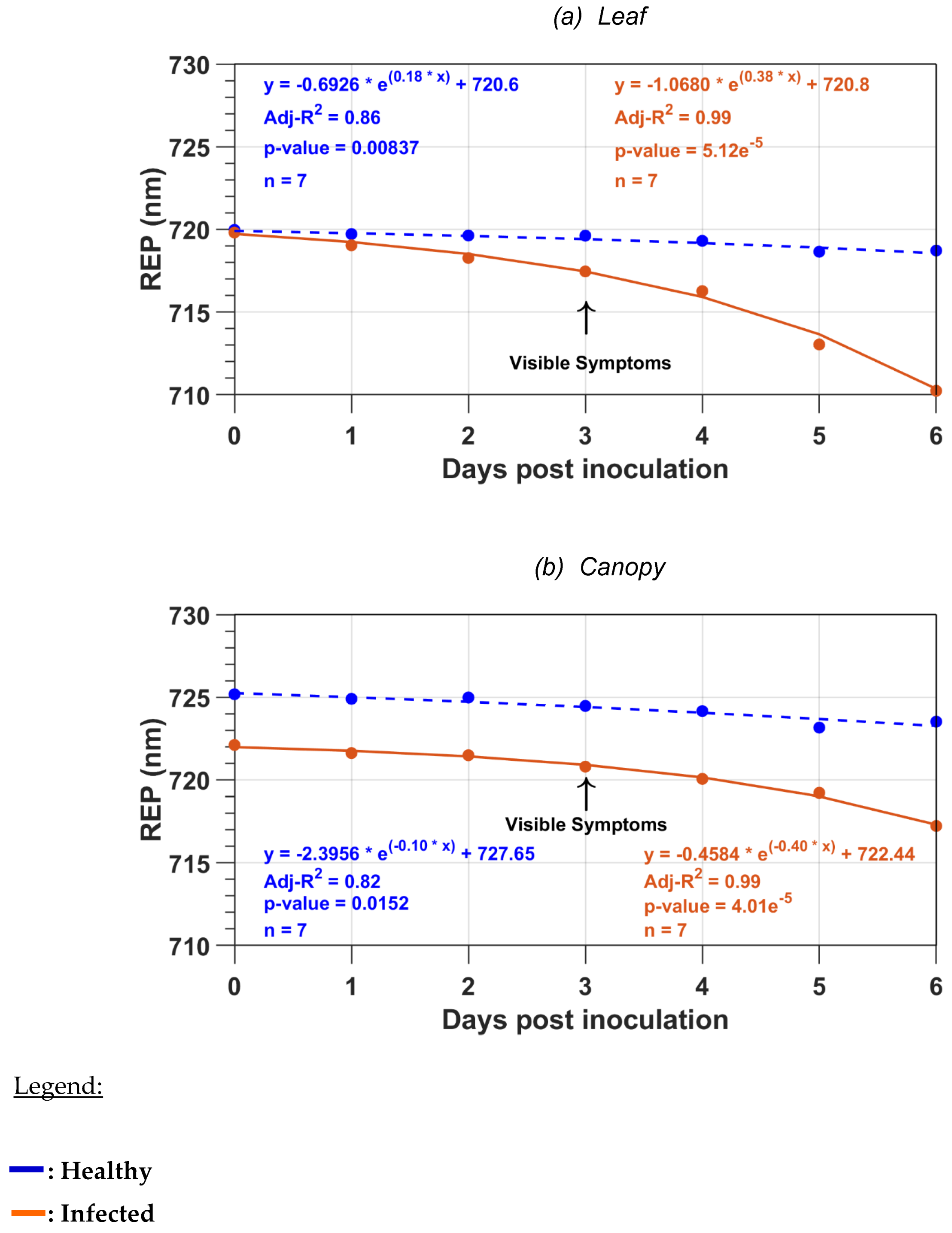
Regression models were used to model the RWP or REP wavelength variations as a function of the DPI. The applied regression methods assume that the data have a normal distribution, which was visually assessed using histogram plots such as for the t-test mean comparison. For both relationships, we tested both the linear and exponential models. The best-explained variance and the lowest sum of the square errors were obtained with a linear model in the case of RWP and an exponential model in the case of REP. The regression model was estimated on a rather small number of observations (n = 7), but each observation was a mean value of more than 100 leaf measurements or 32 canopy measurements for each DPI. Also, the regression parameters were significant, which is an indication that there was no type II error in the models due to the low sample size.

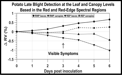
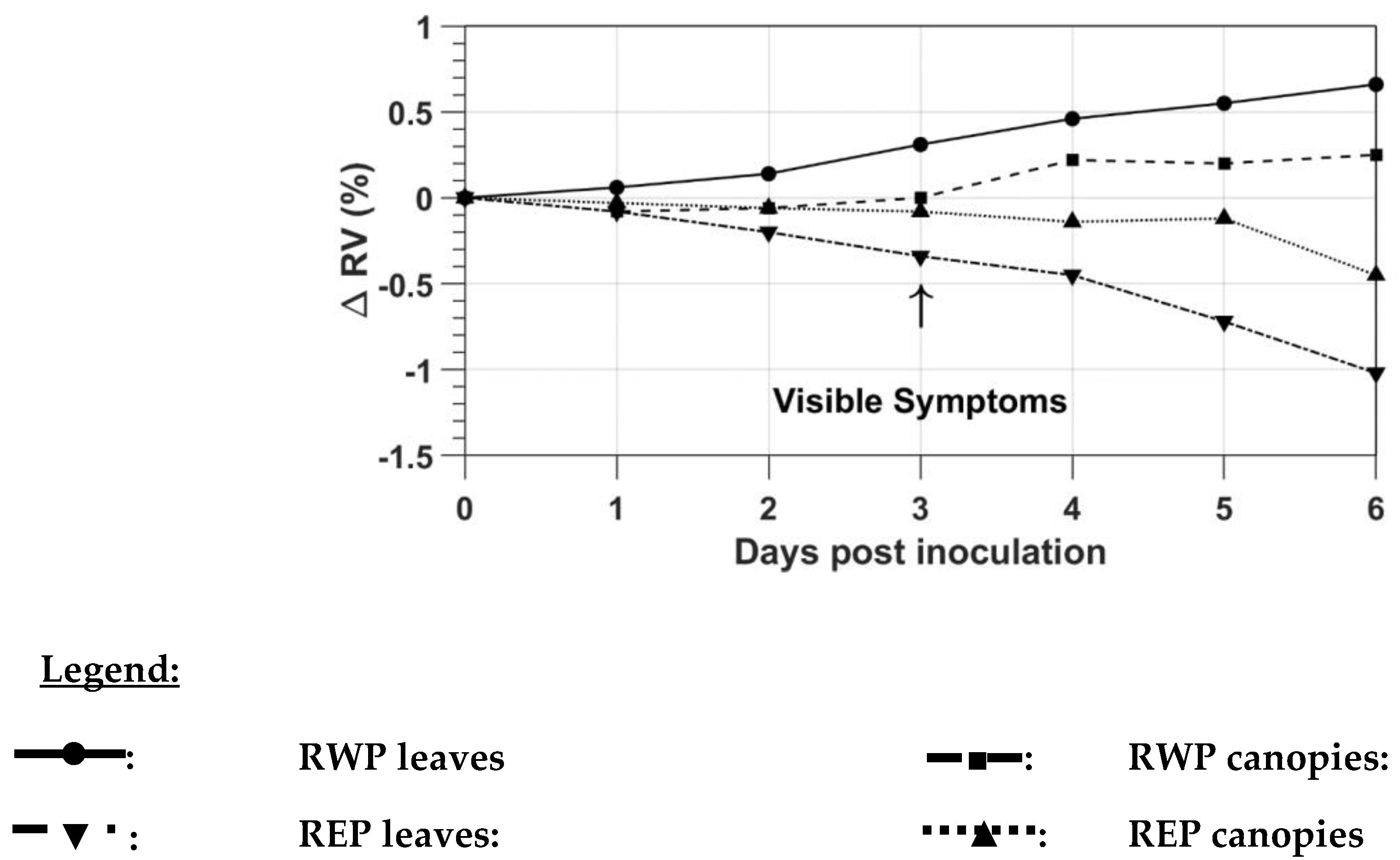
The variations of RWP and REP were also described by the ratio variations (ΔRV), which were computed with the mean daily RWP and REP wavelengths, following Fernández et al. [21], as follows:

ΔRV (%) = 100*[(V_i/V_h) − 1) − (V_i,o/V_h,o) − 1)]

(3)

where

• ΔRV = ratio variation of RWP or REP with respect to the healthy case reported to the day of inoculation (in %);
• V_i = RWP or REP wavelength of the infected leaves or plants (nm);
• V_h = RWP or REP wavelength of the healthy leaves or plants (nm);
• V_i,o = RWP or REP wavelength of the infected leaves or plants on the day of inoculation (nm);
• V_h,o = RWP or REP wavelength of the healthy leaves or plants on the day of inoculation (nm).

Finally, to test whether the RWP, REP, or spectra in the red and red-edge regions sorted healthy and infected leaves or plants, an SVM algorithm embedded in the MATLAB Statistics and Machine Learning Toolbox™ was applied to RWP and REP wavelengths, and the reflectances at 668, 705, 717 and 740 nm were measured at the leaf and canopy levels. These four wavelengths correspond to the central wavelengths of the red and red-edge bands of the Micasense^® Dual-X camera (Micasense, Inc., Seattle, WA, USA) that will be calibrated in field conditions for monitoring the presence of potato late blight from red and red-edge UAV images. The SVM algorithm was calibrated using cross-validation and a 10 K-fold division to avoid overfitting.

3. Results

3.1. Mean Reflectance Spectra

The variations of the reflectance spectra in the red and red-edge regions are presented in Figure 3 and Figure 4 for the leaf and canopy levels, respectively. On the day of inoculation (0 DPI), it is possible to observe that the mean reflectance spectra in the red and red-edge regions of healthy and infected leaves perfectly overlapped (Figure 3a). For the healthy leaves, there were no significant changes as a function of the DPI in the reflectance spectra of the red region (Figure 3a–g). For the infected leaves, there were minor changes in the reflectance spectra in the red region (660–680 nm) from 1 to 4 DPI (Figure 3b–e). At 5 to 6 DPI, the infected leaves had the lowest reflectance in the red region (Figure 3f,g). In the 710–730 nm spectral range of the red-edge region, there were no visible changes in the reflectance spectra of the healthy leaves between the day of inoculation and 6 DPI (Figure 3a–g). By contrast, the reflectance spectra of the infected leaves at 1 DPI had a slight shift towards the shorter wavelengths (Figure 3b). After 1 DPI, there was a constant shift of the wavelengths towards shorter wavelengths (Figure 3c–g). We also observed at 1 DPI higher reflectances for the infected leaves than for the healthy leaves (Figure 3b). However, between 740 to 780 nm, once the symptoms were visible (starting from 3 DPI), the reflectance of the infected leaves was lower than those of the healthy leaves (Figure 3d–g).

Similar to the leaves, no visible changes were detected at the canopy level in the red and red-edge reflectance of the healthy plants from 0 to 6 DPI (Figure 4a–g). For the infected plants, the mean reflectance spectra in the red and red-edge regions perfectly overlapped with those for the healthy plants from the day of inoculation to 3 DPI (Figure 4a–c). At 4 DPI, the first visible changes in the canopy reflectance spectra of the red region (660–680 nm) were observed, with a slight reduction in the reflectance in comparison to the healthy plants. Such minor reduction was also observed at 5 and 6 DPI (Figure 4f,g). Concerning the red-edge region, the canopy spectra between 710 to 730 nm shifted to shorter wavelengths at 3 DPI, when the symptoms were apparent for the first time (Figure 4d). Such a spectral shift to shorter wavelengths is defined as the blue-shift [28]. At 4 DPI, it was possible to observe a separation of both mean spectra of healthy and infected plants between 710 and 730 nm. At 5 and 6 DPI, the separation of both spectra occurred between 700 and 735 nm (Figure 4e–g). The canopy reflectance in the 750–780 nm spectral domain decreased slightly at 5 and 6 DPI (Figure 4f,g).

3.2. First-Order Derivative Spectra

Figure 5 and Figure 6 compared the first-order derivative spectra in the red-edge region as a function of DPI for the healthy and infected leaves and canopies, respectively. At the leaf level, on the day of inoculation, there were no differences between the mean first-order derivative spectra of healthy and infected leaves (Figure 5a). From 1 to 6 DPI, the red-edge FD spectra for the healthy leaves did not vary from one day to another (Figure 5a–g). By contrast, the red-edge FD values of the infected leaves shifted towards shorter wavelengths (blue shift) because of the chlorosis effect due to the disease (Figure 5a–g). At the canopy level, the FD spectra on the day of inoculation perfectly overlapped (Figure 6a). Compared to healthy plants, the FD red-edge of infected plants experienced blue shifts from 2 to 6 DPI (Figure 6), the major blue shift occurring when the symptoms were visible at 6 DPI (Figure 6f). The changes in the red-edge region for the infected plants were stronger than for the healthy plants because of the development of the disease.

3.3. RWP and REP Mean Comparison

The mean and standard deviation of the RWP wavelengths at the leaf and canopy level are presented in

Table 1. Mean and standard variation of the red-well point (RWP) wavelength (in nm) and p-values for the t-test for mean comparison in the case of the leaf and canopy measurements as a function of the number of days post-inoculation (DPI).

DPI	Leaf			Canopy
	Healthy (nm)	Infected (nm)	p-Value	Healthy (nm)	Infected (nm)	p-Value
0	662.65 ± 1.98	662.61 ± 2.04	0.880	665.52 ± 2.20	664.99 ± 2.00	0.325
1	663.02 ± 1.83	663.40 ± 2.49	0.197	666.04 ± 2.39	664.99 ± 2.04	0.067
2	663.17 ± 1.83	664.04 ± 2.30	0.002	666.55 ± 2.32	665.62 ± 2.33	0.119
3	662.86 ± 1.90	664.87 ± 2.89	2.36 × 10−9	666.01 ± 2.35	665.51 ± 2.35	0.402
4	663.86 ± 1.86	666.88 ± 2.99	2.17 × 10−17	665.77 ± 2.51	666.88 ± 2.54	0.160
5	664.65 ± 2.11	668.29 ± 3.57	4.39 × 10−18	667.30 ± 2.29	668.08 ± 2.20	0.179
6	664.32 ± 1.86	668.65 ± 3.39	2.91 × 10−26	667.20 ± 2.32	668.32 ± 1.85	0.039

as a function of the day of inoculation. Table 1 also presents the p-value of a t-test comparing the mean RWP between healthy and infected leaves or canopies as a function of DPI. At the leaf level, the mean RWP was significantly different at p ≤ 0.05 from 2 DPI and at p ≤ 0.001 from 3 to 6 DPI. At the canopy level, the mean RWP was significantly different at p ≤ 0.05 only at 6 DPI.

For REP, the mean and standard deviation of the REP wavelengths at the leaf and canopy level are presented in

Table 2. Mean and standard variation of the red-edge point (REP) wavelength (in nm) and p-values for the t-test for mean comparison in the case of the leaf and canopy measurements as a function of the number of days post-inoculation (DPI).

DPI	Leaf			Canopy
	Healthy (nm)	Infected (nm)	p-Value	Healthy (nm)	Infected (nm)	p-Value
0	718.72 ± 2.05	719.64 ± 1.76	0.753	725.18 ± 1.15	722.11 ± 0.93	4.25 × 10−17
1	719.41 ± 2.24	718.76 ± 2.20	0.028	724.90 ± 1.01	721.62 ± 1.11	4.09 × 10−18
2	719.26 ± 2.43	717.75 ± 3.28	1.20 × 10−4	724.98 ± 0.93	721.49 ± 1.12	6.65 × 10−20
3	719.26 ± 2.44	716.73 ± 3.77	6.32 × 10−9	724.47 ± 1.09	720.80 ± 1.53	4.76 × 10−16
4	718.84 ± 2.87	715.52 ± 4.03	1.17 × 10−11	724.16 ± 1.21	720.06 ± 1.78	1.46 × 10−15
5	717.99 ± 3.39	712.71 ± 5.16	3.32 × 10−17	723.16 ± 1.45	719.22 ± 2.72	1.36 × 10−9
6	718.09 ± 3.41	710.69 ± 6.07	2.74 × 10−24	723.52 ± 1.41	717.23 ± 4.04	1.96 × 10−11

as a function of the day of inoculation. Table 2 also presents the p-value of a t-test comparing the mean REP between healthy and infected leaves or canopies. At the leaf level, the REP position was significantly different at p ≤ 0.05 at 1 DPI and p ≤ 0.001 between 2 and 6 DPI. At the canopy level, a significant difference at p ≤ 0.001was observed since the day of inoculation.

3.4. Modeling of RWP and REP Variations as a Function of DPI

The best fit for the variation of the mean RWP position as a function of the number of days post-inoculation was obtained using a linear regression model with both the leaf and canopy levels (Figure 7). The adjusted R² of the model was significant at p ≤ 0.05 for the healthy leaves (R² = 0.62) and p ≤ 0.001 for the infected leaves (R² = 0.91). At the canopy level, the adjusted R² of the models was lower than for the leaf measurements. It was significant at p ≤ 0.05 for the healthy plants (R² = 0.58) and p ≤ 0.001 for the infected plants (R² = 0.83).

For the REP wavelength, the best fit was obtained with an exponential model for both the leaf- and canopy-level measurements (Figure 8). The models at both the leaf and canopy levels had higher adjusted R² than those for the RWP wavelength, indicating that REP was more sensitive to the disease development than RWP. The adjusted R² of the model was significant at p ≤ 0.01 for the healthy leaves (R² = 0.86) and p ≤ 0.001 for the infected leaves (R² = 0.99). At the canopy level, the adjusted R² of the models was lower than for the leaf measurements, but only for the healthy case. It was significant at p ≤ 0.05 for the healthy plants (R² = 0.82) and p ≤ 0.001 for the infected plants (R² = 0.99).

3.5. RWP and REP Ratio Variation

The ratio variation (ΔRV) for RWP and REP changed starting 1 DPI (Figure 9). At the leaf level, the RWP ratio variations between infected and healthy cases increased from the day of inoculation to 6 DPI, but the REP ratio variations decreased. The change in the ΔRV was stronger for the REP than for the RWP, indicating that REP was more sensitive to the disease development than RWP. The RWP and REP ratio variations between infected and healthy plants were lower than with the leaf measurements. Such as for the leaf measurements, the RWP ratio variations increased from the day of inoculation to 6 DPI, but the REP ratios did not change until 5 DPI and then decreased.

3.6. SVM Classification

SVM classifiers were developed to assess the performance of RWP and REP to discriminate between healthy and infected leaves or plants as a function of DPI. For RWP and REP, the best overall classification accuracy was obtained by applying a linear SVM to the leaf or canopy measurements. For RWP, the related confusion matrix and classification statistics are presented as a function of DPI in

Table 3. Confusion matrix and related statistics when a linear Support Vector Machine (SVM) classifier is applied to the red-well point (RWP) wavelength to classify 124 healthy and 101 infected leaves as a function of the number of days post-inoculation (DPI).

DPI	Class	N	Confusion Matrix			Sensitivity	Specificity	Overall Accuracy (%)
0	H	124		H	I	1	0	55.11
	I	101	H	124	0	0	1
			I	101	0
1	H	124		H	I	1	0	55.11
	I	101	H	124	0	0	1
			I	101	0
2	H	124		H	I	0.9	0.2	58.22
	I	101	H	111	13	0.2	0.9
			I	81	20
3	H	124		H	I	0.83	0.45	65.78
	I	101	H	103	21	0.45	0.83
			I	56	45
4	H	124		H	I	0.84	0.64	75.11
	I	101	H	104	20	0.64	0.84
			I	36	65
5	H	124		H	I	0.89	0.63	77.33
	I	101	H	110	14	0.63	0.89
			I	37	64
6	H	124		H	I	0.88	0.63	76.89
	I	101	H	109	15	0.63	0.88
			I	37	64

and

Table 4. Confusion matrix and related statistics when a linear Support Vector Machine (SVM) classifier is applied to the red-well point (RWP) wavelength to classify 32 healthy and 32 infected spectral observations acquired at canopy level as a function of the number of days post-inoculation (DPI).

DPI	Class	N	Confusion Matrix			Sensitivity	Specificity	Overall Accuracy (%)
0	H	32		H	I	0.56	0.59	57.81
	I	32	H	18	14	0.59	0.56
			I	13	19
1	H	32		H	I	0.53	0.63	57.81
	I	32	H	17	15	0.63	0.53
			I	12	20
2	H	32		H	I	0.66	0.47	56.25
	I	32	H	21	11	0.47	0.66
			I	17	15
3	H	32		H	I	0.59	0.56	57.81
	I	32	H	19	13	0.56	0.59
			I	14	18
4	H	32		H	I	0.59	0.56	57.81
	I	32	H	19	13	0.56	0.59
			I	14	18
5	H	32		H	I	0.38	0.63	50
	I	32	H	12	20	0.63	0.38
			I	12	20
6	H	32		H	I	0.47	0.72	59.38
	I	32	H	15	17	0.72	0.47
			I	9	23

for the leaf and canopies measurements, respectively. At the leaf level, the overall classification accuracy increased from 0 DPI to reach a maximum of 77.33% at 5 DPI and then decreased slightly. The highest increase occurred at 3 DPI when the symptoms were visible (Table 3). On the day of inoculation (0 DPI), the sensitivity and specificity had both a value of 1.0 (Table 3). This means that the linear SVM was able to properly classify all the leaves in the healthy group with RWP. Indeed, at 0 DPI, both the healthy and infected leaves had similar RWP values as the disease was not yet developed (Table 1). At 3 DPI, when the symptoms were visible for the first time, the sensitivity of the infected leaves increased to 0.45, meaning that 45% of infected leaves were properly classified by the linear SVM applied to RWP. From 3 to 6 DPI the sensitivity of the infected leaves increased up to 63% because of the increased impact of the disease development on the RWP values.

At the canopy level (Table 4), the overall classification accuracy was lower than at the leaf level. It was almost constant (57%) until 5 DPI, then dropped, and then increased again to reach its maximum of 59.38% at 6 DPI. The lower classification accuracy obtained with the RWP values at the canopy level can be explained by the lack of difference in the RWP values between the healthy and infected canopies (Table 1). On the day of inoculation (0 DPI), the sensitivity and specificity of the healthy (infected) canopies had values of 0.56 (0.59) and 0.59 (0.56), respectively. Theoretically, the sensitivity for the healthy plants should be equal to 1 because all the plants should be classified in the healthy group since the disease is not yet developed. While the RWP values were not significantly different between healthy and infected plants (Table 1), the fact that the sensitivity was lower than 1.0 for the healthy plants means that some of the plants were classified in the infected group instead of being classified in the healthy group, as they were different than the plants of the healthy group.Both factors were not considered in the analysis as we did not measure the leaf area indices nor the leaf angle distributions. From 2 to 3 DPI, when the symptoms were visible for the first time, the sensitivity of the infected plants increased from 0.47 to 0.56, meaning that 56% of infected canopy spectra were properly classified by the linear SVM. From 4 to 6 DPI the sensitivity of the infected canopies increased from 0.56 to 0.72 because of the impact of the disease development on the RWP values.

The results corresponding to REP are presented in

Table 5. Confusion matrix and related statistics when a linear Support Vector Machine (SVM) classifier is applied to the red-edge point (REP) wavelength to classify 124 healthy and 101 infected leaves as a function of the number of days post-inoculation (DPI).

DPI	Class	N	Confusion Matrix			Sensitivity	Specificity	Overall Accuracy (%)
0	H	124		H	I	1	0	55.11
	I	101	H	124	0	0	1
			I	101	0
1	H	124		H	I	0.95	0.02	53.33
	I	101	H	118	6	0.02	0.95
			I	99	2
2	H	124		H	I	0.9	0.2	58.67
	I	101	H	112	12	0.2	0.9
			I	81	20
3	H	124		H	I	0.85	0.29	59.56
	I	101	H	105	19	0.29	0.85
			I	72	29
4	H	124		H	I	0.86	0.47	68.44
	I	101	H	107	17	0.47	0.86
			I	54	47
5	H	124		H	I	0.88	0.55	73.33
	I	101	H	109	15	0.55	0.88
			I	45	56
6	H	124		H	I	0.9	0.57	75.56
	I	101	H	112	12	0.57	0.9
			I	45	58

for the leaf measurements and in

Table 6. Confusion matrix and related statistics when a linear Support Vector Machine (SVM) classifier is applied to the red-edge point (REP) wavelength to classify 32 healthy and 32 infected spectral observations acquired at canopy level as a function of the number of days post-inoculation (DPI).

DPI	Class	N	Confusion Matrix			Sensitivity	Specificity	Overall Accuracy (%)
0	H	32		H	I	0.94	0.94	93.75
	I	32	H	30	2	0.94	0.94
			I	2	30
1	H	32		H	I	0.97	0.88	92.19
	I	32	H	31	1	0.88	0.97
			I	4	28
2	H	32		H	I	0.94	1	96.88
	I	32	H	30	2	1	0.94
			I	0	32
3	H	32		H	I	0.91	0.94	92.19
	I	32	H	29	2	0.94	0.91
			I	2	30
4	H	32		H	I	0.97	0.97	96.88
	I	32	H	31	1	0.97	0.97
			I	1	31
5	H	32		H	I	0.88	0.84	85.94
	I	32	H	28	4	0.84	0.88
			I	5	27
6	H	32		H	I	0.88	0.91	89.06
	I	32	H	28	4	0.91	0.88
			I	3	29

for the canopy measurements. At the leaf level (Table 5), the overall classification accuracy was on the same order of magnitude as the one for RWP whatever the DPI. It increased from 0 to 6 DPI when it reached a maximum (75.56%). On the day of inoculation (0 DPI), the sensitivity and specificity had a value of 1.0 similar to RWP. This means that the linear SVM was able to properly classify all the healthy leaves. Indeed, at 0 DPI, both the healthy and infected leaves had similar REP values as the disease was not yet developed (Table 2). At 3 DPI, when the symptoms were visible for the first time, the sensitivity of the infected leaves increased to 0.29, meaning that 29% of infected leaves were properly classified by the linear SVM. From 3 to 6 DPI, the sensitivity of the infected leaves increased up to 0.57 because of the increased impact of the disease development on the REP values.

At the canopy level (Table 6), the overall classification accuracy was higher than at the leaf level. It was almost constant (higher than 90%) until 4 DPI, then dropped to 85.94%, and then increased again to 89.06% at 6 DPI. The high classification accuracy obtained with the REP values at the canopy level can be explained by the significant difference (p ≤ 0.001) in the REP values between the healthy and infected canopies (Table 2). The sensitivity fluctuated between 0.94 (0 DPI) to 0.88 (6 DPI) for the healthy canopies. For the infected plants, the sensitivity increased from 0.88 (1 DPI) to 1.00 (2 DPI), but then it decreased to 0.94 at 3 DPI, increased to 0.97 at 4 DPI, decreased to 0.84 at 5 DPI, and finally increased to 0.91 at 6 DPI. Theoretically, the sensitivity for the healthy plants at 0 DPI should be equal to 1.0 because all the plants should be classified in the healthy group since the disease is not yet developed. A sensitivity lower than 1.0 for the healthy plants means that plants were classified in the infected group instead of the healthy group given that both groups have a significantly different mean REP value. As shown in Table 2, on the day of inoculation (0 DPI), the REPs of healthy and infected canopies had a significant (at p < 0.05) difference of about 3 nm.

Because the purpose of this study was to test UAV images to detect late blight disease over potato fields, an SVM classifier was also applied to reflectances at the central wavelengths of the four red and red-edge bands of the Micasense^® Dual-X camera, i.e., 668, 705, 717 and 740 nm. The best overall classification accuracy was achieved by applying a quadratic SVM classifier for the leaf measurements (

Table 7. Confusion matrix and related classification statistics when a Quadratic Support Vector Machine (SVM) classifier is applied to the reflectance at 668 ¹, 705 ², 717 ³ and 740 ⁴ nm to classify 124 healthy and 101 infected leaves as a function of the days post-inoculation (DPI).

DPI	Class	N	Confusion Matrix			Sensitivity	Specificity	Overall Accuracy (%)
0	H	124		H	I	0.79	0.46	64
	I	101	H	98	26	0.46	0.79
			I	55	46
1	H	124		H	I	0.81	0.54	69.3
	I	101	H	101	23	0.54	0.81
			I	46	55
2	H	124		H	I	0.77	0.56	67.56
	I	101	H	95	29	0.56	0.77
			I	44	57
3	H	124		H	I	0.94	0.84	89.33
	I	101	H	116	8	0.84	0.94
			I	16	85
4	H	124		H	I	0.92	0.89	90.67
	I	101	H	114	10	0.89	0.92
			I	11	90
5	H	124		H	I	0.98	0.77	88.89
	I	101	H	122	2	0.77	0.98
			I	23	78
6	H	124		H	I	0.96	0.9	93.33
	I	101	H	119	5	0.9	0.96
			I	10	91

¹ Central wavelength of the red band (663–673 nm) of the MicaSense RedEdge-MX Dual Camera; ² central wavelength of the first red edge-band ((700–710 nm) of the MicaSense RedEdge-MX Dual Camera; ³ central wavelength of the second red-edge band (712–722 nm) of the MicaSense RedEdge-MX Dual Camera; ⁴ central wavelength of the third red-edge band (731–749 nm) of the MicaSense RedEdge-MX Dual Camera.

) and a cubic SVM for the canopy measurements (

Table 8. Confusion matrix and related classification statistics when a Cubic Support Vector Machine classifier is applied to the reflectance at 668 ¹, 705 ², 717 ³ and 740 ⁴ nm to classify 32 healthy and 32 infected spectral observations acquired at canopy level as a function of the number of days post-inoculation (DPI).

DPI	Class	N	Confusion Matrix			Sensitivity	Specificity	Overall Accuracy (%)
0	H	32		H	I	0.69	0.56	62.5
	I	32	H	22	10	0.56	0.69
			I	14	18
1	H	32		H	I	0.59	0.72	65.63
	I	32	H	19	13	0.72	0.59
			I	9	23
2	H	32		H	I	0.59	0.72	65.63
	I	32	H	19	13	0.72	0.59
			I	9	23
3	H	32		H	I	0.66	0.47	56.25
	I	32	H	21	11	0.47	0.66
			I	17	15
4	H	32		H	I	0.74	0.76	75
	I	32	H	23	8	0.76	0.74
			I	8	25
5	H	32		H	I	0.97	0.82	89.06
	I	32	H	30	1	0.82	0.97
			I	6	27
6	H	32		H	I	0.78	0.91	84.38
	I	32	H	25	7	0.91	0.78
			I	3	29

¹ Central wavelength of the red band (663–673 nm) of the MicaSense RedEdge-MX Dual Camera; ² central wavelength of the first red edge-band (700–710 nm) of the MicaSense RedEdge-MX Dual Camera; ³ central wavelength of the second red-edge band (712–722 nm) of the MicaSense RedEdge-MX Dual Camera; ⁴ central wavelength of the third red-edge band (731–749 nm) of the MicaSense RedEdge-MX Dual Camera.

). Overall, the SVM classification of healthy and infected leaves or plants was better with the reflectance at 668, 705, 717 and 740 nm than with RWP or REP. At the leaf level (Table 7), the overall classification accuracy increased from 64.00% at 0 DPI to reach 93.33% at 6 DPI with the disease development. The corresponding sensitivities of the infected leaves increased from 0.46 at 0 DPI to 0.84 at 3 DPI when the first symptoms were visible, meaning that the quadratic SVM can sort healthy and infected leaves from the beginning of the necrotic stage of the disease development. The highest sensitivity (0.90) for the infected case was reached at 6 DPI when the leaves presented more advanced symptoms of the disease. Throughout the evaluation period, the sensitivity for the healthy leaves was never below 0.77, meaning that the quadratic SVM can sort healthy and infected leaves using only four reflectances related to the red and red-edge regions. At the canopy level (Table 8), the overall classification accuracy was lower than at the leaf level. The sensitivity of the infected plants increased from 0 DPI (0.56) to 6 DPI (0.91). The low sensitivity for the infected canopies and low overall accuracy at 3 DPI might be due to measurement errors.

4. Discussion

In this study, we analyzed the changes in the raw and first-order derivative reflectance spectra in the red and red-edge regions induced by late blight disease on potato leaves and plants. In our experiment, the pre-symptomatology period has the same length as the one of Gold et al. [22] but a shorter length than those observed by Schumann [30]. Our study and Gold et al. [22] used data acquired in a growth chamber that provides optimal conditions for disease development. By contrast, Schumann [30] reported field results, where the development of the disease depends on weather conditions and can take more time to be developed. For both the raw and first-order derivative spectra, the disease induces chlorosis that produces a blue shift. At the plant level, the first-order derivative reflectance spectra were more sensitive to the disease development than the raw reflectance spectra, given that the blue shift was observed at 2 DPI before the symptoms were visible with the first-order derivative reflectance spectra but only at 4 DPI after the symptoms were visible with the raw reflectance spectra. The reason for the high sensitivity of first-order derivative spectra is probably because first-order derivatives suppress the spectral effect of other organic components present in leaves, like lignin and secondary pigments [28], therefore improving the sensitivity to chlorosis. We also observed an increase in the raw reflectance values in the red-edge region that was determined by Carter and Knapp [31] as being an early indicator of stress.

The raw and first-order derivative reflectance spectra were used to derive two main parameters of the red and red-edge region: the RWP and REP wavelengths. The REP wavelength was shown to be more sensitive to the disease than the RWP. As a result, the modeling of the variation as a function of DPI produced models with higher R² values with the REP values than with the RWP values. The blue shift we observed with REP is in agreement with several studies [32,33,34] that related this blue shift to chlorosis and plant stress. Our result with the RWP is not in agreement with Liu et al. [35], who reported a high sensitivity of RWP to chlorophyll content. Results of Liu et al. [35] were based on simulations, while our results are based on measurements. Another difference with this study is that Liu et al. [35] used an inverted Gaussian model to estimate RWP while we searched for the minimum reflectance value of a quadratic curve.

Following Dutta et al. [18] and Fernández et al. [21], we also computed the percentual variations of the ratio between the infected and healthy cases (ΔRV). Our ratio variations computed with the RWP and REP values at the leaf and canopy levels (−1.02% to 0.66%) are lower than the NDVI-based ratio variations computed by Dutta et al. [18] (−24% to −60%) with AWiFS and MODIS data over four potato sites infected with late blight, probably because for Dutta et al. [18] the variation was computed over a longer period (24 days between the first and last evaluations) compared to our period (6 days between the first and last evaluations). The variations observed for both the RWP and REP wavelengths were also lower than those computed by Fernández et al. [21] with the simple ratio [36] and the red-edge chlorophyll index [37] on the same dataset as the one used in this study. In this study, the variations are computed based on single wavelength positions (RWP and REP), while those of Fernández et al. [21] use vegetation index values that are computed using reflectance in multiple bands.

We applied an SVM classifier to RWP or REP wavelengths as well as to reflectance values at the four red and red-edge wavelengths of the Micasense camera to sort healthy and infected leaves or plants. SVM classifiers were already determined to be highly performant even in the case of limited samples [38]. The classifiers applied to RWP or REP were less performant than the ones applied to the reflectances of the four Micasense bands. At the canopy level, both the overall classification accuracy (93%) and the sensitivity (0.94) were high with both the healthy and infected plants at 0 DPI when using REP (Table 6). As shown in Table 2, there was a significant (at p < 0.05) difference of the REP values between the healthy and infected groups. Such difference may be due to a difference in leaf area index or leaf angle distribution between both groups of plants. This difference was not quantified in the analysis as we did not measure the leaf area indices nor the leaf angle distributions. Differences in leaf area indices or leaf angle distributions have already been shown to influence REP [32,39]. Using the reflectances at the four red and red-edge wavelengths of the Micasense camera, at the leaf level (Table 7), the overall classification accuracy and the sensitivities for the infected leaves increased when the first symptoms were visible at 3 DPI. The quadratic SVM could sort healthy and infected leaves, particularly when the symptoms became apparent. The highest classification accuracy (93.33%) and the highest sensitivity (0.90) for the infected case were obtained at 6 DPI once the disease was well established. This accuracy was on the same order of magnitude as the one (93.0%) obtained at 4 DPI by Römer et al. [40] who applied an SVM classifier to ultraviolet-induced fluorescence data acquired between 370 to 800 nm for classifying healthy leaves and leaves infected with Puccinia triticia in the case of winter wheat (Triticum aestivum). It was higher than the one obtained with a Partial Least Square Discriminant Analysis (PLS-DA) method for sorting leaves infected with potato late blight (89.77% [21] and 65–72.73% [41]). At the canopy level, the highest classification accuracy was obtained at 5 DPI (89.06%,). It was higher than the one (85.93%) obtained by Fernández et al. [21] who applied PLS-DA to the 400–900 reflectance spectra to classify healthy and infected plants.

Finally, a factor that needs to be considered as having a potential influence on the classification results at the canopy level is related to the measured area on each plant. As explained in the Materials and Methods, the measured area on each healthy or infected plant was 82.83 cm², and the total plant area was 490.87 cm². Hence, only 16.87% of the entire canopy area was measured. This measured area is lower than the one of Zhang et al. [16], who acquired spectra on a measured area of 5658 cm² on tomato plants infected with late blight and of Bienkowski et al. [42] who collected spectral data on a measured area of 1520 cm². However, both studies did not report the percentage of the plant area; the measurements were done in field conditions. Our spectral data were collected on plants grown in pots inside a walk-in chamber. Therefore, the influence of factors such as illumination and canopy plant geometry might be lower in our case than in the case of the aforementioned studies.

5. Conclusions

In this study, we analyzed the changes in the raw and first-order derivative reflectance spectra in the red and red-edge regions induced by late blight disease on potato leaves and plants. At the leaf level, with the disease development, both types of spectra had a blue spectral shift due to the chlorosis induced by the disease. The blue shift appeared earlier in the first-order derivative reflectance spectra than in the raw reflectance spectra. We also observed an increase in the raw leaf reflectance values in the red-edge region that can be an early indicator of stress. At the canopy level, the spectra were less sensitive to disease development than the leaf spectra. Such as for the leaf level, the first-order derivative spectra were also better than the raw reflectance spectra to detect the disease. Both types of spectra were used to compute two main parameters of the red and red-edge region: the RWP and REP wavelengths. The REP wavelength was shown to be more sensitive to the disease than the RWP for both the leaf and canopy measurements. The models of the variations as a function of DPI had higher R² values with REP than with RWP. Following Dutta et al. [18] and Fernández et al. [21], we also computed the percent variations of the ratio between the infected and healthy cases (ΔRV). The variations observed for both the RWP and REP wavelengths were lower than those of [18] and [21]. To sort healthy and infected leaves or plants, we applied an SVM classifier to RWP or REP wavelengths as well as to reflectance at four selected red and red-edge bands of the Micasense^® Dual-X camera. The SVM classifier applied to these reflectances gave higher overall accuracies that the SVM classifier applied to the REP and RWP values. The SVM classifier applied to reflectances of four Micasense^® Dual-X camera bands in the red and red-edge regions was able to sort healthy and infected cases with both leaf and canopy measurements, reaching an overall classification accuracy of 89.33% at 3 DPI when symptoms were visible for the first time with the leaf measurements and of 89.06% at 5 DPI, i.e., two days after the symptoms became apparent, with the canopy measurements.

Our results were obtained on Shepody cultivar potato plants. Further work is needed to test the method over other potato cultivars. This is especially important for the canopy-level results because the canopy-level measurements are influenced by the canopy geometry, which highly depends on the cultivar. Future research under controlled environments should investigate whether the size of the canopy areas considered for the spectral acquisition has an influence on the capacity of red and red-edge regions to detect late blight over potato plants. Additionally, the results were obtained in a walk-in chamber that had a controlled environment. Further work is needed to test the methodology in real field conditions. The study used point measurements, and there is the need to test the methodology on UAV imagery acquired over real field conditions. For field condition testing, it is important to determine the optimal spatial and temporal resolutions of the UAV images to be able to effectively monitor the disease occurrence in the field, as it is critical to get the information about the disease on its onset to have proper disease management strategies. While the results of this study are quite promising, they were acquired on a limited number of plants. Further work is needed to test the method of broad sampling. In this study, we only tested two metrics, REP and RWP, but other spectral metrics that can detect crop diseases can be considered, such as those already tested by past studies working on various crop diseases (

Table 9. Literature comparison of spectral variables tested for detect crop diseases.

Disease	Vegetation Index (*)	Authors
Potato late blight	SR, Clgreen, RI, TCARI, TCARI/OSAVI-2, ClRed-Edge, Red-Edge NDVI.	Fernández et al. [21]
Potato late blight	NDSI between 400 and 2400 nm.	Gold et al. [22,41]
Pear fire blight	SIPI, RDVI, MSR, NRI, MCARI1, MCARI2, TVI, MTVI1, MTVI2, TCARI, PSRI, ARI	Bagheri [43]
Wheat yellow rust	NRI, GI, GLI, ARI, GNDVI, TVI, CIG, TGI, NDVI, SAVI, SR, OSAVI, CIRE, EVI, TCARI, CVI, SCCCI	Su et al. [44]

(*) SR = Simple Ratio [36]; Clgreen = Green Chlorophyll index [37]; ClRed-Edge = Red-Edge Chlorophyll index [37]; RI = Redness Index [45]; TCARI = Transformed Chlorophyll Absorption [46]; TCARI/OSAVI-2 = Transformed Chlorophyll Absorption/Optimized Soil-Adjusted Vegetation Index 2 ratio [47]; Red-Edge NDVI = Red-Edge Normalized Difference Vegetation Index [48]; NDSI = Normalized Spectral Differences Indices [22,41]; SIPI = Structure Intensive Pigment Index [49]; RDVI = Randomized Difference Vegetation Index [50]; MSR = Modified Simple Ratio [50]; NRI = Nitrogen Reflectance Index [46]; MCARI1 = Modified Triangular Vegetation Index [51]; MCARI2 = Modified Triangular Vegetation Index 2 [51]; TVI = Triangular Vegetation Index [52]; PSRI = Plant Senescence Reflectance Index [46]; ARI = Anthocyanin Reflectance Index [53]; GI = Greenness Index [54]; GLI = Green Leaf Index [55]; GNDVI = Green Normalized Difference Vegetation Index [56]; CIG = Chlorophyll Index-Green [57]; TGI = Triangular Greenness Index [58]; NDVI = Normalized Difference Vegetation Index [59]; SAVI = Soil Adjusted Vegetation Index [60]; OSAVI = Optimized Soil Adjusted Vegetation Index [61]; CIRE = Chlorophyll Index-RedEdge [57]; EVI = Enhanced Vegetation Index [62]; CVI = Chlorophyll Vegetation Index [63]; SCCCI = Simplified Canopy Chlorophyll Content Index [64].

).

References

1. Hardwick, N.V. Disease forecasting. In The Epidemiology of Plant Diseases, 2nd ed.; Cooke, B.M., Jones, D.G., Kaye, B., Eds.; Springer: Dordrecht, The Netherlands, 2006; pp. 239–267. [Google Scholar]
2. Van Aubel, G.; Serderidis, S.; Ivens, J.; Clinckemaillie, A.; Legrève, A.; Hause, B.; Van Cutsem, P. Oligosaccharides successfully thwart hijacking of the salicylic acid pathway by Phytophthora infestans in potato leaves. Plant Pathol. 2018, 67, 1901–1911. [Google Scholar] [CrossRef] [Green Version]
3. Hansen, Z.R.; Knaus, B.J.; Tabima, J.F.; Press, C.M.; Judelson, H.S.; Grunwald, N.J.; Smart, C.D. Loop-mediated isothermal amplification for detection of the tomato and potato late blight pathogen, Phytophthora infestans. J. Appl. Micobiol. 2016, 120, 1010–1020. [Google Scholar] [CrossRef] [PubMed] [Green Version]
4. Ray, M.; Ray, A.; Dash, S.; Mishra, A.; Achary, K.G.; Nayak, S.; Singh, S. Fungal disease detection in plants: Traditional assays, novel diagnostic techniques, and biosensors. Biosens. Bioelectron. 2017, 87, 708–723. [Google Scholar] [CrossRef]
5. Zhang, M.; Qin, Z.; Liu, X. Remote sensed spectral imagery to detect late blight in field tomatoes. Precis. Agric. 2005, 6, 489–508. [Google Scholar] [CrossRef]
6. Knipling, E.B. Physical and physiological basis for the reflectance of visible and near-infrared radiation from vegetation. Remote Sens. Environ. 1970, 1, 155–159. [Google Scholar] [CrossRef]
7. Taoutaou, A.; Socaciu, C.; Pamfil, D.; Fetea, F.; Balazs, E.; Botez, C. Fourier-transformed infrared spectroscopy applied for studying compatible interaction in the pathosystem Phytophthora infestans-Solanum tuberosum. Not. Bot. Hortic. Agrobot. Cluj Napoca 2012, 38, 69–75. [Google Scholar] [CrossRef]
8. Mutanga, O.; Skidmore, A.K. Red edge shift and biochemical content in grass canopies. ISPRS J. Photogramm. Remote Sens. 2007, 62, 34–42. [Google Scholar] [CrossRef]
9. Horler, D.N.H.; Dockray, M.; Barber, J. The red edge of plant leaf reflectance. Int. J. Remote Sens. 1983, 4, 273–288. [Google Scholar] [CrossRef]
10. Delegido, J.; Verrelst, J.; Meza, C.M.; Rivera, J.P.; Alonso, L.; Moreno, J. A red-edge spectral index for remote sensing estimation of green LAI over agroecosystems. Eur. J. Agron. 2013, 46, 42–52. [Google Scholar] [CrossRef]
11. Pu, R.; Gong, P.; Biging, G.S.; Larrieu, M.R. Extraction of red edge optical parameters from Hyperion data for estimation of forest leaf area index. IEEE Trans. Geosci. Remote Sens. 2003, 41, 916–921. [Google Scholar] [CrossRef] [Green Version]
12. Darvishzadeh, R.; Atzberger, C.; Skidmore, A.K.; Abkar, A.A. Leaf area index deviation from hyperspectral vegetation indices and the red edge position. Int. J. Remote Sens. 2009, 30, 6199–6218. [Google Scholar] [CrossRef]
13. Hardham, A.R. Cell biology of plant-oomycete interactions. Cell. Microbiol. 2007, 9, 31–39. [Google Scholar] [CrossRef] [PubMed]
14. Zuluaga, A.P.; Vega-Arreguin, J.C.; Fei, Z.; Ponnala, L.; Lee, S.L.; Matas, A.J.; Patev, S.; Fry, W.E.; Rose, J.K.C. Transcriptional dunamcs of Phytophthora infestans during sequential stages of hemibiotrophic infection of tomato. Mol. Plant Pathol. 2016, 17, 29–41. [Google Scholar] [CrossRef] [PubMed]
15. Peng, Y.; Gitelson, A.A.; Keydan, G.; Rundquist, D.C.; Moses, W. Remote estimation of gross primary production in maize and support for a new paradigm based on total crop chlorophyll content. Remote Sens. Environ. 2011, 115, 978–989. [Google Scholar] [CrossRef]
16. Zhang, M.; Liu, X.; O’Neill, M. Spectral discrimination of Phytophthora infestans infection on tomatoes based on principal component and cluster analyses. Int. J. Remote Sens. 2002, 23, 1095–1107. [Google Scholar] [CrossRef]
17. Zhang, M.; Qin, Z.; Liu, X.; Ustin, S.L. Detection of stress in tomatoes induced by late blight disease in California, USA, using hyperspectral remote sensing. Int. J. Appl. Earth Obs. 2003, 4, 295–310. [Google Scholar] [CrossRef]
18. Dutta, S.; Singh, S.K.; Panigrahy, S. Assessment of late blight induced diseased potato crops: A case study for West Bengal district using temporal AWiFS and MODIS data. J. Indian Soc. Remote Sens. 2014, 42, 353–361. [Google Scholar] [CrossRef]
19. Ray, S.S.; Jain, N.; Arora, R.K.; Chavan, S.; Panigrahy, S. Utility of hyperspectral data for potato late blight disease detection. J. Indian Soc. Remote Sens. 2011, 39, 161–169. [Google Scholar] [CrossRef]
20. Franceschini, M.H.D.; Bartholomeus, H.; Van Apeldoorn, D.; Suomalainen, J.; Kooistra, L. Assessing changes in potato canopy caused by late blight in organic production systems through UAV-based pushbroom imaging spectrometer. In Proceedings of the International Archives Photogrammetry, Remote Sensing, and Spatial Information Science, Conference on Unmanned Aerial Vehicles in Geomatics, Bonn, Germany, 4–7 September 2017; Volume 42, pp. 109–112. [Google Scholar] [CrossRef] [Green Version]
21. Fernández, C.I.; Leblon, B.; Haddadi, A.; Wang, J.; Wang, K. Potato late blight detection at leaf and canopy levels. Can. J. Remote Sens. 2020, in press. [Google Scholar]
22. Gold, M.K.; Townsend, P.A.; Chlus, A.; Herrmann, I.; Couture, J.J.; Larson, E.R.; Gevens, A.J. Hyperspectral measurements enable pre-symptomatic detection and differentiation of contrasting physiological effects of late blight and early blight in potato. Remote Sens. 2020, 12, 286. [Google Scholar] [CrossRef] [Green Version]
23. Mountrakis, G.; Im, J.; Ogole, C. Support vector machine in remote sensing: A review. J. Photogramm. Remote Sens. 2011, 66, 247–259. [Google Scholar] [CrossRef]
24. Savitzky, A.; Golay, M.J.E. Smoothing and differentiation of data by simplified least-squares procedures. Anal. Chem. 1964, 36, 1627–1639. [Google Scholar] [CrossRef]
25. Isaksson, T.; Næs, T. The effect of multiplicative scatter correction (MSC) and linearity improvement in NIR spectroscopy. Appl. Spectrosc. 1988, 42, 1273–1284. [Google Scholar] [CrossRef]
26. Boochs, F.; Kupfer, G.; Dockter, K.; Kuhbauch, W. Shape of the red edge as vitality indicator for plants. Int. J. Remote Sens. 2007, 11, 1741–1753. [Google Scholar] [CrossRef]
27. ASD Inc. ViewSpec PROTM User Manual; Document 600555 Rev. A©; ASD Inc.: Boulder, CO, USA, 2008; p. 28. [Google Scholar]
28. Dawson, T.P.; Curran, P.J. A new technique for interpolating the reflectance red-edge position. Int. J. Remote Sens. 1998, 19, 2133–2139. [Google Scholar] [CrossRef]
29. Posten, H.O. Robustness of the two-sample t-test. In Robustness of Statistical Methods and Nonparametric Statistics. In Theory and Decision Library (Series B: Mathematical and Statistical Methods); Springer: Dordrecht, The Netherlands, 1984; Volume 1, pp. 92–99. [Google Scholar] [CrossRef]
30. Schumann, G.L. Introduction to the fungi and their life. In Plant Diseases: Their Biology and Social Impact, 1st ed.; The American Phytopathological Society Press: Saint Paul, MN, USA, 1991; pp. 25–46. [Google Scholar]
31. Carter, G.A.; Knapp, A.K. Leaf optical properties in higher plants: Linking spectral characteristics to stress and chlorophyll concentration. Am. J. Bot. 2001, 88, 677–684. [Google Scholar] [CrossRef] [Green Version]
32. Rock, B.N.; Hoshizaki, T.; Miller, J.R. Comparison of in situ and airborne spectral measurements of the blue shift associated with forest decline. Remote Sens. Environ. 1988, 24, 109–127. [Google Scholar] [CrossRef]
33. Gitelson, A.A.; Merzlyak, M.N.; Lichtenthaler, H.K. Detection of red edge position and chlorophyll content by reflectance measurements near 700 nm. J. Plant Physiol. 1996, 148, 501–508. [Google Scholar] [CrossRef]
34. Baranoski, G.V.; Rokne, J.G. A practical approach for estimating the red edge position of plant leaf reflectance. Int. J. Remote Sens. 2005, 26, 503–521. [Google Scholar] [CrossRef]
35. Liu, J.; Miller, R.; Haboudane, D.; Pattey, E. Exploring the relationship between red edge parameters and crop variables for precision agriculture. In Proceedings of the IEEE International Geoscience and Remote Sensing Symposium (IGARSS’04), Anchorage, AK, USA, 20–24 September 2004; pp. 1276–1279. [Google Scholar]
36. Jordan, C.F. Derivation of leaf area index from quality of light on the forest floor. Ecology 1969, 50, 663–666. [Google Scholar] [CrossRef]
37. Gitelson, A.A.; Viña, A.; Ciganda, V.; Rundquist, D.C.; Arkebauer, T.J. Remote estimation of canopy chlorophyll content in crops. Geophy. Res. Lett. 2005, 32, 20–26. [Google Scholar] [CrossRef] [Green Version]
38. Zhang, J.; Huang, Y.; Pu, R.; Gonzalez-Moreno, P.; Yuan, L.; Wu, K.; Huang, W. Monitoring plant diseases and pest through remote sensing technology: A review. Comput. Electron. Agric. 2019, 165, 10493. [Google Scholar] [CrossRef]
39. Boni-Vicari, M.; Pisek, J.; Disney, M. New estimates of leaf angle distribution from terrestrial LiDAR: Comparison with measured and modelled estimates from nine broadleaf tree species. Agric. For. Meteorol. 2019, 264, 322–333. [Google Scholar] [CrossRef]
40. Römer, C.; Bürling, K.; Hunsche, M.; Rumpf, T.; Noga, G.; Plümer, L. Robust fitting of fluorescence spectra for pre-symptomatic what leaf rust detection with Support Vector Machines. Comput. Electron. Agric. 2011, 79, 180–188. [Google Scholar] [CrossRef]
41. Gold, M.K.; Townsend, P.A.; Herrmann, I.; Gevens, A.J. Investigating potato late blight physiological differences across potato cultivars with spectroscopy and machine learning. Plant Sci. 2019, in press. [Google Scholar] [CrossRef]
42. Bienkowski, D.; Aitkenhead, M.J.; Lees, A.K.; Gallagher, C.; Neilson, R. Detection and differentiation between potato (Solanum tuberosum) diseases using calibration models trained with non-imaging spectrometry data. Comput. Electron. Agric. 2019, 167, 105056. [Google Scholar] [CrossRef]
43. Bagheri, N. Application of aerial remote sensing technology for detection of fire blight infected pear trees. Comput. Electron. Agric. 2020, 168, 105147. [Google Scholar] [CrossRef]
44. Su, J.; Liu, C.; Coombes, M.; Hu, X.; Wang, C.; Xu, X.; Li, Q.; Guo, L.; Chen, W.H. Wheat yellow rust monitoring by learning from multispectral UAV aerial imagery. Comput. Electron. Agric. 2018, 155, 157–166. [Google Scholar] [CrossRef]
45. Escadafal, R.; Huete, A. Etude des propriétés spectrales des sols arides appliquée à l’amélioration des indices de vegetation obtenus par télédétection. Comptes Rendus Académie Sci. 1991, 132, 1385–1391. [Google Scholar]
46. Devadas, R.; Lamb, D.W.; Simpfendorfer, S.; Backhouse, D. Evaluating ten spectral vegetation indices for identifying rust infection in individual wheat leaves. Precis. Agric. 2009, 10, 459–470. [Google Scholar] [CrossRef]
47. Wu, C.; Niu, Z.; Tang, Q.; Huang, W. Estimating chlorophyll content from hyperspectral vegetation indices: Modeling and validation. Agric. For. Meteorol. 2008, 148, 1230–1241. [Google Scholar] [CrossRef]
48. Sharma, L.K.; Bu, H.; Denton, A.; Franzen, D.W. Active-Optical sensors using red NDVI compared to red-edge NDVI for prediction of corn grain yield in North Dakota, ND, USA. Sensors 2015, 15, 27832–27853. [Google Scholar] [CrossRef] [PubMed]
49. Zarco-Tejada, P.J.; Ustin, S.L.; Whiting, M.L. Temporal and spatial relationships between within-field yield variability in cotton and high-spatial hyperspectral remote sensing imagery. Agron. J. 2005, 97, 641–653. [Google Scholar] [CrossRef] [Green Version]
50. Haboudane, D.; Miller, J.R.; Pattey, E.; Zarco-Tejada, P.J.; Strachan, I.B. Hyperspectral vegetation indices and novel algorithms for predicting green LAI of crop canopies: Modeling and validation in the context of precision agriculture. Remote Sens. Environ. 2004, 90, 337–352. [Google Scholar] [CrossRef]
51. Daughtry, C.S.T.; White, C.L.; Kim, M.S.; Colstoun, E.B.; McMuertrey, J.E. Estimating corn leaf chlorophyll concentration from leaf and canopy reflectance. Remote Sens. Environ. 2000, 74, 229–239. [Google Scholar] [CrossRef]
52. Broge, N.H.; Leblanc, E. Comparing prediction power and stability of broadband and hyperspectral vegetation indices for estimation of green leaf area index and canopy chlorophyll density. Remote Sens. Environ. 2000, 76, 156–172. [Google Scholar] [CrossRef]
53. Gitelson, A.A.; Merzylak, M.N.; Chivkunova, O.B. Optical properties and nondestructive estimation of anthocyanin content in plant leaves. Photochem. Photobiol. 2001, 74, 38–45. [Google Scholar] [CrossRef]
54. Zarco-Tejada, P.J.; Berjon, A.; Lopez-Lozano, R.; Miller, J.R.; Martin, P.; Cachorro, V.; Gonzalez, M.; De Frutos, A. Assessing vineyard condition with hyperspectral indices: Leaf and canopy reflectance simulation in a row-structured discontinuous canopy. Remote Sens. Environ. 2005, 99, 271–287. [Google Scholar] [CrossRef]
55. Louhaichi, M.; Borman, M.M.; Johnson, D.E. Spatially located platform and aerial photography for documentation of grazing impacts on wheat. Geocarto Int. 2001, 16, 65–70. [Google Scholar] [CrossRef]
56. Gitelson, A.A.; Kaufman, Y.J.; Merzylak, M.N. Use of a green channel in remote sensing of global vegetation from EOS-MODIS. Remote Sens. Environ. 1996, 58, 289–298. [Google Scholar] [CrossRef]
57. Gitelson, A.A.; Gritz, Y.; Merzlyak, M.N. Relationships between leaf chlorophyll content and spectral reflectance and algorithms for non-destructive chlorophyll assessment in higher plant leaves. J. Plant Physiol. 2003, 160, 271–282. [Google Scholar] [CrossRef] [PubMed]
58. Hunt, E.R., Jr.; Doraiswamy, P.C.; McMurtrey, J.E.; Daughtry, C.S.; Perry, E.M.; Akhmedov, B. A visible band index for remote sensing leaf chlorophyll content at the canopy scale. Int. J. Appl. Earth Obs. Geoinf. 2013, 21, 103–122. [Google Scholar] [CrossRef] [Green Version]
59. Rouse, J.W.; Haas, R.; Schell, J.; Deering, D. Monitoring vegetation systems in the Great Plains with ERTS. Paper presented at Third Earth Resources Technology Satellite-1 Symposium. In Technical Presentations; NASA: Washington, DC, USA, 1974; Volume 1. [Google Scholar]
60. Huete, A.R. A soil-adjusted vegetation index (SAVI). Remote Sens. Environ. 1988, 25, 295–309. [Google Scholar] [CrossRef]
61. Rondeaux, G.; Steven, M.; Baret, F. Optimization of soil-adjusted vegetation indices. Remote Sens. Environ. 1996, 55, 95–107. [Google Scholar] [CrossRef]
62. Huete, A.; Didan, K.; Miura, T.; Rodriguez, E.P.; Gao, X.; Ferreira, L.G. Overview of the radiometric and biophysical performance of the MODIS vegetation indices. Remote Sens. Environ. 2002, 83, 195–213. [Google Scholar] [CrossRef]
63. Vincini, M.; Frazzi, E.; D’Alessio, P. A broad-band leaf chlorophyll vegetation index at the canopy scale. Precis. Agric. 2008, 9, 303–319. [Google Scholar] [CrossRef]
64. Raper, T.; Varco, J. Canopy-scale wavelength and vegetative index sensitivities to cotton growth parameters and nitrogen status. Precis. Agric. 2015, 16, 62–76. [Google Scholar] [CrossRef] [Green Version]
Figure 1. Illustrative scheme for data acquisition scenario at the canopy level.
Remotesensing 12 01292 g001
Figure 2. General workflow from the data collection to the computation of the red-well point (RWP) and the red-edge inflection point (REP).
Remotesensing 12 01292 g002
Figure 3. Comparison between healthy and infected leaves for the mean reflectance spectra (with one standard deviation) in the red region (660 to 680 nm) and red-edge region (680 to 780 nm) as a function of the number of days post-inoculation (ag).
Remotesensing 12 01292 g003
Figure 4. Comparison between healthy and infected canopies for the mean reflectance spectra (with one standard deviation) in the red region (660 to 680 nm) and red-edge region (680 to 780 nm) as a function of the number of days post-inoculation (ag).
Remotesensing 12 01292 g004
Figure 5. Comparison between healthy and infected leaves for the mean first-order derivative reflectance spectra (with one standard deviation) in the red region (660 to 680 nm) and red-edge region (680 to 780 nm) a function of the number of days post-inoculation (ag).
Remotesensing 12 01292 g005
Figure 6. Comparison between healthy and infected plants for the mean first-order derivative reflectance spectra (with one standard deviation) in the red region (660 to 680 nm) and red-edge region (680 to 780 nm) as a function of the number of days post-inoculation (ag).
Remotesensing 12 01292 g006
Figure 7. Linear regression model fitted with the mean red-well point (RWP) wavelength (in nm) for (a) the leaf and (b) canopy levels as a function of the number of days post-inoculation.
Remotesensing 12 01292 g007
Figure 8. Exponential regression model fitted with the mean red-edge inflexion point (REP) wavelength (in nm) for (a) the leaf and (b) canopy level as a function of the number of days post-inoculation.
Remotesensing 12 01292 g008
Figure 9. Variation of ΔRV (in %) computed using the mean red-well point (RWP) and red-edge point (REP) values of infected and healthy leaves and canopies as a function of the days post-inoculation.
Remotesensing 12 01292 g009