Abstract
Accurate mapping of winter wheat over a large area is of great significance for guiding policy formulation related to food security, farmland management, and the international food trade. Due to the complex phenological features of winter wheat, the cloud contamination in time-series imagery, and the influence of the soil/snow background on vegetation indices, there remains no effective method for mapping winter wheat at a medium spatial resolution (10–30 m). In this study, we proposed a novel method called phenology-time weighted dynamic time warping (PT-DTW) for identifying winter wheat based on Sentinel 2A/B time-series data. The main advantages of PT-DTW include (1) the use of phenological features in two periods, i.e., the greenness increase before winter and greenness decrease after heading, which are common to all winter wheat and are distinct from the features of other land cover types, and (2) the use of the normalized differential phenology index (NDPI) instead of traditional vegetation indices to provide more robust vegetation information and to suppress the adverse impacts of soil and snow cover, especially during the before-winter growth period. The proposed PT-DTW method was employed for winter wheat mapping based on Sentinel 2A/B data on the Huang-Huai Plain, China. Validation with visually interpreted samples showed that the produced winter wheat map achieved an overall classification accuracy of 89.98% and a kappa coefficient of 0.7978, outperforming previous winter wheat classification methods. Moreover, the planting area derived from PT-DTW agreed well with census data at the municipal level, with a coefficient of determination of 0.8638, indicating that the winter wheat map produced at 20 m resolution was reliable overall. Therefore, the PT-DTW method is recommended for winter wheat mapping over large areas.
1. Introduction
Wheat is a grain crop that is cultivated worldwide and provides nearly 20% of all calories consumed due to its strong adaptability to various temperature and water conditions [1]. As the country with the greatest wheat consumption worldwide, China maintains a vast wheat cultivation area to ensure its food security [2]. The winter wheat cultivation region in North China is the largest wheat-producing area in China and is experiencing considerable effects from climate change, alterations in food preferences, and the international food trade [3,4]. Accurate and timely mapping of winter wheat in the area is indispensable for formulating policies with respect to food security, agriculture structure adjustment, and the international food trade. Remote sensing techniques therefore play a unique role in monitoring the planting areas of winter wheat for intensive observation in both spatial and temporal respects.
Winter wheat has unique phenological features, including several important phenology stages during its life cycle: sowing, seedling, tillering, overwintering, greening-up, jointing, heading, grouting, maturity, and harvesting. Such a growth process can be observed by the curve of the vegetation index (VI) time series (called the VI curve below) derived from remotely sensed data (Figure 1a). Generally, the VI curve of winter wheat exhibits a unique pattern with two peaks, at the tillering and heading stages. Most remote sensing-based mapping methods use this phenological feature [5,6,7,8,9,10,11,12] and have achieved satisfactory results in small areas. However, the unique phenological features of winter wheat can be interfered and become inconspicuous or obscured in larger areas with various agroclimatic conditions. For example, the VI curves display large shifts and distortions across large areas (Figure 1b as an example). In addition, the VI peak at the tillering stage before winter is usually not obvious due to the varying growth status after tillering and the effects of the soil background and snow cover. Accordingly, accurate winter wheat mapping over a large area is still a major challenge due to the high intraclass variability of winter wheat [13,14,15,16,17].
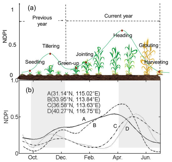
Figure 1.
(a) Normalized differential phenology index (NDPI) [18] curves and the corresponding phenological stages of winter wheat. (b) NDPI curves of winter wheat from different locations in North China. NDPI curves in (a,b) are derived from sentinel-2 MSI data. Curve D is from a location of a rotation of winter wheat and summer corn.
Generally, remote sensing-based methods for winter wheat mapping can be grouped into three types: classification-based methods, index-based methods, and curve similarity-based methods. The first type of method is the classification of one or two satellite images acquired at particular phenology stages, such as at two peak occurrence periods [5,6,7,8,9,10,11]. Unfortunately, the opportunity to acquire high-quality images covering a large area within a specific period is usually limited by long satellite revisit cycles and cloud contamination. Moreover, the collection of a large number of training data covering a large area not only is time consuming, but also has a high field cost. Accordingly, winter wheat mapping over large areas using classification-based methods is not a reasonable solution.
In the second type of method, the VI curve is employed to design specific indices for winter wheat based on its unique phenological features. For example, Pan et al. [8] developed a crop proportion phenology index (CPPI) that used enhanced vegetation index (EVI) values related to the seedling, tillering, heading, and harvesting stages. The CPPI was demonstrated to have a good ability to estimate the winter wheat fraction in a 250 m MODIS pixel through experiments in two small agricultural regions in Beijing and Jiangsu provinces of China. Tao et al. [19] used mathematical transformation to generate the peak before winter feature (PBWF) index associated with the EVI peak amplitude before winter to map winter wheat on the North China Plain, although PBWF neglects the phenological feature variability over large areas. Qiu et al. [14] also proposed two winter wheat indices representing ascending and descending trends before and after the heading date, while ignoring the VI increase before winter. These winter wheat indices typically require prior knowledge of important phenology dates for each pixel due to the large phenological shifts over large areas (see Figure 1b). To address this issue, based on phenological observation data from agrometeorological stations, Qiu et al. [14] built a regression model for the heading date (also the early growing period length) with latitude and altitude, with which the important phenology dates in a specific location can be estimated. Nevertheless, the accuracy of the regression model remains inadequate because the spatial variation in phenology dates is also affected by factors other than latitude and altitude. Meanwhile, such prior knowledge collection or estimation is usually difficult without intensive field surveys or auxiliary data support, which hinders the wide application of this kind of method over large areas [13,15,17].
In the third group of methods, winter wheat is identified by a VI curve similarity measurement without requiring any prior knowledge of important phenology stages. Sun et al. [9] used the Euclidean distance to measure the similarity between any EVI2 curve and a reference EVI2 curve of winter wheat, although the Euclidean distance has limited tolerance for the shifts and distortion of winter wheat curves. Zhang et al. [10] mapped winter wheat in Luoyang city, China with a Kullback–Leibler divergence (KLD)-based method, which was proven effective for land cover classification [20], whereas the KLD classifier lacks verification of winter wheat mapping over larger areas.
Recently, the dynamic time warping (DTW) algorithm, which was originally proposed for speech recognition [21], has also been used in land cover classification [22,23,24,25] due to its ability to tolerate both the shifts and distortions of VI curves. The original DTW identifies the best alignment between two VI curves based on the Euclidean distance without any constraints, which often leads to unreasonable alignment. To address this issue, warping time constraints and a distortion penalty are often imposed to restrict the warping range. For example, Petitjean et al. [26] introduced a constant elapsed time constraint into DTW. Maus et al. [27] proposed time-weighted DTW (TWDTW) with a penalty strategy. The TWDTW method has been successfully utilized for multicrop mapping [28]. Due to the sufficient flexibility of DTW and the considerable efforts devoted to improving DTW performance, the DTW algorithm has been successfully employed for land cover and crop type mapping over large areas [27,28,29,30,31]. Unfortunately, DTW has been applied to winter wheat mapping in only a very limited number of studies [28], possibly due to the more complex characteristics of winter wheat VI curves. The application of DTW to winter wheat mapping over large areas faces the following challenges: (1) how to utilize the special phenological features of winter wheat and (2) how to improve the quality of VI data, especially in the early development stages during which VIs are easily affected by soil background and snow cover.
To address these two challenges, a new curve matching method was developed in this study, termed phenology-time weighted dynamic time warping (PT-DTW), which specifically considers the phenological features of winter wheat. In addition, the normalized differential phenology index (NDPI), also called NDVI+ [18,32], was employed instead of a traditional vegetation index (e.g., NDVI or EVI) to mitigate the effects of the snow and soil background. With the proposed method, winter wheat on the Huang-Huai Plain in North China was mapped at 20 m resolution based on Sentinel 2A/B data, considering the high resolution of Sentinel 2A/B data in both the spatial and temporal dimensions.
2. Materials and Methods
2.1. Study Area and Datasets
The Huang-Huai Plain, located at 29.08°N–42.67°N latitude and 105.18°E–122.70°E longitude (Figure 2), is the largest wheat production zone in China [33] and accounts for 44% of the wheat planting area and 60% of the total wheat production in the country [34]. In this region, there is commonly a rotation between winter wheat and corn/paddy rice, which means that winter wheat is sown after corn/paddy rice harvesting and that corn/paddy rice is planted after the harvesting of winter wheat [2]. Winter wheat is sown in September or October and harvested in May or June of the following year [5]. As the climatic conditions vary widely over the study area, shown by the 2015 annual average air temperature (http://www.resdc.cn/data.aspx?DATAID=228) in Figure 2, there is large intraclass variability in the VI curves of winter wheat in different locations (Figure 1b). In general, the seedling date advances and the heading date is delayed from south to north, leading to a large distortion in the VI curves of winter wheat across the study area. In addition, from north to south, the before-winter peak becomes less obvious due to the higher temperatures in winter in the southern region.
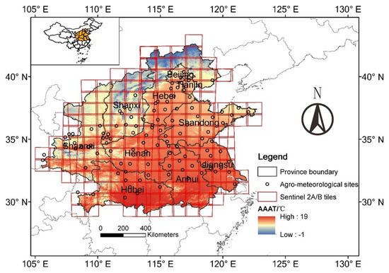
Figure 2.
Study area of Huang-Huai Plain in China. The background raster is annual average air temperature, abbreviated as AAAT.
Sentinel 2 is a European wide-swath, high-resolution, multispectral imaging mission. Two identical satellites (Sentinel 2A/B) provide remotely sensed data with a short revisit cycle (2–3 days at mid-latitudes) and high spatial resolution (10, 20, and 60 m for different spectral bands). A total of 184 tiles of Sentinel 2A/B images cover the entire study area, and all images with less than 80% cloud coverage from September 2017 to June 2018 were downloaded (https://earthexplorer.usgs.gov/). All of the images were used to reconstruct high-quality NDPI curves throughout the growth period of winter wheat (see Section 2.2.1).
The ground truth data were interpreted through high-resolution images acquired at 495 sites in five subregions for winter wheat mapping and accuracy assessment (Figure 3). The layout of these sites was designated along north–south and east–west transects to ensure coverage of multiple agroclimatic zones. The high-resolution images were acquired by an unmanned aerial vehicle system (DJI FC6310) in the growing season of 2017–2018 or Google Earth imagery captured in the winter of 2017. At each sampling site, the corresponding winter wheat patches were visually interpreted using the high-resolution imagery. Then, the interpreted maps were projected to the corresponding 20 m Sentinel pixels (Figure 3). In total, 62,239 ground-truth pixels with 20 m spatial resolution were collected for accuracy evaluation including 27,669 winter wheat and 34,570 other pixels (including forest, barren land, artificial surface, vegetable, paddy rice, water, and grass/shrub land). For the determination of method parameters 80 samples from pure pixels were selected (Section 2.2.3.1), and all the others were used for accuracy assessment. In addition, agricultural census data from 61 municipalities of Beijing, Henan, Anhui, Shandong, Shanxi, Shaanxi, and Anhui in 2017 were acquired from the EPS China Data Platform (http://www.epschinadata.com/). The census data were used to evaluate the overall reliability of the identification of planting areas of winter wheat at the municipal level.
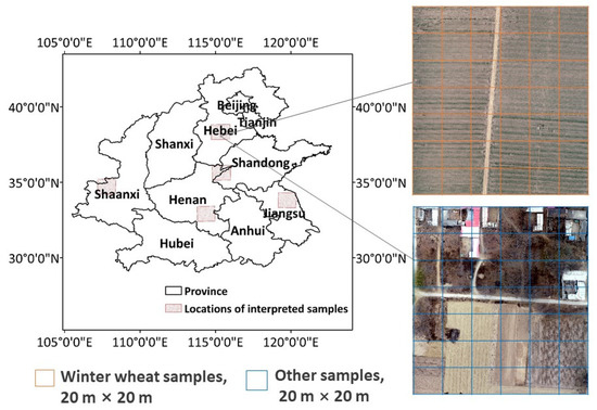
Figure 3.
Samples interpreted using high-resolution imagery.
2.2. Methods
Based on Sentinel 2A/B NDPI time series, we proposed a PT-DTW method for winter wheat mapping in the study area. The workflow consists of the following steps: (a) reconstructing high-quality NDPI time series; (b) optimizing the parameters of the PT-DTW method using simulated samples; and (c) identifying winter wheat and performing accuracy assessment (Figure 4).
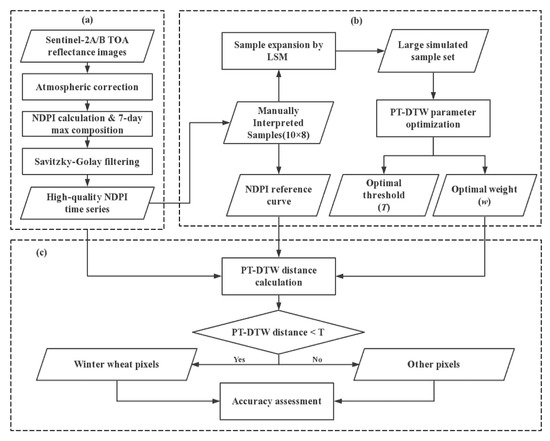
Figure 4.
Workflow of the phenology-time weighted dynamic time warping (PT-DTW) method for winter wheat mapping. (a) Reconstructing high-quality NDPI time series. (b) Optimizing the parameters of the PT-DTW method using simulated samples. (c) Identifying winter wheat and performing accuracy assessment.
2.2.1. Reconstruction of High-quality NDPI Curves
NDPI curves were derived from the multispectral bands of Sentinel 2A/B MSI data in this step. Firstly, the Sentinel 2 data were atmospherically corrected by Sen2Cor (http://step.esa.int/main/third-party-plugins-2/sen2cor/). Secondly, the images of the red (band 4), near-infrared (band 8), and shortwave infrared (band11) bands were all resampled to 20 m spatial resolution, the channel information was listed in Table 1. The NDPI was thus calculated as follows:
where α was set to 0.74, its most effective value for suppressing the variability of the soil and snow backgrounds [18,32]. Thirdly, the NDPI curve was composited with a seven-day maximum composing criterion. We used all of the images with less than 80% cloud contamination, but there was still a lack of observations on some dates and in some areas. To address this issue, the missing observations were linearly interpolated from the valid values on the two nearest dates before and after the missing observations. Finally, Savitzky–Golay filtering for vegetation index reconstruction [35] was performed to reduce the atmospheric effects further and to generate the seven-day NDPI curves at 20 m spatial resolution.

Table 1.
Information of Sentinel 2A/B MSI channels used to calculate NDPI.
2.2.2. Development of the PT-DTW Method
As mentioned before, the phenological features of winter wheat varied widely over large areas (Figure 1b). More specifically, winter wheat is sown later and harvested earlier and thus experiences a shorter growing period from north to south because of the warmer climatic conditions in the south. There is additional and obvious intraclass variation induced by the different growing statuses in winter. In colder areas, winter wheat stops growing and goes dormant in winter and becomes green in early spring. This pattern creates a U-shaped valley in the NDPI curve. Whereas in warmer areas, winter wheat grows continuously through winter and early spring, displaying an insignificant valley in the NDPI curve. These complex features of the NDPI curves may explain why DTW-based methods are not widely used for winter wheat mapping. Fortunately, the winter wheat across the study area also shares common NDPI characteristics in two periods (Figure 5a), i.e., increase before winter and decrease after heading (see the areas with the light yellow background in Figure 5a). These features are not only common features of all winter wheat, but are also distinct from the features of other land cover types. Accordingly, it is still possible to apply the DTW-based method in winter wheat mapping over larger areas if these common phenological features can be enhanced. Therefore, the proposed PT-DTW imposes greater weights on these two important periods when calculating the DTW distance (Figure 5b). The details of the PT-DTW are as follows.
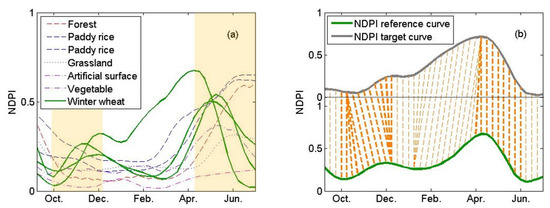
Figure 5.
(a) NDPI curves for different land cover types. Winter wheat shares common characteristics in the two periods with light yellow backgrounds: the NDPI increase before winter and decrease after heading. (b) Phenological weighting strategy of PT-DTW (the thicker dashed line represents greater weight).
Classical DTW Algorithm
The classical DTW algorithm aims to search for optimal alignment of the target and reference curves, which correspond to the warping with the shortest distance between the two curves. Suppose that there are two curves, and , denoting the target and reference curves (Figure 6a), respectively. An m×n matrix (Figure 6a) is constructed to denote the distances between the pairs of elements in the two curves:
where each element in the matrix is defined as . Then, an accumulated distance matrix D is computed by a recursive sum of the minimal distances, such that
with the following initial conditions:
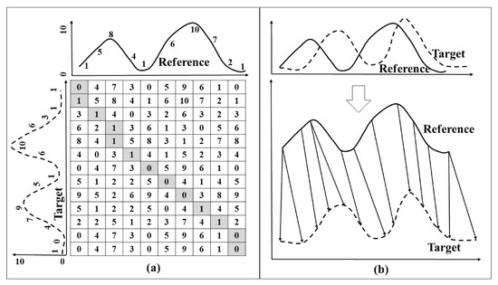
Figure 6.
Illustration of the DTW algorithm. (a) Distance matrix d and warping path P (gray box) computed by DTW. The numbers on the two curves denote the curve magnitudes. Each number in the boxes denotes the difference between the pair of elements in the reference and target curves. (b) Alignment of the two curves determined by DTW.
Then, the warping path in matrix d is determined through the reverse algorithm (Figure 6a). P preserves the indices of the matching elements between the two curves, also called alignment of two curves (Figure 6b). P starts with and ends with . The searching algorithm of P is as follows:
Finally, the shortest warping path P is acquired, and the corresponding DTW distance between U and R is:
where L is the length of P. Equation (3) guarantees the monotonicity and continuity condition [29]. Equations (4) and (6) guarantee that the shortest warping path is restricted to starting with ‘beginning to beginning’ and terminating with ‘ending to ending’.
Logistic Time Penalty
Considering that an excessively large distortion is unreasonable for NDPI curve matching, logistic TWDTW [27] was utilized to avoid the excessively large distortions in classical DTW. A strategy was used that assigns a penalty weight to each element in the distance matrix:
where Mi,j is the penalty weight following a logistic function with midpoint and steepness :
We set α = 0.1 and β = 100 according to the recommendation of Maus et al. [27]. With this penalty on the distance, the unreasonably large distortion of classic DTW can be avoided.
PT-DTW
PT-DTW is specifically designed for winter wheat identification by increasing the importance of the two feature periods and decreasing the impacts of other periods. Specifically, the distances associated with the two feature periods (VI increase before winter and VI decrease after heading) (Figure 5b) were given greater weights, and the other distances were given smaller weights. The phenological weighted function was designed as shown in Equation (9):
where N1 is the total number of alignment associated with the two feature periods of the reference curve; N2 is the total number of alignment associated with the nonfeature periods; ω is the parameter controlling the weight allocation, which was optimized in the simulation experiment (Section 2.2.3); j is the time-phase index in the reference NDPI curve; and Phases 8, 16, 33, and 41 correspond to the NDPI values on 2017/298 (Julian day 298 of the year 2017), 2017/354, 2018/108, and 2018/164, respectively, corresponding to the starting and ending dates of the two feature periods. The timings of the two periods were determined based on the NDPI reference curve of winter wheat (details in Section 2.2.3.1). By combining the phenological weights, the PT-DTW distance between the reference and target curve is:
A smaller PT-DTW distance indicates a higher similarity between the reference and target curve, and winter wheat pixels can be distinguished from others if the distance is less than a certain threshold (T; Equation (11)):
The threshold was also optimized in the simulation experiment (Section 2.2.3).
2.2.3. Determination of PT-DTW Parameters
Several parameters need to be determined for the use of PT-DTW classification, including the NDPI reference curve of winter wheat, phenological weight (ω), and threshold (T). Typically, parameter optimization relies on large training samples. To avoid a large sample collection effort, we designed a simulation experiment to expand the small sample set to a large simulated dataset by using a linear spectral mixing (LSM) model [36,37]. As shown in Figure 4b, 80 manually interpreted samples of different land cover types were firstly collected, one of which was determined to be the reference NDPI curve; then, a large simulated sample set was generated by using a linear mixture model; finally, the parameters ω and T were optimized such that they yielded the highest classification accuracy for the simulated dataset. The details are as follows.
2.2.3.1. Collection of Samples and Determination of the NDPI Reference Curve for Winter Wheat
Based on prior knowledge of the study area, eight land cover types were considered: winter wheat, paddy rice, vegetable, water, artificial surface, forest, grass/shrub land, and barren land. Ten NDPI curves for each land cover type were selected across the study area with reference to high-resolution Google Earth imagery. In total, 80 NDPI curves were selected as initial samples
Regarding the NDPI reference curve, an ideal reference curve should lie in the center of all winter wheat curves. Therefore, the NDPI reference curve for winter wheat was determined as the one with the minimum average Euclidean distance from the nine other winter wheat curves (Figure 7).
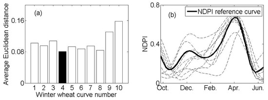
Figure 7.
(a) Average Euclidean distance of each winter wheat NDPI curve from the other curves; Curve No. 4 has the minimum distance (filled-in black bar). (b) NDPI curves of ten winter wheat samples and the reference one.
2.2.3.2. Sample Set Expansion by Using an LSM Model
Considering that the initial sample set, which included only 80 NDPI curves (Figure 8a), was too small to optimize the PT-DTW parameters effectively, the sample set was expanded to a large dataset by using a linear spectral mixing (LSM) model (Figure 8). Mixed NDPI curves were simulated by mixing the NDPI curves of winter wheat endmembers with the NDPI curves of other land cover endmembers. Here, a three-endmember mixture model was considered because it covered most mixing scenarios.
where fwheat is the fraction of wheat endmember, and fnonwheat1 and fnonwheat2 are the fractions of the two nonwheat endmembers. fwheat, fnonwheat1, and fnonwheat2 were generated from the probability density functions shown in Figure 8b. Such distributions guarantee a uniform distribution (0–1) of the wheat fraction and sum-to-one constraint for the three endmembers. Details about the generation process are introduced in the supplementary material. In total, 20,000 mixed NDPI curves were simulated, among which 10,000 were positive samples (fwheat > 50%) and the other 10,000 were negative samples (fwheat < 50%) as shown in Figure 8c.
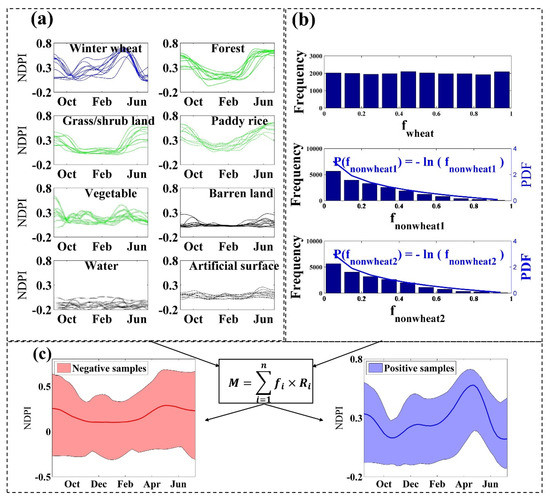
Figure 8.
Sample set expansion by linear spectral mixture model. (a) The 80 NDPI curves of eight endmembers. (b) Probability density functions of endmember fractions. (c) Linear mixing procedure and the 20,000 simulated samples.
2.2.3.3. Parameter Optimization
We varied ω from 0.1 to 1.0 in increments of 0.1 and varied T from the minimum value to the maximum value in 300 steps. Under each ω, the minimum and maximum T are the median PT-DTW distances of the positive and negative samples, respectively. Then, we classified the simulated dataset by using PT-DTW and calculated the overall accuracy with each combination of ω and T (Figure 9). With this optimization procedure, the optimal values of ω = 1 and T = 0.0765, corresponding to the highest overall accuracy (OA; 92.85%), were acquired. As shown in Figure 9b, a large class separability between the positive and negative samples was acquired when ω was equal to 1, indicating that it is a good proxy for distinguishing winter wheat from other land cover types.
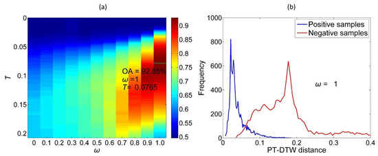
Figure 9.
(a) Optimization of parameters ω and T, where the colors denote the overall accuracies of simulated dataset classification. (b) Class separability between positive and negative samples when ω = 1.
2.2.4. Winter Wheat Mapping and Accuracy Assessment
With the parameters determined above, the PT-DTW distance to the NDPI reference curve of winter wheat was calculated. Finally, the winter wheat pixels in the study area were extracted with the optimal threshold (T = 0.0765). The TWDTW method [27], CBAH method [14], and KLD method [10] were used to map the winter wheat for comparison. The thresholds in the TWDTW, CBAH, and KLD methods were also optimized by performing similar simulation experiments. The overall accuracies and kappa coefficients of these four methods were calculated based on the visually interpreted samples. In addition, the winter wheat areas extracted using the four methods were compared with agricultural census data at the municipal level.
3. Results
3.1. Sentinel 2-Derived Winter Wheat Map for 2017–2018 by PT-DTW Method
Based on Sentinel 2A/B data, a winter wheat map at 20 m resolution was produced using the proposed PT-DTW method. As shown in Figure 10, winter wheat was mainly distributed in Henan and Jiangsu Provinces, Northern Anhui Province, Southern Hebei Province, and Western Shandong Province, which is generally consistent with the results of previous studies [14,18]. The zoomed-in images in Figure 10 show rich spatial details of the winter wheat cropland, and the cultivated parcels are easily recognizable. Considering the fragmented crop cultivation in North China, a 20-m-resolution winter wheat map can provide valuable information for cropland management and policy making.
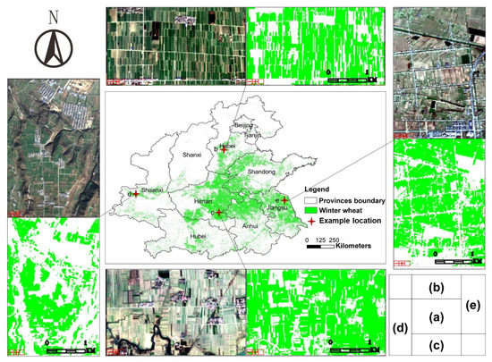
Figure 10.
(a) Winter wheat map of North China in 2017–2018 derived from Sentinel 2 images with the PT-DTW method. (b–e) The sentinel-2 RGB images in December and the zoomed in winter wheat maps of four example locations from Hebei, Henan, Shaanxi and Jiangsu provinces.
3.2. Quantitative Evaluation
The classification accuracies of the PT-DTW, TWDTW, CBAH, and KLD methods were evaluated with 62,239 ground-truth pixels, including 27,669 winter wheat and 34,570 other pixels. Table 2 shows the confusion matrixes and classification accuracy indices of these four methods. The proposed PT-DTW method provides the highest accuracy. The CBAH method also achieves satisfactory accuracy, whereas the TWDTW and KLD methods yield poor classification accuracy.
Table 2.
Accuracy assessment of four methods. Expressed in number of pixels.
The winter wheat pixels derived from Sentinel 2A/B data were aggregated to the municipal level for comparison with the census data, i.e., the municipal-level seeded area of winter wheat in 2017. The cultivated areas of winter wheat estimated using the PT-DTW method matched best with the agricultural census data at the municipal level with a coefficient of determination of 0.8638 and a mean absolute error of 858.8412 km2, although slight overestimation can be found in the municipalities with larger areas of winter wheat (Figure 11a). In contrast, the TWDTW method shows significant overestimation in the municipalities with small areas of winter wheat, and the KLD method shows the largest deviation from the census data. There is also obvious overestimation of the areas estimated by CBAH, especially in the municipalities with small areas of winter wheat, despite good correlations with the census data in other municipalities.
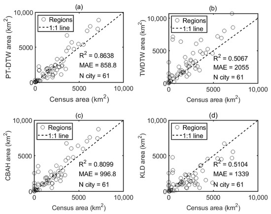
Figure 11.
Municipal-level agreement between agricultural census data and Sentinel 2 estimations of the winter wheat planted areas obtained using the (a) PT-DTW method, (b) proposed time-weighted DTW (TWDTW) method, (c) CBAH method, and (d) KLD method.
3.3. Comparison of Spatial Details
Typical mapping examples of four locations were compared to show the differences among the PT-DTW, CBAH, KLD, and TWDTW methods (Figure 12). In general, the PT-DTW-derived maps show good consistency with the distribution of winter wheat, whereas the other methods produced more classification errors to different degrees. As shown in Figure 12I, II, the KLD-derived winter wheat map is weakly consistent with the spatial pattern of winter wheat patches and has large omission and commission errors. Two shortcomings resulted in the poor performance of the KLD method in winter wheat mapping. Firstly, without reasonable alignment between the target and reference NDPI curves, the KL divergence could not suppress the winter wheat variability across large areas. Secondly, the KLD is a general measure of curve similarity and does not include any consideration of the specific phenology features of winter wheat. The CBAH method is much better for winter wheat mapping. The unique phenological characteristics of winter wheat (i.e., the VI ascending and descending trends before and after heading) are utilized in CBAH classification. However, CBAH overlooks the greenness increase before winter and misclassifies some spring-sown and summer-harvested crops as winter wheat (Figure 12 Ⅲ). Moreover, latitude and altitude are not sufficient to capture all of the variations in sowing and heading date, which are also probably influenced by the local climate and field management. As an example, in Figure 12 Ⅳ, the predicted heading date (DOY 2018113) is earlier than the true heading date (DOY 2018136), leading to some omission error in winter wheat mapping. The TWDTW method, without the consideration of specific phenology periods of winter wheat, yielded poor classification accuracy. TWDTW misclassified forests in mountainous areas (Figure 12 Ⅱ) and spring-sown crops (Figure 12 Ⅲ) as winter wheat and produced salt and pepper noise in the patch of winter wheat cropland (Figure 12 Ⅰ). Compared to the published methods, PT-DTW produced the best winter wheat map due to its effective alignment and its consideration of the specific phenology periods in curve matching.
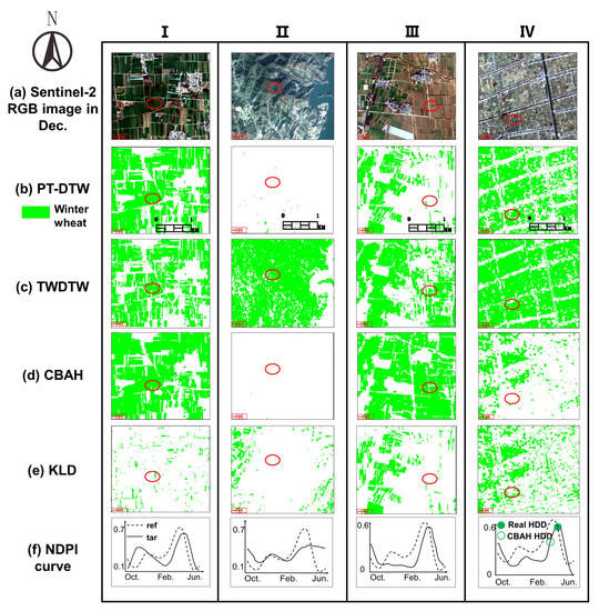
Figure 12.
Comparison of spatial details of four example locations, location Ⅰ (38.6508°N, 115.2872°E), Ⅱ (32.5539°N, 111.0283°E), Ⅲ (37.8897°N, 115.4178°E), and Ⅳ (33.5343°N,120.2 565°E). (a) Sentinel-2 RGB composite images in December. Winter wheat maps derived using the (b) PT-DTW method, (c) TWDTW method, (d) CBAH method, and (e) KLD method. (f) NDPI curves of pixels in the target(tar) regions denoting by red circles and the reference(ref) curve used in PT-DTW method. In the NDPI curve of site Ⅳ, the filled and unfilled green circle indicates the real heading date (Real HDD) and the CBAH method estimated heading date (CBAH HDD).
4. Discussion
4.1. Superiority of NDPI
The NDPI is a newly developed VI that has the advantages of strengthening vegetation information and suppressing soil color variation and snow cover compared to traditional Vis [18,32]. Early growth before winter is the important phenology feature used in PT-DTW to identify winter wheat. However, as winter wheat grows weakly with a low leaf area during that period, traditional VIs may be influenced considerably by the snow and soil background. Therefore, the NDPI was used instead of the NDVI and EVI to capture the weak greenness signal of winter wheat more effectively. To verify whether the NDPI outperforms other VIs in capturing the increase in greenness before winter, the NDPI curves were compared with the NDVI, EVI, and EVI2 curves based on the visually interpreted winter wheat samples. As shown in Figure 13a, the average NDPI curve of winter wheat shows a more obvious increase before winter than the curve of the other VIs. To express the magnitude of the increase quantitatively, a before-winter growth index (BWGI) was calculated for the different VIs:
where is the maximum VI of winter wheat during the winter growing season and is the minimum VI before the winter peak. Specifically, we identified the maximum VI between 01 November 2017 and 31 December 2017 as and the minimum VI between 01 October 2017 and 31 November 2017 as . As shown in Figure 13b, the BWGI of NDPI is significantly larger than those of NDVI, EVI, and EVI2 (p < 0.01 in a t-test), indicating that NDPI captured the winter wheat growth before winter more effectively than NDVI, EVI, and EVI2.
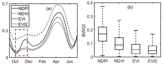
Figure 13.
Comparison of four vegetation index (VI) curves of winter wheat in the period of before-winter growth. (a) Average VI curves of visually interpreted winter wheat pixels. (b) before-winter growth index (BWGI) statistics of the four VIs. The red line and blue box represent the median value and 25th–75th percentiles. The whisker covers the data values within .
4.2. Benefits of the PT-DTW Method
To illustrate the benefits of PT-DTW quantitatively, we further compared the two-class separability, as well as the interclass and intraclass variability, of the PT-DTW, TWDTW, and traditional Euclidean distances of the simulated and visually interpreted samples. All three distances measure the similarity between two curves based on Euclidean distances, while TWDTW and PT-DTW improve the Euclidean distance by including specific curve alignment and phenological feature weighting considerations. To verify the effectiveness of the two abovementioned enhancements, the two-class separability is defined as follows [38,39]:
where and are the mean values for the winter wheat and other samples, respectively; denotes the interclass variability; and and are the standard deviations of winter wheat and other land cover types, denoting the intraclass variability. As shown in Figure 14, the PT-DTW distance produces the most distinctive histograms between winter wheat and other land cover types among the three distances, followed by the TWDTW and Euclidean distances. Table 3 provides more detailed information about the two-class separability, interclass variability, and intraclass variability. The TWDTW and PT-DTW distances show much smaller intraclass variability of winter wheat than the Euclidean distance (Table 3), indicating that DTW-based alignment can effectively tolerate the shifts and distortions of the NDPI curves of winter wheat. Despite its effectiveness in suppressing the intraclass variability of winter wheat, the classification accuracy of TWDTW is only slightly higher than that of the Euclidean distance, because the interclass variability is also reduced. With the optimization of phenology weighting, PT-DTW greatly increased the interclass variability while simultaneously maintaining low intraclass variability (Table 3), suggesting that weighting on certain phenology periods successfully enhanced the distinctive features of winter wheat. In summary, the above results confirmed the effectiveness of TWDTW alignment and phenology weighting in extracting winter wheat with PT-DTW.
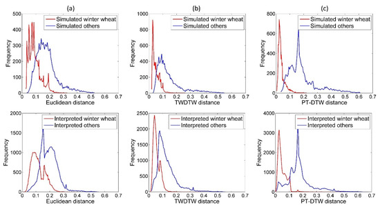
Figure 14.
(a) Euclidean distance, (b) TWDTW distance, and (c) PT-DTW distance of simulated and visually interpreted winter wheat and other samples.
Table 3.
Comparison of Euclidean distance-based methods through simulated and field samples.
4.3. Transferability of PT-DTW Method
Winter wheat phenology is dominated by climatic factors and field management. Thus, the phenology shifts appear not only over large areas, but also across different years. To validate whether the PT-DTW method can be applied to other years, one tile of the Sentinel 2 (50SLH) NDPI time series from 2018-2019 was used to derive the winter wheat map through PT-DTW with the same parameters employed in the 2017–2018 mapping. The winter wheat cultivation in this area located in Hebei province, experienced some changes because of the new crop rotation and fallow policy implemented since 2016 [40,41]. As shown in Figure 15, the transitions between the winter wheat and fallow land were successfully detected by the PT-DTW method without retraining the PT-DTW parameters. The land cover types of 3786 cloud-free pixels were interpreted visually through images acquired in 2017/12/24 and 2018/12/09, considering that winter wheat shows greenness within cropland in winter. The change detection accuracy was then evaluated, as shown in Table 4. An OA of 93.66% in change detection indicates the great potential of PT-DTW for rapid winter wheat mapping in multiple years. Although some of the published methods, such as CBAH, can achieve comparable accuracy with the support of auxiliary data, as mentioned in Section 3.2 and Section 3.3, the PT-DTW method is proven to be more flexible and practical, given the lower demand for auxiliary data and great temporal transferability.
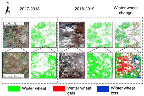
Figure 15.
Sentinel-2 RGB images acquired on 24 December 2017 and 09 December 2018, PT-DTW-derived winter wheat maps of 2017–2018 and 2018–2019, and changes of winter wheat planting in the area covered by tile 50SLH of Sentinel-2 images.
Table 4.
Winter wheat change detection accuracy assessment. Expressed in number of pixels.
In addition to the temporal transferability of winter wheat mapping, the proposed PT-DTW has the potential to be modified for mapping other crops besides winter wheat. Although PT-DTW cannot be directly used to map other crops because the parameters were specifically determined based on the phenological features of winter wheat, it would not be difficult to set up a new group of parameters to classify other crops using a strategy similar to that employed in this study. If key phenological stages could be determined based on prior knowledge, the parameters could also be trained through a small number of field samples using the method described in Section 2.2.3. After the parameters were redetermined, the retrained PT-DTW could be used to classify other crops.
4.4. Influence of Cloud Contamination
Cloud contamination is a considerable obstacle for time-series matching. Thus, a simulation experiment was conducted to explore the sensitivity of the PT-DTW method to cloud contamination. First, all the visually interpreted samples with little cloud contamination were selected as the benchmark data for analysis. Second, cloudy NDPI curves were simulated by randomly replacing the clear observations with cloudy ones (NDPI was set to 0). The different cloud percentages and different fractions of cloud observations in key phenological stages in the total cloud observations were considered (details in the Supplementary Material). Finally, the simulated cloudy NDPI time-series were used to classify winter wheat, by PT-DTW with the same time series reconstruction procedure (Section 2.2.1) and parameters. As shown in Figure 16a, the OA decreases marginally when the cloud percentage is less than 50%, indicating that the Savizky–Golay filter performed well in reconstructing the NDPI time series. Figure 16b shows that the uneven cloud distributions in key and nonkey phenological stages also marginally affect the classification accuracy when the cloud percentage is less than 50%, which may be because the overall NDPI curve shape did not change considerably regardless of how the cloud observations were distributed in key and nonkey phenological stages. The above results indicate that the PT-DTW method is suitable for winter wheat mapping when the percentage of clear Sentinel 2 observations is greater than 50% throughout the growing period of winter wheat.
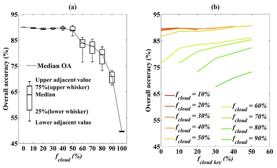
Figure 16.
Sensitivity of the PT-DTW method to the percentage of cloud observations in the whole growing period (a) and in the key phenological stage (b). fcloud and fcloud key denote the fractions of cloud observations in the whole growing period and in the key phenological stage. The black box plot in (a) represents the range of OA variation with uneven distributions of cloud observations in key and nonkey stages.
4.5. Limitations of the PT-DTW Method
Several limitations remain in the proposed PT-DTW method. Firstly, the Euclidean distance is calculated to measure the difference between the target and reference curves, leading to a relatively high sensitivity to the magnitude variability of NDPI curves. Thus, winter wheat pixels with poor growth status are likely to be misclassified due to their lower NDPI values. Induction of the distances into non-Euclidean space is a possible solution; however, this approach would increase the mathematical complexity of the algorithms. The data quality may also affect the mapping accuracy. As mentioned in the previous section, PT-DTW performs poorly when the cloud percentage of Sentinel 2 data is greater than 50%, which could occur in Southern China. The fusion of cloud-free SAR data could provide VI time-series data with better quality and help improve the performance of wheat mapping [42].
5. Conclusions
In this study, a PT-DTW method was proposed for winter wheat mapping over a large area based on the NDPI curves derived from Sentinel 2A/B data. With specific improvements over the classical DTW and TWDTW, PT-DTW can tolerate the variability of VI curves of winter wheat over large areas and works well without considerable sampling effort. Comparison experiments showed that the PT-DTW method outperforms previous methods, achieves reasonable mapping accuracy, and is transferable to winter wheat mapping in different years. Therefore, the PT-DTW method is recommended for winter wheat mapping over large areas and in multiple years, requiring only a small number of samples for parameter training.
With the proposed PT-DTW, the winter wheat of North China in 2017–2018 was mapped at 20 m resolution, which is the highest resolution in a winter wheat map of this area to our knowledge. The map produced at this spatial resolution can provide rich spatial details for the area, which has fragmented crop cultivation.
Supplementary Materials
The following are available online at https://www.mdpi.com/2072-4292/12/8/1274/s1.
Author Contributions
Conceptualization, Q.D., X.C. (Xuehong Chen) and J.C.; methodology, Q.D., J.C. and C.Z.; software, Q.D., X.C. (Xuehong Chen), C.Z. and L.L.; formal analysis, Q.D. and Y.Z.; investigation, X.C. (Xin Cao), X.Z., and X.C. (Xihong Cui); writing—original draft preparation, Q.D. and X.C. (Xuehong Chen); writing—review and editing, J.C. All authors have read and agreed to the published version of the manuscript.
Funding
This work was funded by the National Key Research and Development Program of China (No. 2017YFD0300201) and the Science and Technology Facilities Council of UK- Newton Agritech Program (Sentinels of Wheat).
Conflicts of Interest
The authors declare no conflict of interest.
References
- Shiferaw, B.; Smale, M.; Braun, H.-J.; Duveiller, E.; Reynolds, M.; Muricho, G. Crops that feed the world 10. Past successes and future challenges to the role played by wheat in global food security. Food Secur. 2013, 5, 291–317. [Google Scholar] [CrossRef]
- Jin, S. Wheat in China; China Agricultural Press: Beijing, China, 1996; pp. 2–5. [Google Scholar]
- Fan, L.; Liang, S.; Chen, H.; Hu, Y.; Zhang, X.; Liu, Z.; Wu, W.; Yang, P. Spatio-temporal analysis of the geographical centroids for three major crops in China from 1949 to 2014. J. Geogr. Sci. 2018, 28, 1672–1684. [Google Scholar] [CrossRef]
- Wang, X.; Li, X.; Tan, M.; Xin, L. Remote sensing monitoring of changes in winter wheat area in North China Plain from 2001 to 2011. Trans. Chin. Soc. Agric. Eng. 2015, 31, 190–199. [Google Scholar]
- Jia, K.; Wu, B.; Li, Q. Crop classification using HJ satellite multispectral data in the North China Plain. J. Appl. Remote Sens. 2013, 7, 573–576. [Google Scholar] [CrossRef]
- Chu, L.; Liu, Q.-S.; Huang, C.; Liu, G.-H. Monitoring of winter wheat distribution and phenological phases based on MODIS time-series: A case study in the Yellow River Delta, China. J. Integr. Agric. 2016, 15, 2403–2416. [Google Scholar] [CrossRef]
- Liang, Y.; Wan, J. Application of HJ-1A/B-CCD Images in Extracting the Distribution of Winter Wheat and Rape in Hubei Province. Chin. J. Agrometeorol. 2012, 33, 573–578. [Google Scholar]
- Pan, Y.; Li, L.; Zhang, J.; Liang, S.; Zhu, X.; Sulla-Menashe, D. Winter wheat area estimation from MODIS-EVI time series data using the Crop Proportion Phenology Index. Remote Sens. Environ. 2012, 119, 232–242. [Google Scholar] [CrossRef]
- Sun, H.; Xu, A.; Lin, H.; Zhang, L.; Mei, Y. Winter wheat mapping using temporal signatures of MODIS vegetation index data. Int. J. Remote Sens. 2012, 33, 5026–5042. [Google Scholar] [CrossRef]
- Zhang, X.; Qiu, F.; Qin, F. Identification and mapping of winter wheat by integrating temporal change information and Kullback–Leibler divergence. Int. J. Appl. Earth Obs. Geoinf. 2019, 76, 26–39. [Google Scholar] [CrossRef]
- Zhu, S.; Zhang, J.; Shuai, G.; Yu, Q. Winter wheat mapping by soft and hard land use/cover change detection. J. Remote. Sens. 2014, 18, 476–496. [Google Scholar]
- Li, L.; Zhang, J.-S.; Zhu, W.-Q.; Hu, T.-G.; Hou, D. Winter Wheat Area Estimation with MODIS-NDVI Time Series Based on Parcel. Guang Pu Xue Yu Guang Pu Fen Xi 2011, 31, 1379–1383. [Google Scholar]
- Foerster, S.; Kaden, K.; Foerster, M.; Itzerott, S. Crop type mapping using spectral–temporal profiles and phenological information. Comput. Electron. Agric. 2012, 89, 30–40. [Google Scholar] [CrossRef]
- Qiu, B.; Luo, Y.; Tang, Z.; Chen, C.; Lu, D.; Huang, H.; Chen, Y.; Chen, N.; Xu, W. Winter wheat mapping combining variations before and after estimated heading dates. ISPRS-J. Photogramm. Remote Sens. 2017, 123, 35–46. [Google Scholar] [CrossRef]
- Siebert, S.; Ewert, F. Spatio-temporal patterns of phenological development in Germany in relation to temperature and day length. Agric. For. Meteorol. 2012, 152, 44–57. [Google Scholar] [CrossRef]
- Wardlow, B.D.; Egbert, S.L. Large-area crop mapping using time-series MODIS 250 m NDVI data: An assessment for the U.S. Central Great Plains. Remote Sens. Environ. 2008, 112, 1096–1116. [Google Scholar] [CrossRef]
- Wardlow, B.; Egbert, S.; Kastens, J. Analysis of Time-Series MODIS 250 m Vegetation Index Data for Crop Classification in the U.S. Central Great Plains. Remote Sens. Environ. 2007, 108, 290–310. [Google Scholar] [CrossRef]
- Wang, C.; Chen, J.; Wu, J.; Tang, Y.; Shi, P.; Black, T.A.; Zhu, K. A snow-free vegetation index for improved monitoring of vegetation spring green-up date in deciduous ecosystems. Remote Sens. Environ. 2017, 196, 1–12. [Google Scholar] [CrossRef]
- Tao, J.-b.; Wu, W.-b.; Zhou, Y.; Wang, Y.; Jiang, Y. Mapping winter wheat using phenological feature of peak before winter on the North China Plain based on time-series MODIS data. J. Integr. Agric. 2017, 16, 348–359. [Google Scholar] [CrossRef]
- Zhou, Y.; Qiu, F. Fusion of high spatial resolution WorldView-2 imagery and LiDAR pseudo-waveform for object-based image analysis. ISPRS-J. Photogramm. Remote Sens. 2015, 101, 221–232. [Google Scholar] [CrossRef]
- Sakoe, H.; Chiba, S. Dynamic-programming algorithm optimization for spoken word recognition. IEEE Trans. Signal Process. 1978, 26, 43–49. [Google Scholar] [CrossRef]
- Costa, W.S.; Fonseca, L.M.G.; Körting, T.S.; Bendini, H.d.N.; Souza, R.C.M.d. Spatio-Temporal Segmentation Applied to Optical Remote Sensing Image Time Series. IEEE Geosci. Remote. Sens. Lett. 2018, 15, 1299–1303. [Google Scholar] [CrossRef]
- Petitjean, F.; Inglada, J.; Gancarski, P. Satellite Image Time Series Analysis under Time Warping. IEEE Trans. Geosci. Remote. Sens. 2012, 50, 3081–3095. [Google Scholar] [CrossRef]
- Weber, J.; Petitjean, F.; Ganarski, P. Towards efficient satellite image time series analysis: Combination of dynamic time warping and quasi-flat zones. In Proceedings of the 2012 IEEE International Geoscience and Remote Sensing Symposium, Munich, Germany, 22–27 July 2012; pp. 4387–4390. [Google Scholar] [CrossRef]
- Xue, Z.; Du, P.; Feng, L. Phenology-Driven Land Cover Classification and Trend Analysis Based on Long-term Remote Sensing Image Series. IEEE J. Sel. Top. Appl. Earth Observ. Remote Sens. 2014, 7, 1142–1156. [Google Scholar] [CrossRef]
- Petitjean, F.; Inglada, J.; Gancarski, P. Introducing prior knowledge in temporal distances for Satellite Image Time Series analysis. In Proceedings of the 2012 IEEE International Geoscience and Remote Sensing Symposium, Munich, Germany, 22–27 July 2012; pp. 5426–5429. [Google Scholar] [CrossRef]
- Maus, V.; Câmara, G.; Souza, R.; Sanchez, A.; Ramos, F.; Queiroz, G. A Time-Weighted Dynamic Time Warping Method for Land-Use and Land-Cover Mapping. IEEE J. Sel. Top. Appl. Earth Observ. Remote Sens. 2016, 9, 3729–3739. [Google Scholar] [CrossRef]
- Belgiu, M.; Csillik, O. Sentinel-2 cropland mapping using pixel-based and object-based time-weighted dynamic time warping analysis. Remote Sens. Environ. 2018, 204, 509–523. [Google Scholar] [CrossRef]
- Guan, X.; Huang, C.; Liu, G.; Meng, X.; Liu, Q. Mapping Rice Cropping Systems in Vietnam Using an NDVI-Based Time-Series Similarity Measurement Based on DTW Distance. Remote Sens. 2016, 8, 19. [Google Scholar] [CrossRef]
- Maus, V.; Câmara, G.; Cartaxo, R.; Ramos, F.M.; Sanchez, A.; Ribeiro, G.Q. Open boundary dynamic time warping for satellite image time series classification. In Proceedings of the 2015 IEEE International Geoscience and Remote Sensing Symposium (IGARSS), Milan, Italy, 26–31 July 2015; pp. 3349–3352. [Google Scholar]
- Petitjean, F.; Puissant, A.; Gancarski, P. Monitoring urban sprawl from satellite image time series. In Proceedings of the 2012 IEEE International Geoscience and Remote Sensing Symposium, Munich, Germany, 22–27 July 2012; pp. 5963–5966. [Google Scholar] [CrossRef]
- Chen, X.; Guo, Z.; Chen, J.; Yang, W.; Yao, Y.; Zhang, C.; Cui, X.; Cao, X. Replacing the Red Band with the Red-SWIR Band (0.74ρred+0.26ρswir) Can Reduce the Sensitivity of Vegetation Indices to Soil Background. Remote Sens. 2019, 11, 851. [Google Scholar] [CrossRef]
- Ren, J.; Chen, Z.; Zhou, Q.; Tang, H. Regional yield estimation for winter wheat with MODIS-NDVI data in Shandong, China. Int. J. Appl. Earth. Obs. Geoinf. 2008, 10, 403–413. [Google Scholar] [CrossRef]
- Yu, Z.; Tian, Q.; Pan, Q.; Yue, S.; Wang, D.; Duan, Z.; Duan, L.; Wang, Z.; Niu, Y. Theory and Practice on Cultivation of Super High Yield of Winter Wheat in the Wheat Fields of Yellow River and Huaihe River Districts. Zuo Wu Xue Bao 2002, 28, 577–585. [Google Scholar]
- Chen, J.; Jönsson, P.; Tamura, M.; Gu, Z.; Matsushita, B.; Eklundh, L. A simple method for reconstructing a high-quality NDVI time-series data set based on the Savitzky–Golay filter. Remote Sens. Environ. 2004, 91, 332–344. [Google Scholar] [CrossRef]
- Chen, J.; Yuan Zhang, M.; Wang, L.; Shimazaki, H.; Tamura, M. A new index for mapping lichen-dominated biological soil crusts in desert areas. Remote Sens. Environ. 2005, 96, 165–175. [Google Scholar] [CrossRef]
- Roberts, D.A.; Gardner, M.; Church, R.; Ustin, S.; Scheer, G.; Green, R.O. Mapping chaparral in the Santa Monica Mountains using multiple endmember spectral mixture models. Remote Sens. Environ. 1998, 65, 267–279. [Google Scholar] [CrossRef]
- Guo, Z.; Yang, D.; Chen, J.; Cui, X. A new index for mapping the ‘blue steel tile’ roof dominated industrial zone from Landsat imagery. Remote Sens. Lett. 2018, 9, 578–586. [Google Scholar] [CrossRef]
- Kaufman, Y.J.; Remer, L.A. Detection of forests using mid-nir reflectance—An application for aerosol studies. IEEE Trans. Geosci. Remote Sens. 1994, 32, 672–683. [Google Scholar] [CrossRef]
- The Implementation Plan of Agricultural Project for Comprehensive Management of Groundwater Overexploitation in Hebei Province; Department of Agriculture and Rural Affairs of Hebei Province: Shijiazhuang, China, 2016.
- The Implementation Plan of Hebei Province’s Seasonal Fallow System in 2016; Department of Agriculture and Rural Affairs of Hebei Province: Shijiazhuang, China, 2016.
- Song, Y.; Wang, J. Mapping Winter Wheat Planting Area and Monitoring Its Phenology Using Sentinel-1 Backscatter Time Series. Remote Sens. 2019, 11, 449. [Google Scholar] [CrossRef]


© 2020 by the authors. Licensee MDPI, Basel, Switzerland. This article is an open access article distributed under the terms and conditions of the Creative Commons Attribution (CC BY) license (http://creativecommons.org/licenses/by/4.0/).