Improved Inference and Prediction for Imbalanced Binary Big Data Using Case-Control Sampling: A Case Study on Deforestation in the Amazon Region


Abstract

1. Introduction
2. Materials and Methods
2.1. Case-Control Sampling
2.1.1. Inference from Case-Control Data
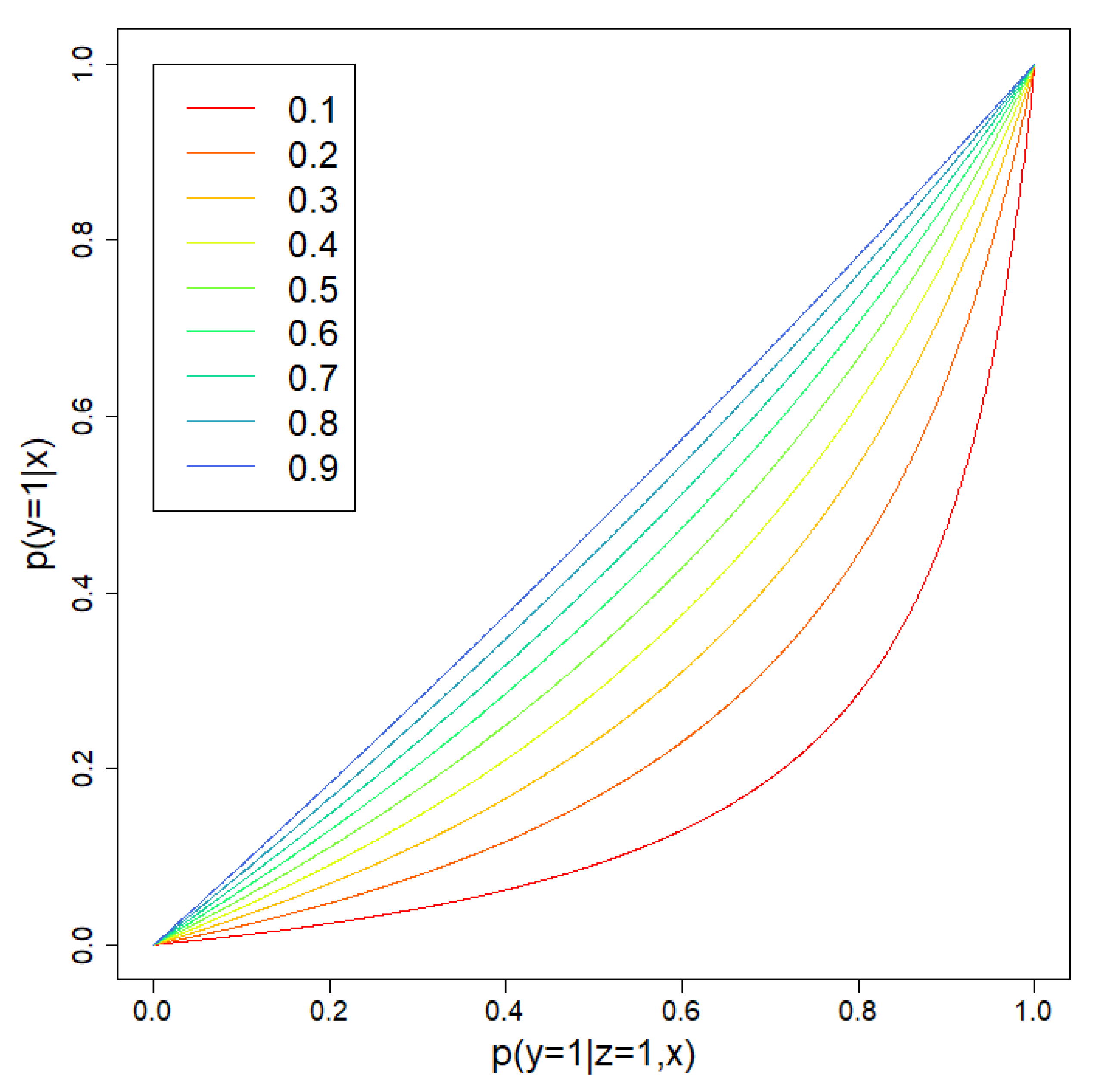
2.1.2. Prediction Based on Case-Control Data
2.2. Simulations
2.3. Case Study on Deforestation in the Amazon Region
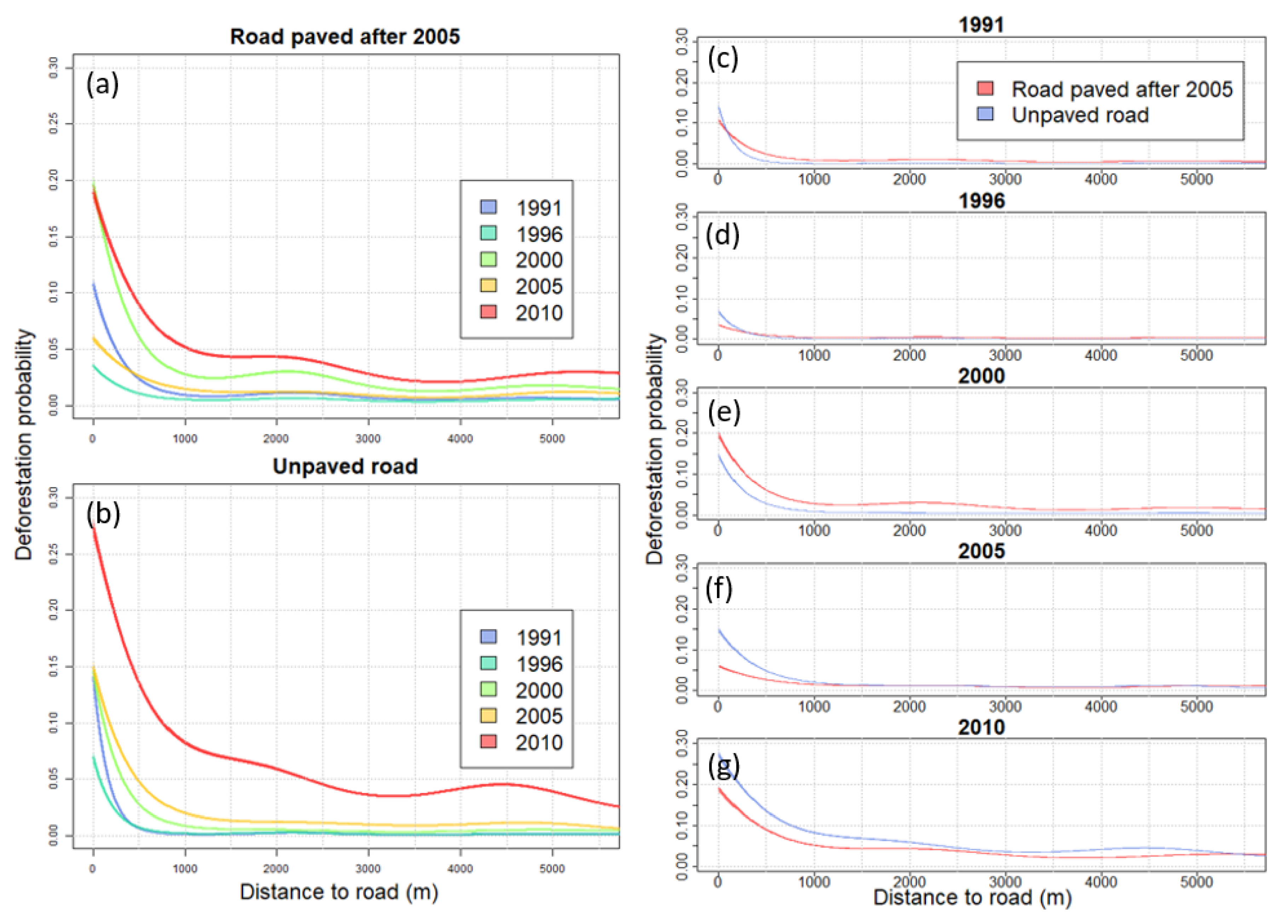
2.3.1. Inference on the Effect of Road Proximity and Road Paving on Deforestation Risk
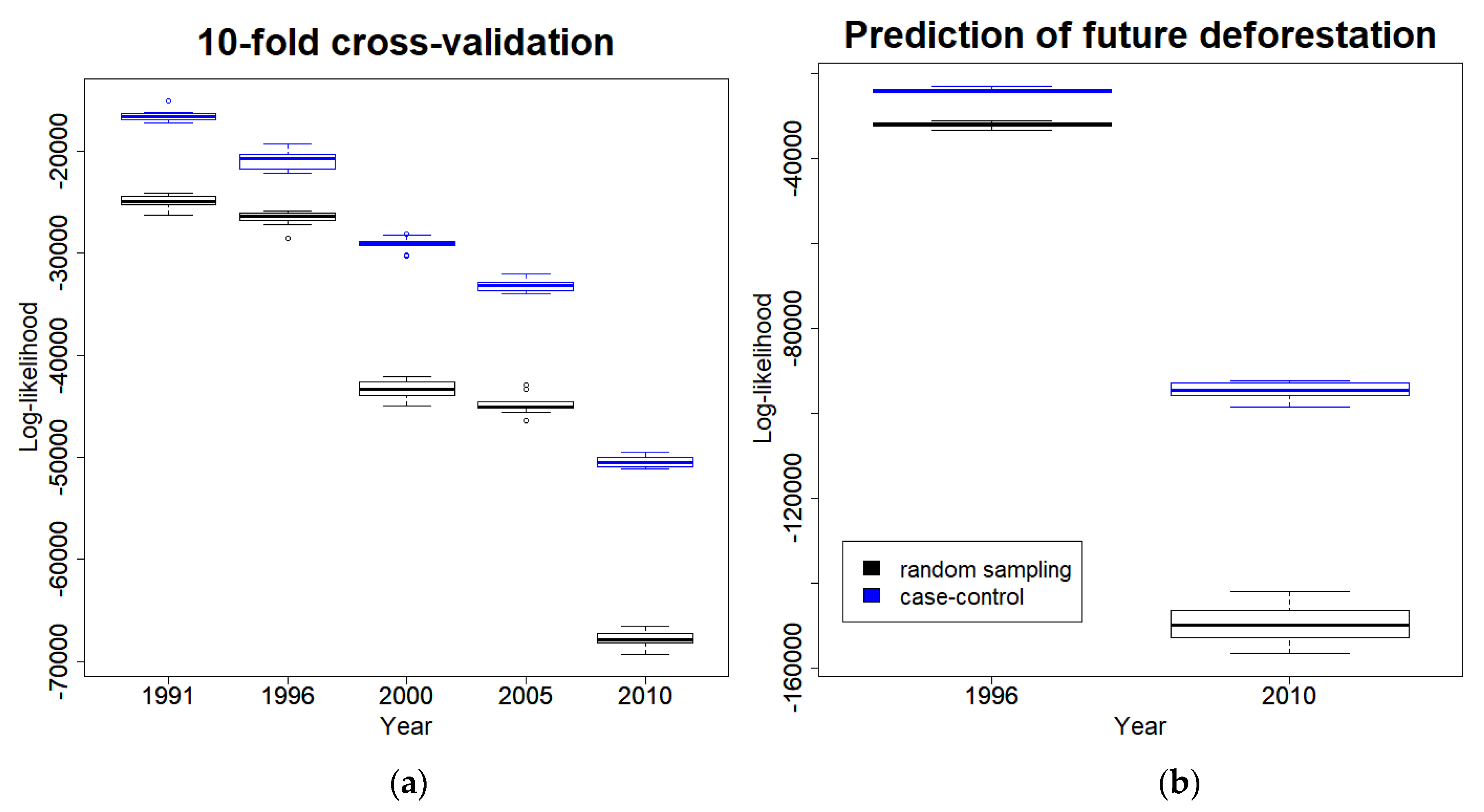
2.3.2. Predicting Deforestation Risk
3. Results
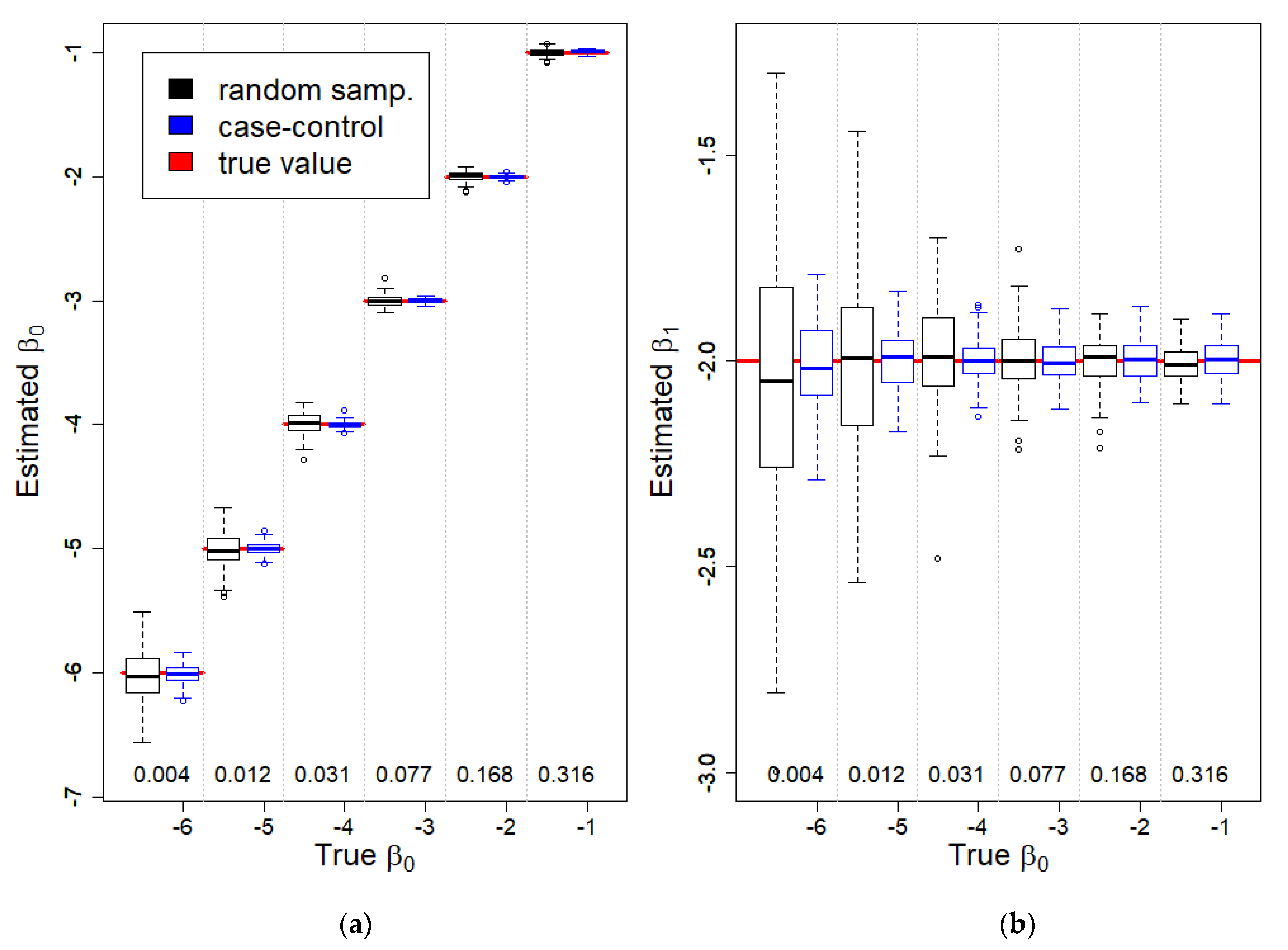
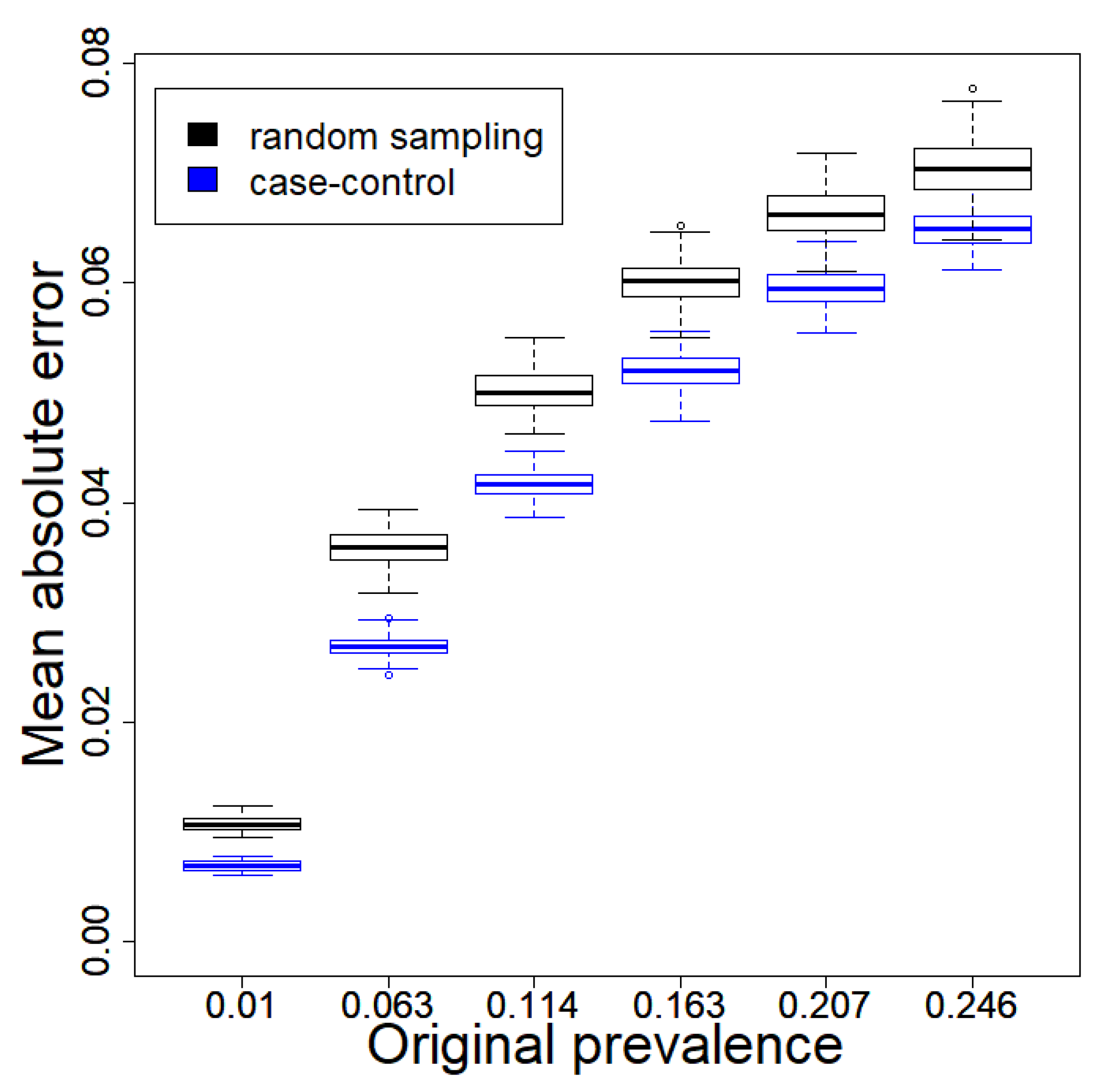
3.1. Simulations
3.2. Case study on Deforestation in the Amazon Region
3.2.1. Modeling the Effect of Proximity to Road and the Effect of Road Paving on Deforestation Risk
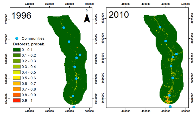
3.2.2. Predicting Deforestation Risk
4. Discussion
5. Conclusions
Author Contributions
Funding
Acknowledgments
Conflicts of Interest
References
- Bakker, D.C.E.; Pfeil, B.; Landa, C.S.; Metzl, N.; O’Brien, K.M.; Olsen, A.; Smith, K.; Cosca, C.; Harasawa, S.; Jones, S.D.; et al. A multi-decade record of high-quality fCO2 data in version 3 of the Surface Ocean CO2 Atlas (SOCAT). Earth Syst. Sci. Data 2016, 8, 383–413. [Google Scholar] [CrossRef]
- Richardson, A.D.; Hufkens, K.; Milliman, T.; Aubrecht, D.M.; Chen, M.; Gray, J.M.; Johnston, M.R.; Keenan, T.F.; Klosterman, S.T.; Kosmala, M.; et al. Tracking vegetation phenology across diverse North American biomes using PhenoCam imagery. Sci. Data 2018, 5, 180028. [Google Scholar] [CrossRef]
- WCS. A New Cloud Platform Unveils the Most Diverse Camera Trap Database in the World. Available online: https://newsroom.wcs.org/News-Releases/articleType/ArticleView/articleId/13593/A-New-Cloud-Platform-Unveils-the-Most-Diverse-Camera-Trap-Database-in-the-World.aspx (accessed on 6 February 2020).
- Wulder, M.A.; Loveland, T.R.; Roy, D.P.; Crawford, C.J.; Masek, J.G.; Woodcock, C.E.; Allen, R.G.; Anderson, M.C.; Belward, A.S.; Cohen, W.B.; et al. Current status of Landsat program, science, and applications. Remote. Sens. Environ. 2019, 225, 127–147. [Google Scholar] [CrossRef]
- Zhou, Y.; Smith, S.J.; Zhao, K.; Imhoff, M.; Thomson, A.; Bond-Lamberty, B.; Asrar, G.R.; Zhang, X.; He, C.; Elvidge, C.D. A global map of urban extent from nightlights. Environ. Res. Lett. 2015, 10, 054011. [Google Scholar] [CrossRef]
- Asner, G.P.; Knapp, D.E.; Broadbent, E.N.; Oliveira, P.J.C.; Keller, M.; Silva, J.N. Selective logging in the Brazilian Amazon. Science 2005, 310, 480–482. [Google Scholar] [CrossRef] [PubMed]
- Pekel, J.-F.; Cottam, A.; Gorelick, N.; Belward, A.S. High-resolution mapping of global surface water and its long-term changes. Nature 2016, 540, 418–422. [Google Scholar] [CrossRef] [PubMed]
- Parkinson, C.L. A 40-y record reveals gradual Antarctic sea ice increases followed by decreases at rates far exceeding the rates seen in the Artic. Proc. Natl. Acad. Sci. USA 2019, 116, 14414–14423. [Google Scholar] [CrossRef] [PubMed]
- Bunting, P.; Rosenqvist, A.; Lucas, R.M.; Rebelo, L.-M.; Hilarides, L.; Thomas, N.; Hardy, A.; Itoh, T.; Shimada, M.; Finlayson, C.M. The global mangrove watch—A new 2010 global baseline of mangrove extent. Remote Sens. 2019, 10, 1669. [Google Scholar] [CrossRef]
- Southgate, D.; Sierra, R.; Brown, L. The causes of tropical deforestation in Ecuador: A statistical analysis. World Dev. 1991, 19, 1145–1151. [Google Scholar] [CrossRef]
- Pfaff, A.S.P. What drivers deforestation in the Brazilian Amazon? J. Environ. Econ. Manag. 1999, 37, 26–43. [Google Scholar] [CrossRef]
- Jusys, T. Fundamental causes and spatial heterogeneity of deforestation in Legal Amazon. Appl. Geogr. 2016, 75, 188–199. [Google Scholar] [CrossRef]
- Soares-Filho, B.S.; Nepstad, D.; Curran, L.M.; Cerqueira, G.C.; Garcia, R.A.; Ramos, C.A.; Voll, E.; McDonald, A.; Lefebvre, P.; Schlesinger, P. Modelling conservation in the Amazon basin. Nature 2006, 440, 520–523. [Google Scholar] [CrossRef] [PubMed]
- Aguiar, A.P.D.; Camara, G.; Escada, M.I.S. Spatial statistical analysis of land-use determinants in the Brazilian Amazonia: Exploring intra-regional heterogeneity. Ecol. Model. 2007, 209, 169–188. [Google Scholar] [CrossRef]
- Laurance, W.F.; Albernaz, A.K.M.; Schroth, G.; Fearnside, P.M.; Bergen, S.; Venticinque, E.M.; da Costa, C. Predictors of deforestation in the Brazilian Amazon. J. Biogeogr. 2002, 29, 737–748. [Google Scholar] [CrossRef]
- Chomitz, K.M.; Gray, D.A. Roads, land use, and deforestation: A spatial model applied to Belize. World Bank Econ. Rev. 1996, 10, 487–512. [Google Scholar] [CrossRef]
- Ludeke, A.K.; Maggio, R.C.; Reid, L.M. An analysis of anthropogenic deforestation using logistc regression and GIS. J. Environ. Manag. 1990, 31, 247–259. [Google Scholar] [CrossRef]
- Green, J.M.H.; Larrosa, C.; Burgess, N.D.; Balmford, A.; Johnston, A.; Mbilinyi, B.P.; Platts, P.J.; Coad, L. Deforestation in an African biodiversity hotspot: Extent, variation and the effectiveness of protected areas. Biol. Conserv. 2013, 164, 62–72. [Google Scholar] [CrossRef]
- Barber, C.P.; Cochrane, M.A.; Souza, C.M., Jr.; Laurance, W.F. Roads, deforestation, and the mitigating effect of protected areas in the Amazon. Biol. Conserv. 2014, 177, 203–209. [Google Scholar] [CrossRef]
- Southworth, J.; Marsik, M.; Qiu, Y.; Perz, S.; Cumming, G.; Stevens, F.; Rocha, K.; Duchelle, A.; Barnes, G. Roads as drivers of change: Trajectories across the tri-national frontier in MAP, the southwestern Amazon. Remote Sens. 2011, 3, 1047–1066. [Google Scholar] [CrossRef]
- Sales, M.; de Bruin, S.; Herold, M.; Kyriakidis, P.; Souza, C., Jr. A spatiotemporal geostatistical hurdle model approach for short-term deforestation prediction. Spat. Stat. 2017, 21, 304–318. [Google Scholar] [CrossRef]
- Mertens, B.; Poccard-Chapuis, R.; Piketty, M.-G.; Lacques, A.-E.; Venturieri, A. Crossing spatial analyses and livestock economics to understand deforestation processes in the Brazilian Amazon: The case of Sao Felix do Xingu in south Para. Agric. Econ. 2002, 27, 269–294. [Google Scholar]
- Echeverria, C.; Coomes, D.A.; Hall, M.; Newton, A.C. Spatially explicit models to analyze forest loss and fragmentation between 1976 and 2020 in southern Chile. Ecol. Model. 2008, 212, 439–449. [Google Scholar] [CrossRef]
- Cushman, S.A.; Macdonald, E.A.; Landguth, E.L.; Malhi, Y.; Macdonald, D.W. Multiple-scale prediction of forest loss risk across Borneo. Landsc. Ecol. 2017, 32, 1581–1598. [Google Scholar] [CrossRef]
- Voight, C.; Hernandez-Aguilar, K.; Garcia, C.; Gutierrez, S. Predictive modeling of future forest cover change patterns in southern Belize. Remote Sens. 2019, 11, 823. [Google Scholar] [CrossRef]
- Pijanowski, B.C.; Tayyebi, A.; Doucette, J.; Pekin, B.K.; Braun, D.; Plourde, J. A big data urban growth simulation at a national scale: Configuring the GIS and neural network based Land Transformation Model to run in a High Performance Computing (HPC) environment. Environ. Model. Softw. 2014, 51, 250–268. [Google Scholar] [CrossRef]
- Kuhn, M.; Johnson, K. Chapter 16. Remedies for Severe Class Imbalance. In Applied Predictive Modeling; Springer: New York, NY, USA, 2016. [Google Scholar]
- Van Hulse, J.; Khoshgoftaar, T.M.; Napolitano, A. Experimental perspectives on learning from imbalanced data. In Proceedings of the 24th International Conference on Machine Learning, Corvallis, OR, USA, 20–24 June 2007; pp. 935–942. [Google Scholar]
- Lemaitre, G.; Nogueira, F.; Aridas, C.K. Imbalanced-learn: A Python toolbox to tackle the curse of imbalanced datasets in machine learning. J. Mach. Learn. Res. 2017, 18, 1–5. [Google Scholar]
- Salas-Eljatib, C.; Fuentes-Ramirez, A.; Gregoire, T.G.; Altamirano, A.; Yaitul, V. A study on the effects of unbalanced data when fitting logistic regression models in ecology. Ecol. Indic. 2018, 85, 502–508. [Google Scholar] [CrossRef]
- McPherson, J.M.; Jetz, W.; Rogers, D.J. The effects of species’ range sizes on the accuracy of distribution models: Ecological phenomenon or statistical artefact? J. Appl. Ecol. 2004, 41, 811–823. [Google Scholar] [CrossRef]
- Maggini, R.; Lehmann, A.; Zimmermann, N.E.; Guisan, A. Improving generalized regression analysis for the spatial prediction of forest communities. J. Biogeogr. 2006, 33, 1729–1749. [Google Scholar] [CrossRef]
- Kruppa, J.; Liu, Y.; Biau, G.; Kohler, M.; Konig, I.R.; Malley, J.D.; Ziegler, A. Probability estimation with machine learning methods for dichotomous and multicategory outcome: Theory. Biom. J. 2014, 4, 534–563. [Google Scholar] [CrossRef]
- Breslow, N.E. Statistics in epidemiology: The case-control study. J. Am. Stat. Assoc. 1996, 91, 14–28. [Google Scholar] [CrossRef] [PubMed]
- King, G.; Zeng, L. Logistic regression in rare events data. Political Anal. 2001, 9, 137–163. [Google Scholar] [CrossRef]
- Agresti, A. Categorical Data Analysis; John Wiley & Sons: Hoboken, NJ, USA, 2003. [Google Scholar]
- Wood, S.N. Generalized Additive Models: An Introduction with R; CRC Press: Boca Raton, FL, USA, 2017; p. 476. [Google Scholar]
- Liaw, A.; Wiener, M. Classification and regression by randomForest. R News 2002, 2, 18–22. [Google Scholar]
- Malley, J.D.; Kruppa, J.; Dasgupta, A.; Malley, K.G.; Ziegler, A. Probability machines: Consistent probability estimation using nonparametric learning machines. Methods Inf. Med. 2012, 51, 74–81. [Google Scholar] [CrossRef] [PubMed]
- Mittermeier, R.A.; Mittermeier, C.G.; Brooks, T.M.; Pilgrim, J.D.; Konstant, W.R.; da Fonseca, G.A.B.; Kormos, C. Widerness and biodiversity conservation. Proc. Natl. Acad. Sci. USA 2003, 100, 10309–10313. [Google Scholar] [CrossRef] [PubMed]
- Davidson, E.A.; Artaxo, P. Globally significant changes in biological processes of the Amazon Basin: Results of the Large-scale Biosphere–Atmosphere Experiment. Glob. Chang. Biol. 2004, 10, 519–529. [Google Scholar] [CrossRef]
- Foley, J.A.; Asner, G.P.; Costa, M.H.; Coe, M.T.; DeFries, R.; Gibbs, H.K.; Howard, E.A.; Olson, S.; Patz, J.; Ramankutty, N.; et al. Amazonia revealed: Forest degradation and loss of ecosystem goods and services in the Amazon Basin. Front. Ecol. Environ. 2007, 5, 25–32. [Google Scholar] [CrossRef]
- Malhi, Y.; Roberts, J.T.; Betts, R.A.; Killeen, T.J.; Li, W.; Nobre, C.A. Climate change, deforestation, and the fate of the Amazon. Science 2008, 319, 169–172. [Google Scholar] [CrossRef]
- Tundisi, J.G.; Goldemberg, J.; Matsumura-Tundisi, T.; Saraiva, A.C.F. How many more dams in the Amazon? Energy Policy 2014, 74, 703–708. [Google Scholar] [CrossRef]
- Hyde, J.; Bohlman, S.; Valle, D. Transmission lines are an under-acknowledged conservation threat to the Brazilian Amazon. Biol. Conserv. 2018, 228, 343–356. [Google Scholar] [CrossRef]
- Spring, J. Bolsonaro-backed Highway Targets Heart of Brazil’s Amazon. Available online: https://www.reuters.com/article/us-brazil-environment-highway-insight/bolsonaro-backed-highway-targets-heart-of-brazils-amazon-idUSKBN1WH0Z3 (accessed on 28 February 2019).
- Amigo, I. The Amazon’s fragile future. Nature 2020, 578, 506–507. [Google Scholar]
- Barlow, J.; Berenguer, E.; Carmenta, R.; Franca, F. Clarifying Amazonia’s burning crisis. Glob. Chang. Biol. 2020, 26, 319–321. [Google Scholar] [CrossRef] [PubMed]
- Marsik, M.; Stevens, F.R.; Southworth, J. Amazon deforestation: Rates and patterns of land cover change and fragmentation in Pando, northern Bolivia, 1986 to 2005. Prog. Phys. Geogr. 2011, 35, 353–374. [Google Scholar] [CrossRef]
- Perz, S.G.; Cabrera, L.; Carvalho, L.A.; Castillo, J.; Chacacanta, R.; Cossio, R.E.; Solano, Y.F.; Hoelle, J.; Perales, L.M.; Puerta, I.; et al. Regional integration and local change: Road paving, community connectivity, and social-ecological resilience in a tri-national frontier, southwestern Amazonia. Reg. Environ. Chang. 2012, 12, 35–53. [Google Scholar] [CrossRef]
- Rosa, I.M.D.; Purves, D.; Souza, C., Jr.; Ewers, R.M. Predictive modelling of contagious deforestation in the Brazilian Amazon. PLoS ONE 2013, 8, e77231. [Google Scholar] [CrossRef] [PubMed]
- Perz, S.G.; Qiu, Y.; Xia, Y.; Southworth, J.; Sun, J.; Marsik, M.; Rocha, K.; Passos, V.; Rojas, D.; Alarcon, G.; et al. Trans-boundary infrastructure and land cover change: Highway paving and community-level deforestation in a tri-national frontier in the Amazon. Land Use Policy 2013, 34, 27–41. [Google Scholar] [CrossRef]
- Perz, S.; Chavez, A.B.; Cossio, R.; Hoelle, J.; Leite, F.L.; Rocha, K.; Rojas, R.O.; Shenkin, A.; Carvalho, L.A.; Castillo, J.; et al. Trans-boundary infrastructure, access connectivity, and household land use in a tri-national frontier in the Southwestern Amazon. J. Land Use Sci. 2015, 10, 342–368. [Google Scholar] [CrossRef]
- Burez, J.; Van den Poel, D. Handling class imbalance in customer churn prediction. Expert Syst. Appl. 2009, 36, 4626–4636. [Google Scholar] [CrossRef]
- Chawla, N.V.; Bowyer, K.W.; Hall, L.O.; Kegelmeyer, W.P. SMOTE: Synthetic Minotiry Over-sampling Technique. J. Artif. Intell. Res. 2002, 16, 321–357. [Google Scholar] [CrossRef]
- Weiss, G.M. Mining with rarity: A unifying framework. ACM SIGKDD Explor. Newsl. 2004, 6, 7–19. [Google Scholar] [CrossRef]
- Paciorek, C.J. Computational techniques for spatial logistic regression with large datasets. Comput. Stat. Data Anal. 2007, 51, 3631–3653. [Google Scholar] [CrossRef] [PubMed]
- Adeney, J.M.; Christensen, N.L.; Pimm, S.L. Reserves protect against deforestation fires in the Amazon. PLoS ONE 2009, 4, e5014. [Google Scholar] [CrossRef] [PubMed]
- Zhang, H.; Qi, P.; Guo, G. Improvement of fire danger modelling with geographically weighted logistic model. Int. J. Wildland Fire 2014, 23, 1130–1146. [Google Scholar] [CrossRef]
- Mathew, J.; Jha, V.K.; Rawat, G.S. Application of binary logistic regression analysis and its validation for landslide susceptibility mapping in part of Garhwal Himalaya, India. Int. J. Remote Sens. 2007, 28, 2257–2275. [Google Scholar] [CrossRef]
- Barbet-Massin, M.; Jiguet, F.; Albert, C.H.; Thuiller, W. Selecting pseudo-absences for species distribution models: How, where and how many? Methods Ecol. Evol. 2012, 3, 327–338. [Google Scholar] [CrossRef]
- Chan, P.K.; Stolfo, S.J. Towards scalable learning with non-uniform class and cost distributions: A case study in credit card fraud detection. In Proceedings of the KDD: Fourth International Conference on Knowledge Discovery and Data Mining, New York, NY, USA, 27–31 August 1998; pp. 164–168. [Google Scholar]


| Year | Road Paved after 2005 | Unpaved Road |
|---|---|---|
| 1991 | 1.3 | 0.5 |
| 1996 | 2.0 | 0.3 |
| 2000 | 2.9 | 1.2 |
| 2005 | 2.5 | 1.3 |
| 2010 | 4.4 | 3.8 |
© 2020 by the authors. Licensee MDPI, Basel, Switzerland. This article is an open access article distributed under the terms and conditions of the Creative Commons Attribution (CC BY) license (http://creativecommons.org/licenses/by/4.0/).
Share and Cite
Valle, D.; Hyde, J.; Marsik, M.; Perz, S. Improved Inference and Prediction for Imbalanced Binary Big Data Using Case-Control Sampling: A Case Study on Deforestation in the Amazon Region. Remote Sens. 2020, 12, 1268. https://doi.org/10.3390/rs12081268
Valle D, Hyde J, Marsik M, Perz S. Improved Inference and Prediction for Imbalanced Binary Big Data Using Case-Control Sampling: A Case Study on Deforestation in the Amazon Region. Remote Sensing. 2020; 12(8):1268. https://doi.org/10.3390/rs12081268
Chicago/Turabian StyleValle, Denis, Jacy Hyde, Matthew Marsik, and Stephen Perz. 2020. "Improved Inference and Prediction for Imbalanced Binary Big Data Using Case-Control Sampling: A Case Study on Deforestation in the Amazon Region" Remote Sensing 12, no. 8: 1268. https://doi.org/10.3390/rs12081268
APA StyleValle, D., Hyde, J., Marsik, M., & Perz, S. (2020). Improved Inference and Prediction for Imbalanced Binary Big Data Using Case-Control Sampling: A Case Study on Deforestation in the Amazon Region. Remote Sensing, 12(8), 1268. https://doi.org/10.3390/rs12081268