Retrieval of Snow Depth and Snow Water Equivalent Using Dual Polarization SAR Data

Abstract

This paper deals with the retrieval of snow depth (SD) and snow water equivalent (SWE) using dual-polarization (HH-VV) synthetic aperture radar (SAR) data. The effect of different snowpack conditions on the SD and SWE inversion accuracy was demonstrated by using three TerraSAR-X acquisitions. The algorithm is based on the relationship between the SD, the co-polar phase difference (CPD), and particle anisotropy. The Dhundi observatory in the Indian Himalaya was selected as a validation test site where a field campaign was conducted for ground truth measurements in January 2016. Using the field measured values of the snow parameters, the particle anisotropy has been optimized and provided as an input to the SD retrieval algorithm. A spatially variable snow density (${\rho }_s$) was used for the estimation of the SWE, and a temporal resolution of 90 m was achieved in the inversion process. When the retrieval accuracy was tested for different snowpack conditions, it was found that the proposed algorithm shows good accuracy for recrystallized dry snowpack without distinct layering and low wetness (w). The statistical indices, namely, the root mean square error (RMSE), the mean absolute difference (MAD), and percentage error (PE), were used for the accuracy assessment. The algorithm was able to retrieve SD with an average MAE and RMSE of 6.83 cm and 7.88 cm, respectively. The average MAE and RMSE values for SWE were 17.32 mm and 21.41 mm, respectively. The best case PE in the SD and the SWE retrieval were 8.22 cm and 18.85 mm, respectively.

1. Introduction

The global water cycle, climate, and the energy–mass exchange between the Earth and atmosphere are strongly influenced by seasonal snow cover extent [1]. In particular, for streamflow forecasting, a quantitative analysis of snow has to be included in any modeling effort for most geographic domains and at high resolution, in particular for areas with high relief [2]. For the quantitative assessment of water stored in the snowpack, the information on snow cover extent and snow water equivalent (SWE) is required. With the advancement in space-borne remote sensing, it is possible to map the snow covered area using multispectral sensors (e.g., Landsat, Moderate Resolution Imaging Spectrometer (MODIS), and Sentinel-2) at a spatial resolution of 20–500 m and temporal resolution of 1–16 days [3]. The SWE represents the amount of water contained in the snowpack, and it is a product of snow depth (SD) and snow density (${\rho }_s$). The mapping of SWE has been carried out using passive microwave sensors (Special Sensor Microwave/Images (SSM/I), Scanning Multichannel Microwave Radiometer (SMMR), and Advanced Microwave Scanning Radiometer-Earth Observing System (AMSR-E/2)) at coarse spatial resolution (∼25 km) since 1979 [4]. Most of the seasonal snowfall occurs in mountainous terrain with high variability in topography [2]. Over such regions, estimates of SWE using passive microwave sensors fail to capture the spatial variability of the snow due to the coarse resolution of the footprints (tens of kilometers). Active microwave sensors, such as synthetic aperture radars (SAR), map the Earth’s surface at a significantly higher spatial resolution (<5 m), making them more suitable for the retrieval of key snowpack parameters (${\rho }_s$, SD, and SWE).

Airborne lidar measurements provide the most accurate estimation of SD, but are only applicable at the local scale, and are affected by weather [5]. An operational algorithm for SD and SWE retrieval has been proposed for the CoReH2O mission [6] based on dual-frequency (X-/Ku) SAR measurements, but there is currently no spaceborne radar mission at the Ku-band. The snow depth retrieval algorithm used in the IceBridge mission utilizes FMCW radar observations over sea ice [7]. The SD is retrieved by detecting snow–air, and snow–ice interfaces in radar waveform. However, the algorithm applicability is limited to the Arctic region, and the algorithm may not work for complicated snow morphology found in Antarctic sea ice.

The phase of a single polarimetric SAR (POLSAR) channel is assumed to have a uniform distribution over [−$\pi$, $\pi$]. However, the phase difference between HH and VV polarization channels, called the co-polar phase difference (CPD), shows a relationship with the target properties. Snow is a dielectrically anisotropic medium that affects the propagation speed (phase velocity) of HH and VV polarization SAR signals, resulting in CPD. A model relating the snowpack parameters with CPD has previously been developed [8,9] utilizing snow course measurements (${\rho }_s$, SD, and SWE) and computer tomography, which is used to retrieve the particle anisotropy of the snowpack by providing the manually measured snow parameters. The depth of fresh snow shows a strong correlation with CPD and structural anisotropy (expressed by an axial ratio of snow grain) of the medium. A map of SD has been generated using the CPD model by [10] at a spatial resolution of ∼0.36 km². Over the complex terrain with a rugged surface, the spatial resolution of SD and SWE has to be improved to capture the local variability.

In this paper, we present the CPD model [8,9], which was modified by providing spatially variable snow density (calculated using the algorithm given in [11]), and the optimized value of anisotropy for prolate and oblate particle shapes (to cover the range of possible CPD values). The optimization process uses the field measured snow parameters and has been carried out separately for prolate and oblate shapes to calculate two thresholds on the anisotropy. With these changes, the algorithm was able to retrieve SD and SWE using X-band dual-polarization SAR data at a spatial resolution of 90 m. The proposed methodology will contribute to developing the operational algorithm of SD and SWE retrieval for future SAR missions (e.g., PAZ satellite [12]). For the validation of the proposed algorithm, snow parameters were measured at the Dhundi observatory (Manali, Himachal Pradesh, India) in the Himalaya. Section 2.1 provides details of the test site. Section 2.2 deals with the SAR data processing followed by theoretical background on the particle anisotropy and CPD in Section 2.3. The retrieval of the SD and SWE using the proposed algorithm is given in Section 3, followed by a summary and discussion in Section 4.

2. Methodology

2.1. Study Area and Data

In January 2016, a field campaign was conducted at the Dhundi observatory [32°21.334′ N, 77°7.552′ E], in Himachal Pradesh, India. The observatory is situated at ∼3000 meters above mean sea level with the slope close to zero (almost flat) and an aspect in southeast direction, see Figure 1. Usually, the observatory receives seasonal snowfall between December and March. The maximum and minimum temperatures range between −9 °C to −3 °C, and −25 °C to −10 °C, respectively, during the winter season as observed by an automated weather station at the location. There is hardly any dense forest above ∼ 3000 m altitude.

Three fully polarized, descending, bistatic TerraSAR-X images with the spatial resolution of 0.9 (range) × 2.8 (azimuth) m${}^2$, and the incidence angle of 38.8° were utilized for the implementation of the proposed algorithm. Near-real time measurement of the snowpack parameters was carried with satellite overpasses (6:00 AM IST). During the field campaign 21, 19, and 20 ground measurement points were collected on 8, 19, and 30 January 2016, respectively. A Toikka snow fork [13] was used to measure ${\rho }_s$ and wetness (w), (see

Table 1. Technical specification of the Toikka snow fork instrument: complex dielectric constant of the snow (${ϵ}^{\prime }+j{ϵ}^{″}$), liquid water content ($LWC$), snow density (${\rho }_s$), and operating temperature range of the instrument ($T_o$).

Parameter	Range of the Measurement
${ϵ}^{\prime }$	1 to 2.9, accuracy (0.02)
${ϵ}^{″}$	1 to 0.15, accuracy (0.002)
$LWC$	0 to 10%
${\rho }_s$	0 to 0.6 gm/cm3
$T_o$	−40 to +55°

for the specifications of the instrument). The snow depth was multiplied with an average snow density (measured in the field) along the vertical profile of the snowpack to generate validation points for SWE.

2.2. Pre-Processing of SAR Data

For the implementation of the proposed algorithm, only HH and VV polarization data were used to demonstrate the capability of dual co-polarized SAR data for the estimation of SD and SWE. The scattering matrix elements ($S_{HH}$ and $S_{VV}$) were used to calculate the CPD (henceforth treated as SAR derived CPD) given by,

$$\overline{{\gamma }_c}={\gamma }_c{e}^{i\times CPD}=\frac{\langle S_{HH}{S}_{VV}^{*}\rangle }{\sqrt{\langle S_{HH}{S}_{HH}^{*}\rangle }\sqrt{\langle S_{VV}{S}_{VV}^{*}\rangle }}$$

(1)

where $\overline{{\gamma }_c}$ represents the complex polarimetric coherence and ${\gamma }_c$ is absolute coherence. The multilooking factor of 7 (range) × 4 (azimuth), corresponding to the square pixel of size 10.68 m${}^2$, was applied to the complex coherence matrix (Equation (1)). The selection of the multilooking factor is based on the sampling of the ground measurements. The field measurements falling in the same SAR pixel (spatial resolution) were averaged to get one validation point. Additionally, a Refined Lee filter [14] was applied to the multilooked image to reduce the speckle noise.

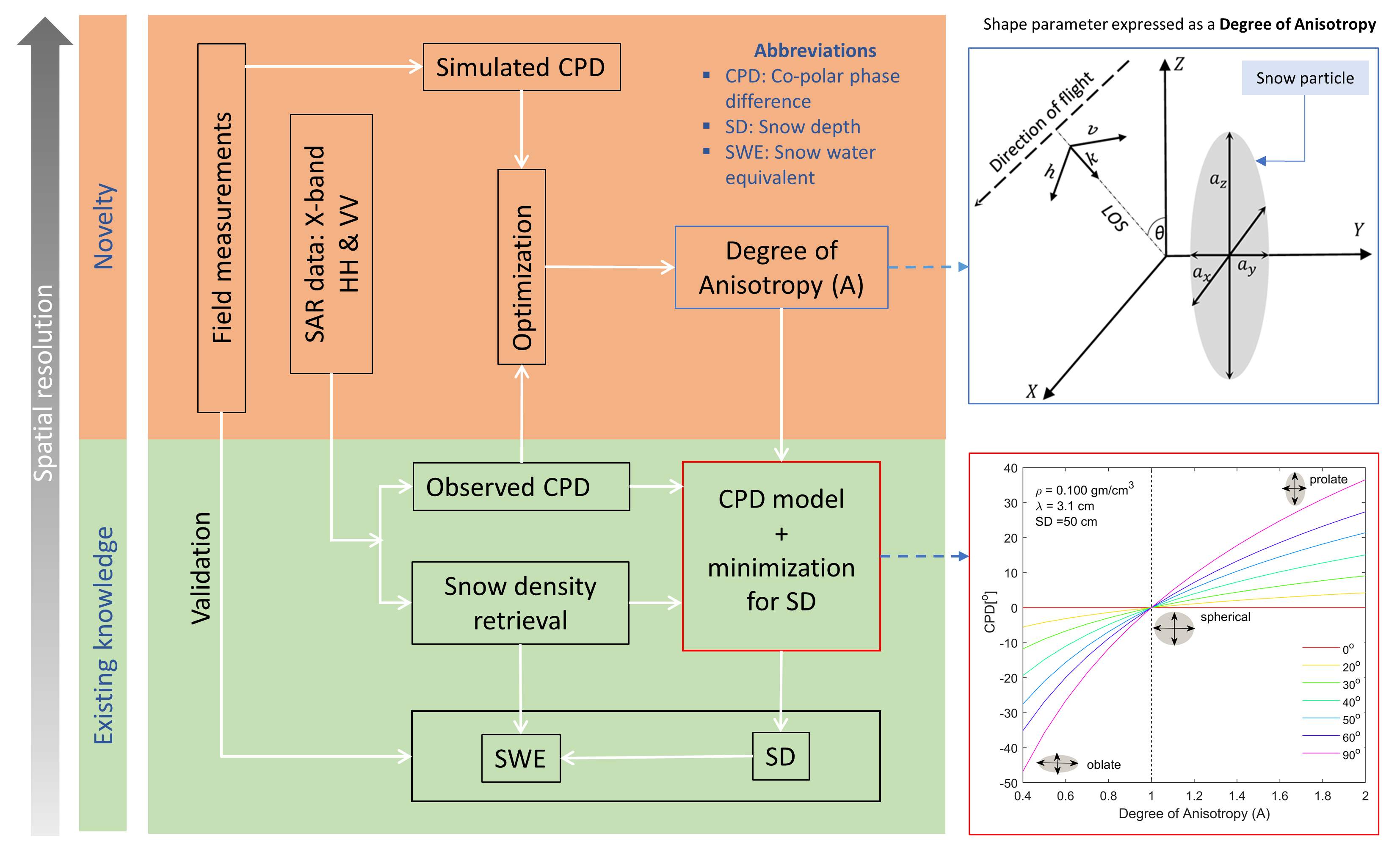
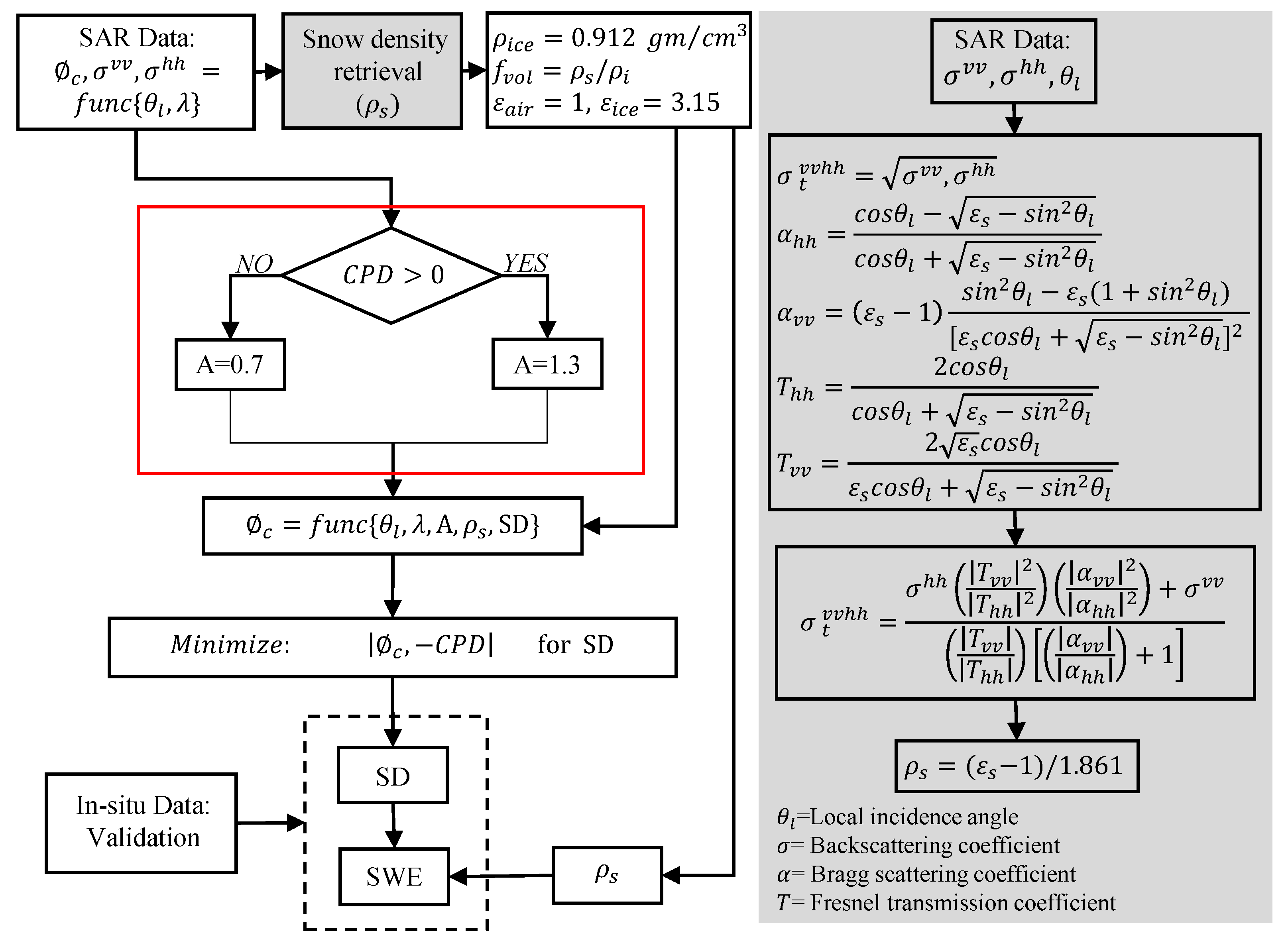
2.3. Particle Anisotropy and Snow Depth

Snow is a randomly structured medium formed by ice grains, air, and water. Settling processes and metamorphism lead to different stages of the snowpack. Fresh snow is an isotropic medium with horizontally aligned structure, and over time, due to its recrystallization and vertical temperature gradient, the snowpack transforms into a vertically aligned anisotropic medium [8]. The particle anisotropy is responsible for the thermal and dielectric properties of the snowpack [15] and is defined by the Degree of Anisotropy (A). Figure 2 shows the 3-D framework defining the structural anisotropy of the snow particle. The dielectric anisotropy results in the effective permittivity of the medium being different along the three orthogonal directions. Three dipoles of length $a_y$, $a_x$, and $a_z$ represent the spheroidal particle in the Cartesian coordinates. The shape of a spheroid is controlled by A, which is equal to the axial ratio ($a_z$/$a_x,a_x=a_y$). For oblates, the axial ratio is less than one ($a_x=a_y>a_z$). Conversely, a ratio greater than one ($a_x=a_y<a_z$) represents prolate particles. The spherical particle has a vertical-to-horizontal ratio equal to one ($a_x=a_y=a_z$). The effective permittivity of the mixture formed by aligned spheroidal ice particles with permittivity ${ϵ}_{ice}$ in the air medium of permittivity ${ϵ}_{air}$ is a function of the depolarization factor (N), which makes the effective permittivity (${ϵ}_{eff}$) direction-dependent, i.e., anisotropic.

The mathematical expression for the depolarization factor is given by [16]. The depolarization factor in the direction $a_i(i\in x,y,z)$ is

$$N_i=\frac{a_x{a}_y{a}_z}{2}{\int }_0^{\infty }\frac{ds}{(s+a_i^2)\sqrt{(s+a_x^2)(s+a_y^2)(s+a_z^2)}}$$

(2)

where s is the integration variable (expressed in area, i.e., distance square), and $ds$ represents the differential area. In this paper, we have used special cases of Equation (2) for selecting the depolarization factors which is summarized in

Table 2. Special cases of the depolarization factors $N_i(i\in x,y,z)$ for prolate and oblate particle shapes, particle shape is controlled by degree of anisotropy (A) given by axial ratio ($a_z/a_x$).

Prolate $({\mathit{a}}_{\mathit{z}}>{\mathit{a}}_{\mathit{x}}={\mathit{a}}_{\mathit{y}})$	Oblate $({\mathit{a}}_{\mathit{z}}<{\mathit{a}}_{\mathit{x}}={\mathit{a}}_{\mathit{y}})$
$N_z=\frac{1-e^2}{2e^3}\left(ln\frac{1+e}{1-e}-2e\right)$	$N_z=\frac{1+e^2}{e^3}(e-{tan}^{-1}e)$
$N_x=N_y=0.5(1-N_z)$	$N_x=N_y=0.5(1-N_z)$
$e=\sqrt{1-{\left(\frac{a_z}{a_x}\right)}^2}$	$e=\sqrt{{\left(\frac{a_x}{a_z}\right)}^2-1}$

. Using the dielectric mixing formula and Maxwell Garnett (MG) theory [16], ${ϵ}_{eff}$ of the mixture formed by air (host) and ice particles (inclusion) in Cartesian coordinates is given by

$${ϵ}_{eff}={ϵ}_{air}+\mu {ϵ}_{air}\frac{{ϵ}_{ice}-{ϵ}_{air}}{{ϵ}_{air}+(1-\mu )N_i({ϵ}_{ice}-{ϵ}_{air})}$$

(3)

where $i\in x,y,z;\mu ={\rho }_{snow}/{\rho }_{ice};$ and $\rho$ is expressed in gm/cm³. Equation (3) is transformed into radar coordinate $(h,v,k)$ by utilizing the incidence angle ($\theta$). The refractive indices for H and V polarization are given by $n_H$ and $n_V$, respectively.

$$n_H=\sqrt{{ϵ}_{eff,H}}=\sqrt{{ϵ}_{eff,x}}$$

(4)

$$n_V=\sqrt{{ϵ}_{eff,V}}=\sqrt{{ϵ}_{eff,y}{cos}^2\theta +{ϵ}_{eff,z}{sin}^2\theta }$$

(5)

The simulated co-polar phase difference (${\varphi }_c$) is a function of specific birefringence ($\Delta n=n_H-n_V$), wavelength ($\lambda$), and snow thickness (l) given by [8],

$${\varphi }_c=\frac{2\pi l}{\lambda }\Delta n$$

(6)

The simulation of Equation (6) at X-band for multiple incidence angles is shown in Figure 3.

The simulation results suggest that ${\varphi }_c$ increases with an increase in the incidence angle. For an axial ratio equal to 1 (spherical shape), the ${\varphi }_c$ is zero due to there being no delay between the HH and VV signals. As the axial ratio deviates from unity, the ${\varphi }_c$ tends to increase in either positive (prolate shape) or negative (oblate shape) direction based on the orientation of the snow particle. The value of A has been determined by optimizing the difference between CPD (Equation (1)) and ${\varphi }_c$ (Equation (6)). The field measured snow depth, density, and the local incidence angle (${\theta }_l$: derived from SRTM digital elevation model (DEM)) were used in the optimization procedure. The value of A has been determined separately for the prolate and oblate shapes. The optimization of the oblate shape results A in the range 0.68–0.71, while A ranges between 1.28–1.31 for prolate shape. The range of A was decided by providing different thresholds (1°–5°) on the difference between ${\varphi }_c$ and CPD. In this paper, we selected 0.7 and 1.3 as a threshold value for A, and used in the proposed algorithm given in Figure 4. The snow density retrieval algorithm is highlighted in Figure 4 in gray. It uses the backscattering coefficients, Fresnel transmission coefficients, and Bragg scattering coefficients at HH and VV polarization, along with ${\theta }_l$ as input parameters.

The CPD, ${\rho }_s$, A, and constant parameters related to the ice and air were provided as an input to the SD and SWE retrieval algorithm. Over the surfaces with slope ≃ 0, the CPD shows the variation with SD but does not change the sign. However, across the terrain with highly variable relief, the sign of CPD changes over short spatial scales. This scenario was observed near the Dhundi observatory, the spatial change in the CPD can be seen in Figure 5.

3. Results

The ${\rho }_s$ was retrieved from dual-pol (HH-VV) SAR data using the algorithm given in Figure 4, which was provided as an input to the SD estimation algorithm. The SD inversion was carried out iteratively by minimizing the difference between CPD and ${\varphi }_c$ for the range of SD values. The output of the minimization (inverted SD) was multiplied with ${\rho }_s$ to retrieve the SWE values. The final SD and SWE output were averaged with a 9 × 9 square window, resulting in SD and SWE maps at 90 m spatial resolution. Figure 5 shows the SD and SWE retrieved using the proposed algorithm, and the normalized-difference snow index (NDSI) calculated using the Landat-8 data over the Dhundi observatory for January 2016, generated using the Climate Engine toolbox [17]. The observatory was covered with snow during the field campaign. However, the NDSI shown in Figure 5 is higher on 8 and 30 January 2016 due to fresh snowfall (on 6, 7, and 29 January 2016).

Heavy snowfall of around 35 cm was recorded between 6 and 8 January 2016. The snowpack was dry (old snow at the bottom) with no depth hoar and crust. The average retrieved SD and SWE on 8 January 2016 are 50.23 cm and 45.89 mm, respectively. The retrieved values of the SD and SWE are expected to be less than the in situ SD and SWE due to the limited penetration of electromagnetic (EM) signals into the snowpack. However, the difference between the retrieved and measured SD is less (∼5 cm) as compared to SWE (almost half of the measured value) due to the low retrieved values of ${\rho }_s$ for dry snow condition on 8 January 2016.

No significant snowfall was recorded between 8 and 25 January 2016. The snowpack on 19 January 2019 was dry and compact with recrystallized snow formed due to melting, temporal change, and diurnal variations. The average measured ${\rho }_s$ and w on 19 January 2016 were 0.192 gm/cm${}^3$ and 1.42%VOL, respectively, at the time of the satellite acquisition (6:00 AM IST). The average retrieved SD and SWE were 35.16 cm and 64.73 mm, respectively.

Two minor snowfall events of 8 cm and 6 cm were recorded on 26 and 27 January 2016, respectively. The previously recrystallized snowpack was subsequently transformed into layers with distinct boundaries. Heavy snowfall of 30 cm was recorded on 30 January 2016. The ground measurements showed high values of w at the bottom layers (22 cm from the ground) with hard crust layers in-between. The minor snowfall thermally insulated the bottom layer, thus preserving it from further melting. Due to the distinct boundary between fresh and recrystallized snowpack (with high w), the estimated SD and SWE showed comparatively more difference than earlier estimates (8 and 19 January 2016). The estimated SD and SWE on 30 January 2016 are 34.17 cm and 55.29 mm, respectively.

Figure 6a shows the validation of SD and SWE estimated using the proposed algorithm. The SD estimation for 8 and 19 January 2016 correlates well with the field measured values, and the underestimation in SD and SWE is seen on 30 January 2016 (due to less penetration or high wetness). In Figure 6b, the SWE has been calculated by multiplying the field based density and retrieved SD. It is noticed that the SWE retrieval accuracy is better when corrected for lower density values using field measurements.

Table 3. Validation of snow depth (SD), and snow water equivalent (SWE).

Acquisition Date	Measured		Retrieved
	SD (cm)	SWE (mm)	SD (cm)	SWE (mm)
2016/01/08	41.75	47.42	47.04	63.20
	52.11	86.69	48.31	46.21
	60.42	99.89	54.33	27.19
	64.66	104.4	51.23	46.98
Average	54.73	84.61	50.23	45.89
2016/01/19	34.50	61.39	29.30	56.58
	39.50	71.05	32.55	77.91
	42.00	83.36	34.62	72.58
	44.16	84.88	43.55	59.79
	49.80	98.16	35.77	56.80
Average	41.99	79.77	35.16	64.73
2016/01/30	52.00	58.46	40.93	73.29
	59.00	112.9	20.09	43.27
	63.28	102.7	30.19	43.96
	73.85	130.1	45.46	60.62
Average	62.03	101.0	34.17	55.29

shows the validation chart for SD and SWE. Three statistical indices are used for the evaluation of the algorithm: root mean square error (RMSE), mean absolute difference (MAD), and percentage error (PR) as shown in

Table 4. Statistical analysis of the retrieved snow depth (SD) and snow water equivalent (SWE), using root mean square error (RMSE) and mean absolute difference (MAE).

Data Sets	MAE		RMSE		Percentage Error (PE)
	SD (cm)	SWE (mm)	SD (cm)	SWE (mm)	SD (%)	SWE(%)
2016/01/08	6.62	46.38	7.48	49.65	8.22	45.76
2016/01/19	6.83	17.32	7.88	21.41	16.26	18.85
2016/01/30	27.86	51.70	29.73	57.78	44.19	45.25

. It is observed that the difference between measured and retrieved SWE on 19 January 2016 is the smallest as compared to other dates, and the SD inversion results show similar accuracy on 8 and 19 January 2016. The underestimation of SWE on 8 January 2016 is due to the low retrieved value of ${\rho }_s$. Contrarily, the underestimation in SWE on 30 January 2016 is due to the limited penetration caused by wet layers (evident in the retrieved SD). The RMSE and MAD values of SD and SWE for 30 January 2016 are much higher compared to 8 and 19 January 2016, due to the formation of the layering structure with high wetness in the bottom layers. On the other hand, a snowpack with no layering and recrystallized dry snow (on 8 and 19 January 2016) resulted in a better estimation and less RMSE and MAE.

4. Summary and Discussion

In this paper, dual-polarization SAR data at X-band was used for the retrieval of the SD and SWE. The algorithm used SAR-derived CPD, particle anisotropy, snow density, and the local incidence angle for the inversion of SD. The CPD model proposed by [8] was used to optimize the particle anisotropy for the prolate and oblate shapes. A spatially variable ${\rho }_s$ calculated using an algorithm (summarized in Figure 4) given by [11] was used for the SWE retrieval. In the process, a spatial resolution of 90 m was achieved for SD and SWE. The SD and SWE inversion accuracy was tested with three SAR acquisitions covering different characteristics (in terms of layering and wetness) of the snowpack, i.e., fresh snow on top of the old snow (8 January 2016), recrystallized snow (19 January 2016), and layered snowpack with high wetness (30 January 2016)). We have noticed that the algorithm performance is satisfactory for recrystallized snow with no hard crust.

The SD inversion shows good accuracy on 8 and 19 January 2016 (average MAE = 6.5 cm, RMSE = 7.5 cm, and PE = 12.24%). Likewise, SWE retrieval on 19 January resulted in MAE = 17.32 mm, RMSE = 21.41 mm, and PE = 18.85%. However, the SWE retrieval shows underestimation on 8 January 2016 (due to low retrieved ${\rho }_s$ values) and 30 January 2016 (due to low penetration), respectively. Hence, it is found that the inversion algorithm appears to have acceptable accuracy for SD and SWE in the case of the recrystallized snowpack. Also, good accuracy of SD inversion is noticed for the snowpack formed with fresh and old snow with low wetness. The ground-based experiments to measure CPD at high temporal resolution can add more information on the behavior of CPD. In the future, we will focus on improving the retrieval of SD and SWE for complex snowpack.

References

1. Tsai, Y.L.S.; Dietz, A.; Oppelt, N.; Kuenzer, C. Remote Sensing of Snow Cover Using Spaceborne SAR: A Review. Remote Sens. 2019, 11, 1456. [Google Scholar] [CrossRef] [Green Version]
2. Bolch, T.; Shea, J.M.; Liu, S.; Azam, F.M.; Gao, Y.; Gruber, S.; Immerzeel, W.W.; Kulkarni, A.; Li, H.; Tahir, A.A.; et al. Status and Change of the Cryosphere in the Extended Hindu Kush Himalaya Region. In The Hindu Kush Himalaya Assessment; Wester, P., Mishra, A., Mukherji, A., Shrestha, A.B., Eds.; Springer International Publishing: Cham, Switzerland, 2019; pp. 209–255. [Google Scholar] [CrossRef] [Green Version]
3. Mityók, Z.K.; Bolton, D.K.; Coops, N.C.; Berman, E.E.; Senger, S. Snow cover mapped daily at 30 meters resolution using a fusion of multi-temporal MODIS NDSI data and Landsat surface reflectance. Can. J. Remote Sens. 2018, 44, 413–434. [Google Scholar] [CrossRef]
4. Saberi, N.; Kelly, R.; Flemming, M.; Li, Q. Review of snow water equivalent retrieval methods using spaceborne passive microwave radiometry. Int. J. Remote Sens. 2020, 41, 996–1018. [Google Scholar] [CrossRef]
5. Deems, J.S.; Painter, T.H.; Finnegan, D.C. Lidar measurement of snow depth: A review. J. Glaciol. 2013, 59, 467–479. [Google Scholar] [CrossRef] [Green Version]
6. Rott, H.; Yueh, S.H.; Cline, D.W.; Duguay, C.; Essery, R.; Haas, C.; Hélière, F.; Kern, M.; Macelloni, G.; Malnes, E.; et al. Cold Regions Hydrology High-Resolution Observatory for Snow and Cold Land Processes. Proc. IEEE 2010, 98, 752–765. [Google Scholar] [CrossRef] [Green Version]
7. Kurtz, N.T.; Farrell, S.L.; Studinger, M.; Galin, N.; Harbeck, J.P.; Lindsay, R.; Onana, V.D.; Panzer, B.; Sonntag, J.G. Sea ice thickness, freeboard, and snow depth products from Operation IceBridge airborne data. Cryosphere 2013, 7, 1035–1056. [Google Scholar] [CrossRef] [Green Version]
8. Leinss, S.; Parrella, G.; Hajnsek, I. Snow Height Determination by Polarimetric Phase Differences in X-Band SAR Data. IEEE J. Sel. Top. Appl. Earth Obs. Remote. Sens. 2014, 7, 3794–3810. [Google Scholar] [CrossRef] [Green Version]
9. Leinss, S.; Löwe, H.; Proksch, M.; Lemmetyinen, J.; Wiesmann, A.; Hajnsek, I. Anisotropy of seasonal snow measured by polarimetric phase differences in radar time series. Cryosphere 2016, 10, 1771–1797. [Google Scholar] [CrossRef] [Green Version]
10. Majumdar, S.; Thakur, P.; Chang, L.; Kumar, S. X-band polarimetric sar copolar phase difference for fresh snow depth estimation in the Northwestern Himalayan watershed. In Proceedings of the 2019 IEEE International Geoscience and Remote Sensing Symposium, IGARSS 2019, Yokohama, Japan, 28 July–2 August 2019; pp. 4102–4105. [Google Scholar] [CrossRef]
11. Singh, G.; Venkataraman, G. Snow density estimation using Polarimitric ASAR data. In Proceedings of the 2009 IEEE International Geoscience and Remote Sensing Symposium, Cape Town, South Africa, 12–17 July 2009. [Google Scholar]
12. Cuerda Munoz, J.M.; Rodriguez, M.G.; Gonzalez Bonilla, M.J.; Vazquez, N.C.; Revenga, P.C.; Martinez, N.G.; Pescador, A.L. INTA Commissioning Phase Plan for PAZ Mission. In Proceedings of the 12th European Conference on Synthetic Aperture Radar, Aachen, Germany, 4–7 June 2018; pp. 1–4. [Google Scholar]
13. Snow Fork. Available online: https://toikkaoy.com/Snowfork.htm (accessed on 21 November 2019).
14. Lee, J.S.; Pottier, E. Polarimetric Radar Imaging: From Basics to Applications; Number 142 in Optical Science and Engineering; CRC Press/Taylor & Francis: Boca Raton, FL, USA, 2009. [Google Scholar]
15. Löwe, H.; Riche, F.; Schneebeli, M. A general treatment of snow microstructure exemplified by an improved relation for thermal conductivity. Cryosphere 2013, 7, 1473–1480. [Google Scholar] [CrossRef] [Green Version]
16. Sihvola, A. Mixing Rules with Complex Dielectric Coefficients. Subsurf. Sens. Technol. Appl. 2000, 1, 393–415. [Google Scholar] [CrossRef]
17. Climate Engine. Available online: https://climateengine.org/ (accessed on 22 November 2019).
Figure 1. (a) SRTM digital elevation model (DEM), and (b) slope over study area.
Remotesensing 12 01183 g001
Figure 2. The spheroidal represents a vertically aligned prolate ice particle in the Cartesian coordinate system. The direction of wave propagation is given by vector k, the h and v vectors represent the horizontal and the vertically polarized wave, and θ is incidence angle. The degree of anisotropy is given by axial ratio ( a z / a x ). The spheroidal has width a x or a y ( a x = a y ), and the length a z (adapted from [8]).
Remotesensing 12 01183 g002
Figure 3. The simulated co-polar phase difference ( ϕ c ) as a function of degree of anisotropy (A), snow depth (SD), ρ s , λ , and incidence angle.
Remotesensing 12 01183 g003
Figure 4. The snow depth (SD) and snow water equivalent (SWE) inversion using dual polarization (HH-VV) synthetic aperture radar (SAR) data. The snow density ( ρ s ) retrieval algorithm is highlighted in gray.
Remotesensing 12 01183 g004
Figure 5. Co-polar phase difference (CPD (ac)), snow depth (SD (df)), snow water equivalent (SWE (gi)), and normalized difference snow index (NDSI (jl)) over Dhundi observatory retrieved using the proposed algorithm for: 8 January 2016 (first column), 19 January 2016 (second column), and 30 January 2016 (third column). Forest mask was generated using ALOS data, NDSI was retrieved using Landsat -8 data, and layover shadow mask was generated using 12 meter ALOS digital elevation model. The location of Dhundi observatory is highlighted by blue (first row), white (second and third row), and yellow (fourth row) polygons. The magenta dots represents the location of validation points.
Remotesensing 12 01183 g005
Figure 6. (a) Validation plot for snow depth (SD) and snow water equivalent (SWE) retrieved using the proposed algorithm. (b) Snow water equivalent (SWE) calculated by multiplying the field based density and retrieved snow depth (SD).
Remotesensing 12 01183 g006