An Improved Res-UNet Model for Tree Species Classification Using Airborne High-Resolution Images

Abstract

Tree species classification is important for the management and sustainable development of forest resources. Traditional object-oriented tree species classification methods, such as support vector machines, require manual feature selection and generally low accuracy, whereas deep learning technology can automatically extract image features to achieve end-to-end classification. Therefore, a tree classification method based on deep learning is proposed in this study. This method combines the semantic segmentation network U-Net and the feature extraction network ResNet into an improved Res-UNet network, where the convolutional layer of the U-Net network is represented by the residual unit of ResNet, and linear interpolation is used instead of deconvolution in each upsampling layer. At the output of the network, conditional random fields are used for post-processing. This network model is used to perform classification experiments on airborne orthophotos of Nanning Gaofeng Forest Farm in Guangxi, China. The results are then compared with those of U-Net and ResNet networks. The proposed method exhibits higher classification accuracy with an overall classification accuracy of 87%. Thus, the proposed model can effectively implement forest tree species classification and provide new opportunities for tree species classification in southern China.

1. Introduction

Tree species classification is highly significant for sustainable forest management and ecological environmental protection [1]. High-spatial-resolution remote sensing images are preferred for detailed tree classification because of their better spatial characteristics.

In recent years, significant advances have been made in high-scoring image classification methods, which are typically characterized into pixel-based classification [2,3,4] or object-oriented classification [5,6,7,8]. Pixel-based classification methods use pixels as the unit of classification; they mainly consider the band spectral intensity information of the pixel and ignore the spatial structure relationship and contextual semantic information [9]. For high-resolution remote sensing images with fewer bands, pixel-based methods will lead to substantial redundancy in the spatial data, resulting in “salt and pepper” effects. Many scholars combined manual feature extraction with traditional object-oriented methods for tree species classification. Immitzer et al. [10] performed a Random Forest classification (object-based and pixel-based) using spectra of manually delineated sunlit regions of tree crowns and the overall accuracy for classifying 10 tree species was around 82%. Li et al. [11] explored the potential of bitemporal WorldView-2 and WorldView-3 images for identifying five dominant urban tree species with the object-based Support Vector Machine and Random Forest methods. The study showed that tree species classification accuracy is higher in bitemporal images. Ke et al. [9] used three segmentation schemes to evaluate the synergistic use of high spatial resolution multispectral imagery and low-posting-density LiDAR data for forest species classification using an object-based approach and synergistic use improved the forest classification. However, these methods require manual feature selection, which is subjective and therefore complicates the extraction of high-quality features [12,13,14]. With the development of deep learning [15], increasing numbers of researchers are using neural networks to automatically extract features, thereby eliminating the need for manual feature selection [16,17,18].

Since being proposed by Hinton in 2006 [19], deep learning theory has resulted in significant progress in scene recognition, object detection, and remote sensing image classification [20,21,22,23,24,25]. The most representative architecture is the convolutional neural network (CNN), which is a multilayer neural network whose design is derived from the concept of subregions and the hierarchical analysis revealed by study of the mammalian visual cortex [26]. Deep layers such as textures, boundaries, and topological structures can be obtained from feature maps, resulting in high classification scores in the classification tasks of ImageNet and PASCAL VOC (pattern analysis, statistical modeling, and computational learning visual object classes) datasets [27]. He et al. [28] proposed a method of combining saliency and multilayer CNN to classify two high-scoring image scene datasets of UC Merced 21 and Wuhan 7. Zhang et al. [29] stacked multiple fully connected layers of CNN together to extract multiscale convolutional features and perform aircraft target detection in high-scoring images. Furthermore, Khan et al. [30] solved the problem of multilabel scene classification for high-scoring images through an improved CNN network. In the field of tree species classification, it became common to use improved CNN for tree species classification. Sun et al. [31] modified three different deep learning methods (i.e., AlexNet, VGG16, and ResNet50) to classify the tree species, as they can make good use of the spatial context information and VGG16 had the best performance, with an overall accuracy of 73.25% for 18 tree species. Hartling et al. [32] used Dense Convolutional Network (DenseNet) for tree species classification and examined its ability to classify dominant tree species within a highly complex urban environment using a data fusion approach with high spatial resolution multispectral imagery and LiDAR datasets.

Typically, a CNN network will connect several fully connected layers after the convolution layer and map the feature map generated by the convolution layer into a fixed-length feature vector [33]. The general CNN structure is suitable for image-level classification and regression tasks because it desires the probability of classification of the input image at the end. However, the desired output of remote sensing image tree classification is a classification map of the same size as the input image. To solve this problem, Long et al. [34] proposed the fully convolutional network (FCN) in 2015 and explained its application to semantic segmentation. Ronneberger et al. [35] improved the FCN and proposed the U-Net network. Many subsequent classification studies are based on the idea of the FCN network. Fang et al. [36] applied the FCN to the classification of high-resolution remote sensing images; their results showed that the FCN can better obtain the essential features of ground features in images. Moreover, the mean drift segmentation algorithm can be used to optimize the edge of the obtained probability map results and improve the classification accuracy. Fu et al. [37] proposed an accurate classification approach for high-resolution remote sensing imagery based on the improved FCN model. The average precision, recall, and Kappa coefficient are 0.81, 0.78, and 0.83, respectively. Flood et al. [38] manually labeled 3-band Earth-i imagery for the presence of trees or large shrubs and used the U-net neural network architecture to map the presence or absence of trees and large shrubs across the Australian state of Queensland.

However, the FCN does not consider the spatial relationship between pixels when categorizing tree species in remote sensing images. Moreover, it lacks spatial consistency and cannot extract more useful spatial and spectral features [34]. The obtained tree species results are not sufficiently accurate and the spatial details of the images are relatively low resolution; therefore, the accuracy of the classification task is unsatisfactory for complex feature information. The U-Net network can combine the underlying spatial feature obtained by downsampling with the input of upsampling through skip connections to improve its ability to obtain tree edge information. However, gradient degradation commonly occurs during the process of network deepening. The ResNet network has a unique residual unit, which can avoid gradient degradation in the process of network deepening [39]. Introducing it into U-Net network has become a current research hotspot. Some scholars have carried out related research in the fields of single target extraction and urban land classification. Chu et al. [40] proposed a method based on U-Net that used ResNet replaced contraction part for sea-land segmentation. Xu et al. [41] designed an image segmentation neural network based on deep residual networks and used a guided filter to more effectively extract buildings in remote sensing imagery. Zhang et al. [42] proposed novel multiscale deep learning models, namely ASPP-UNet and ResASPP-UNet for urban land cover classification based on very high-resolution satellite imagery and ResASPP-UNet produced the highest classification accuracy.

However, previous studies mainly performed simple binary classification by combining U-Net and ResNet, and the network structure was relatively simple. Other studies mainly addressed urban land use classification problems and therefore the ability to classify tree species in complex forest type is not clear. The problem of small differences in spectral characteristics between tree species brought challenges to tree species classification. Therefore, the main objectives of this study include the following: to combine U-Net and ResNet and propose a Res-UNet network suitable for tree species classification. The convolutional layer of U-Net is replaced with the basic unit of ResNet, which is used to extract multiscale spatial features and simultaneously solve the gradient degradation problem of deep networks for an increasing number of network layers. At the output of the network, post-processing with the conditional random fields (CRF) is proposed to optimize the tree species segmentation graph; to evaluate the ability of airborne CCD (charge coupled devices) images to identify complex forest tree species in the south using the Res-UNet network; and to analyze the parameters that affect the classification ability of the model.

2. Materials and Methods

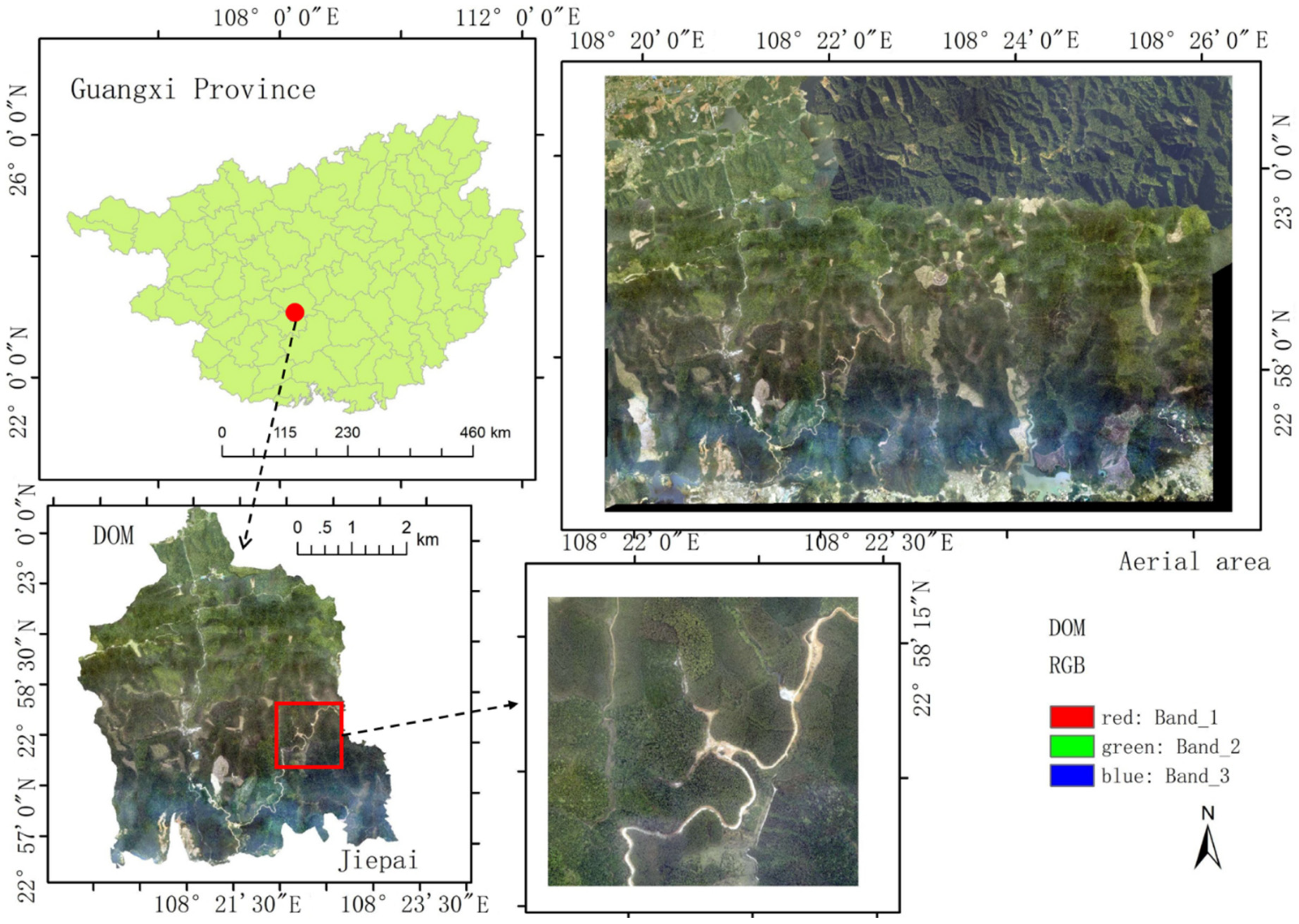
2.1. Study Area

The study area is located in the Jiepai Forest Farm of the Guangxi Gaofeng State Owned Forest Farm in Nanning, Guangxi Province, southern China. As shown in Figure 1, it is located at 108°31′ east longitude and 22°58′ north latitude. The average annual temperature is approximately 21 ℃, the average annual rainfall is 1304.2 mm, and the red soil layer is deep, which is suitable for the growth of tropical and subtropical tree species [43]. The forest cover in the study area is dominated by artificial forests, predominantly eucalyptus (Eucalyptus robusta Smith), Illicium verum (Illicium verum Hook.f.), wetland pine (Pinus elliottii Engelm.), Masson pine (Pinus massoniana Lamb.), Chinese fir (Cunninghamia lanceolata (Lamb.) Hook.), and other broad-leaved tree types. Among them, eucalyptus (Eucalyptus robusta Smith) and Chinese fir (Cunninghamia lanceolata (Lamb.) Hook.) are planted over large areas, which has certain advantages for classification. Some broad-leaved tree species have a small planting area so are classified as other broad-leaved trees. Some roads also exist in the study area. The classification system is shown in

Table 1. Classification system of the study area (Figure 1 (bottom right)).

Type	Common Name	Note
Nonforest land	Roads	Nonforest land mainly includes roads
Forest land	Other forest land	Mainly includes some auxiliary production land
	Cunninghamia lanceolata	Pure Chinese fir forests
	Eucalyptus robusta	Large area eucalyptus, there are many logging areas in the forest
	Illicium verum	Pure Illicium verum forests
	Pinus massoniana	Pure Pinus massoniana forests
	Pinus elliottii	A small amount of pure wetland pine forest land
	Mytilaria laosensis	Mytilaria laosensis and Chinese fir mixed forest
	Other broad-leaved	Small amount of unknown broadleaf

.

2.2. Acquisition and Preprocessing of Remote Sensing Image Data

The aerial flights took place on January 13, 2018 and January 30, 2018. The aerial photography area was 108°7′ to 108°38′ east longitude, 22°49′ to 23°5 ′ north latitude, measuring approximately 125 km². The specific area is shown in Figure 1. The actual flight altitude was approximately 1000 m, and the weather on the day of data acquisition was clear and cloudless. The onboard LiCHy (LiDAR, CCD, and Hyperspectral) system of the Chinese Academy of Forestry is equipped with an aerial digital camera to acquire CCD images [44]. It is also equipped with a LiDAR scanner and a hyperspectral sensor for LiDAR Data, hyperspectral data, inertial measurement unit (IMU), and GPS data. The aviation digital camera has 60 million pixels, a lens focal length of 50 mm, and an image spatial resolution of 0.2 m, including three bands of red, green, and blue.

2.3. Ground Survey Data and Other Auxiliary Data

The ground data survey was conducted at Gaofeng Forest Farm from January 16, 2018 to February 5, 2018. First, the GF-2 data were visually interpreted to determine the location of the classification area. Then field survey was conducted in the classification area to understand the distribution and characteristics of tree species. In addition, a vector map of the entire forest farm provided by the Guangxi Academy of Forest Sciences was used to assist in making labels for training samples.

2.4. Datasets Production

The datasets used in this study were cropped from the entire image of entire aerial area (as shown in Figure 1 (top right)). The training data comprised 1000 images with a pixel size of 1024 × 1024 including all categories in the classification system. The test data size was 5334 × 4951 pixel images and training data and test data are independent of each other. Based on forest farm vector data, visual interpretation, and a field survey, the tree species categories were marked as labels. In order to meet the required number of samples during the training process, data enhancement operations such as translation and rotation were performed on the training data to form a total of 2000 images that were sent to the neural network as a training set. To enhance the robustness of the network, the training sets were divided into training data (80%) and validation data (20%) using the stratified sampling method. The number of training samples and validation samples in each category is shown in

Table 2. Number of training and validation samples for each tree species category after data augmentation.

Type	Training Samples	Validation Sample
Eucalyptus	288	72
Illicium verum	260	65
Roads	120	30
Pinus massoniana	168	42
Mytilaria laosensis	111	28
Other broad-leaved	76	19
Other forest land	200	50
Chinese fir	224	56
Pinus elliottii	153	38
Total	1600	400

. In addition, this study used 40%, 60%, 80%, and 100% of the training sets for training in order to explore the most suitable number of training samples.

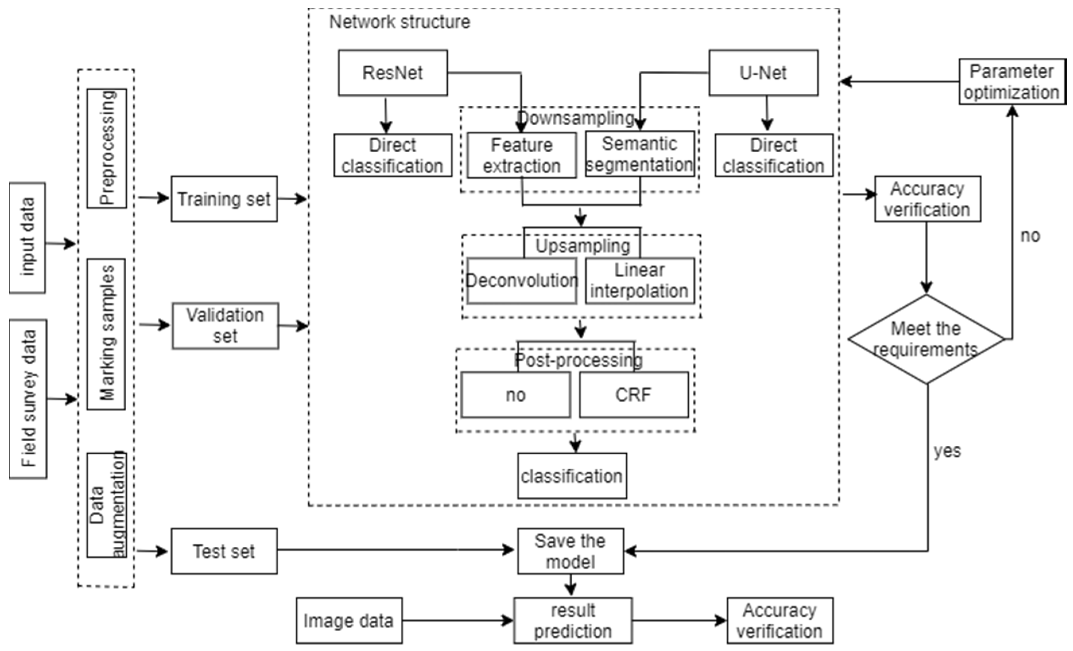
2.5. Workflow Description

In this study, an improved U-Net network was used to classify high-resolution images of tree species. The convolutional layer of the network was represented by the residual unit of the ResNet network. The classification process was shown in Figure 2: 1024 × 1024 image blocks were cut from the entire image and the real feature categories were labeled as training samples. The training samples were used as the training set after image enhancement. The selected test sample size was 5334 × 4951, which contained nine feature types. The same method was used to label the true feature types. The image block instead of the pixel unit was sent to the network for training, and the model loss was obtained after training. The model parameters were updated by gradient back propagation until the optimal parameters were obtained. In the classification stage, the test set was sent to the trained network for prediction, and the prediction result was subjected to CRF post-processing to obtain the final classification map.

2.6. Network Structure

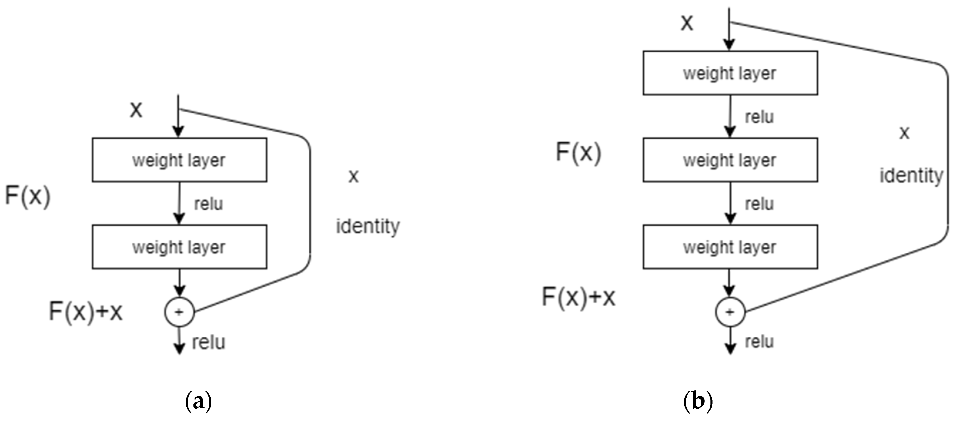
2.6.1. ResNet Network

Kaiming He et al. [39] proposed the ResNet network in 2015, which won first place in the ImageNet competition classification task. ResNet was proposed to solve the problem of deep gradient degradation. Thus, many subsequent methods have been based on either ResNet50 or ResNet101. ResNet refers to the VGG19 network on which it is based; it replaces the fully connected layer with a global average pool and uses a connection method called “shortcut connection” (see Figure 3). The feature map is composed of a residual map and an identity map and the output is y = F (x) + x. Residual learning is easier than original feature learning. When the network has reached the optimum, it continues to deepen and the residual approaches zero. At this time, the network only performs identity mapping, and its performance does not decrease with increasing depth, which avoids the degradation problem caused by network deepening. In this study, two residual units were designed for different model requirements. As shown in Figure 4, when the number of input channels and output channels was equal, the residual unit shown in Figure 4a was used to perform three 3 × 3 convolution operations on the input and output together with the original input, using a stride of one. Conversely, when the number of input channels and output channels was different, the residual unit of Figure 4b was used with a stride customized, and 3 × 3 convolution was performed on the input and output with the results after three convolution operations. The ResNet network in this study was composed of these two types of residual units. In order to achieve the tree species classification task, the residual unit 4b was used at the output end of the network instead of the fully connected layer. A two-dimensional feature map was output, and softmax was used for pixel-by-pixel class prediction.

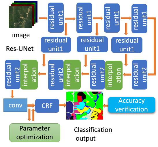
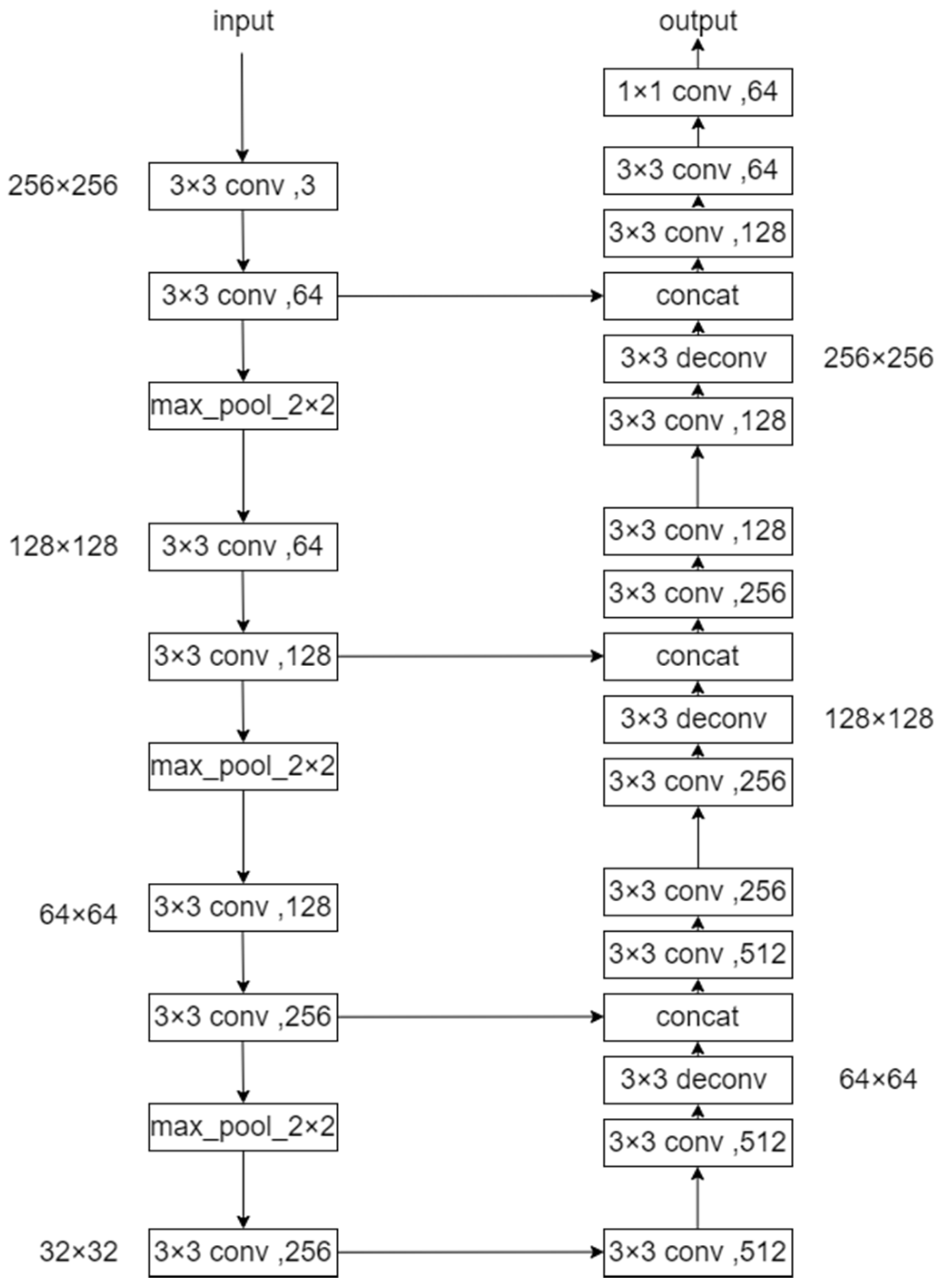
2.6.2. ResNet-Unet Network

Previously, when CNN was used for classification tasks, the input could only take the form of images and the output was the corresponding labels; however, many users wish to obtain the classification results for each pixel in visual tasks. Ronneberge et al. [35] proposed the U-Net network in 2015, whose network structure is shown in Figure 5. In the structure, “3 × 3 conv, n” represents the convolution layer with a convolution kernel of 3 × 3 and number of input channels is n, “max_pool_2 × 2” represents the maximum pooling layer with a step size of two, “3 × 3 deconv” represents the convolution kernel with a 3 × 3 transposed convolution layer, “concat” refers to splicing two tensors, and “m × m” such as “256 × 256” means m-m size of feature map. It was mainly used for medical image analysis, before gradually being used in image classification tasks. U-Net is also a variant of the CNN that has been improved using FCN. U-Net is composed of two main parts: the contraction path and the expansion path. The contraction path is used to capture the semantic information of the image, whereas the symmetrical expansion path is used to accurately locate the semantic information. The fully connected layer is not used in the network structure. It reduces the number of parameters that need to be trained, enabling the network to perform end-to-end output more efficiently.

Our tree classification strategy used the idea of semantic segmentation. Based on the advantages of the U-Net network, this study proposed a Res-UNet network by combining U-Net and ResNet and the following improvements were made for the classification of tree species: (1) The convolutional layer, pooling layer, and residual unit were modified. (2) A residual unit was inserted to extract the image space features before fusing the feature maps of the downsampling layer and the upsampling layer, so as to adapt to the classification of complex tree species. (3) Linear interpolation was used instead of deconvolution to reduce the model complexity to a certain extent. (4) The final output level was modified to nine to distinguish the nine tree species. (5) At the output of the network, post-processing with the CRF is proposed to optimize the tree species segmentation graph. The network structure was shown in Figure 6. It includes downsampling and upsampling. In the structure, “3 × 3 conv, n” and “m × m” such as “256 × 256” have the same meaning as U-Net, “resize_bilinear” represents bilinear interpolation, and “add” refers to connecting two matrices.

In the downsampling network structure, four residual units with a step size of two are used for feature extraction. Every time the feature map passes through a residual unit, its size is doubled and the number of convolution filters is doubled. In each residual unit, the data is normalized in batches to ensure that each forward propagation is output on the same distribution as the maximum. In this way, the distribution of the data samples referenced in the backward calculation will be the same as that in the forward calculation, ensuring a uniform distribution, leading to more meaningful adjustment of the weights and avoiding the problem of gradient explosion during network training. The activation function is rectified linear unit (relu), which enables the sparse model to better mine relevant features and fit the training data to accelerate network convergence.

When using a full CNN for high-scoring image classification, in order to achieve end-to-end classification, deconvolution is often used for upsampling operations to upsample the feature map to the size of the input image. However, deconvolution needs to learn a large number of parameters and is computationally intensive. The bilinear interpolation algorithm does not require learning parameters, reducing the amount of calculation [45]. Therefore, this study used bilinear interpolation instead of deconvolution and analyzed its impact on classification performance. So, in the upsampling network, a linear interpolation operation is used instead of deconvolution. Every time the linear interpolation is performed, the feature map is doubled until it increases to the size of the input feature map, so that the entire network can achieve end-to-end input. In the linear interpolation process, as the number of convolutions increases, the extracted features are more effective; however, the loss of feature map spatial information can easily occur. Therefore, feature maps with the same size in the upsampling layer and downsampling layer are combined to obtain a feature map with higher spatial resolution.

In this study, the downsampled feature map was first sent to a residual unit with a step size of 1 then upsampled. When the upsampling features were fused, the output of each layer of the upsampling was first subjected to a residual operation with a step size of one to ensure that it has the same size and number of channels as the corresponding upsampling layer. At the output of the network, a 1 × 1 convolution layer was used to obtain a feature map with the same number of output channels as categories. The proposed Res-UNet network enables the feature map to be restored to the input size by extracting the deep features of the image to achieve end-to-end classification.

2.7. Conditional Random Field (CRF)

The CRF is a discriminant probability model, which is an improvement on the Hidden Marko Model (HMM) and Maximum Entropy Markov Model (MEMM). CRF overcomes the limitation of HMM whereby it can only define specific types of feature functions. Instead, the CRF can define a larger number of feature functions, and the feature functions can use arbitrary weights. MEMM is only normalized locally; thus, it is easy to fall into local optimization. In the CRF model, the global probability is counted. When normalizing, the global distribution of the data is considered, the problem of label offset of the MEMM is solved, and the global optimum can be obtained.

In image segmentation, CRF treats each labeled pixel as a random variable in a Markov random field, and the entire image is a global observation. Then, the energy function labeled x can be expressed as:

$$\mathrm{E}\left(\mathrm{x}\right)={\mathsf{\Sigma }}_{\mathrm{i}}{\mathsf{\phi }}_{\mathrm{u}}\left({\mathrm{x}}_{\mathrm{i}}\right)+{\mathsf{\Sigma }}_{\mathrm{i}<\mathrm{j}}{\mathsf{\phi }}_{\mathrm{p}}\left({\mathrm{x}}_{\mathrm{i}},{\mathrm{x}}_{\mathrm{j}}\right)$$

(1)

The first item is a data item, which is the segmentation result of CNN, and it represents the probability that the xi-th pixel belongs to each category. The second term is a post-processing smoothing term, which represents the difference in gray value and spatial distance between the two pixels xi and xj. At this time, the most likely label combination can be obtained by minimizing the energy function E (x). Then, the optimal segmentation result can be obtained. Post-processing is critical to the classification results. In order to verify the impact of the classification results using CRFs for post-classification processing, a CRF operation was added to the network output.

2.8. Network Training and Prediction

During network training, the model parameters were initialized randomly and the training set was input into the model for training. The average cross-entropy loss was used to calculate the loss of the model, where the loss function is expressed as follows:

$$\mathrm{loss}=-\frac{1}{\mathrm{m}}{\displaystyle \sum }_{\mathrm{i}=1}^{\mathrm{m}}[{\mathrm{x}}_{\mathrm{i}}\log \left({\mathrm{z}}_{\mathrm{i}}\right)+(1-{\mathrm{x}}_{\mathrm{i}})\log \left(1-{\mathrm{z}}_{\mathrm{i}}\right)]$$

(2)

Here, m represents the size of the mini-batch, and x_i and z_i represent the predicted and true values of the ith sample in each batch, respectively. The loss was forwarded and the network parameters were optimized using the Adam optimizer [46]. The calculation formula of the Adam optimizer is

$${\mathsf{\theta }}_{\mathrm{t}}={\mathsf{\theta }}_{\mathrm{t}-1}-\mathsf{\alpha }\ast {\hat{\mathrm{m}}}_{\mathrm{t}}/\left(\sqrt{{\hat{\mathrm{s}}}_{\mathrm{t}}}+\mathsf{ϵ}\right)$$

(3)

where θ is the weight, α is the learning rate, t is the number of training iterations, m is the momentum vector, s is the squared cumulative vector of the gradient, and ϵ is an infinitely small number.

Finally, under the optimal model, the learning rate was set to 1e-5, the batch size was 1, and 60,000 rounds were trained until the accuracy ceases to improve. The model weights were guaranteed. During prediction, due to computer memory limitations, the model predicts the 256 × 256 area of the test image each time and uses CRF for post-processing until it traverses the entire image to obtain the classification result map. This study used Python based on the TensorFlow deep learning framework. The hardware configuration of the operating platform included IntelⓇXeon (R) CPU E5-2620 [email protected] and two nvidia GeForce GTX 1080Ti GPUs.

3. Results

3.1. Tree Species Classification Results with Different Training Samples

Table 3. Tree species classification accuracy in Res-UNet (Linear interpolation + CRF) networks with different training sample numbers.

Number of Samples	40%	60%	80%	100%
Overall Accuracy	70.41%	79.87%	84.28%	87.51%
Average Accuracy	70.09%	78.69%	82.17%	85.43%
Kappa Coefficient	0.683	0.773	0.815	0.842

shows the tree species classification accuracy in the Res-UNet (Linear interpolation + CRF) network using 40%, 60%, 80%, and 100% of the training sets. When the training sample is 40% of the training set, it shows very poor classification results, and the Kappa coefficient is only 0.683. In addition, with the increase of the training set, the classification accuracy shows an upward trend, but the increased amplitude gradually decreases. Therefore, this study used 100% of the training sets to conduct experiments with different methods.

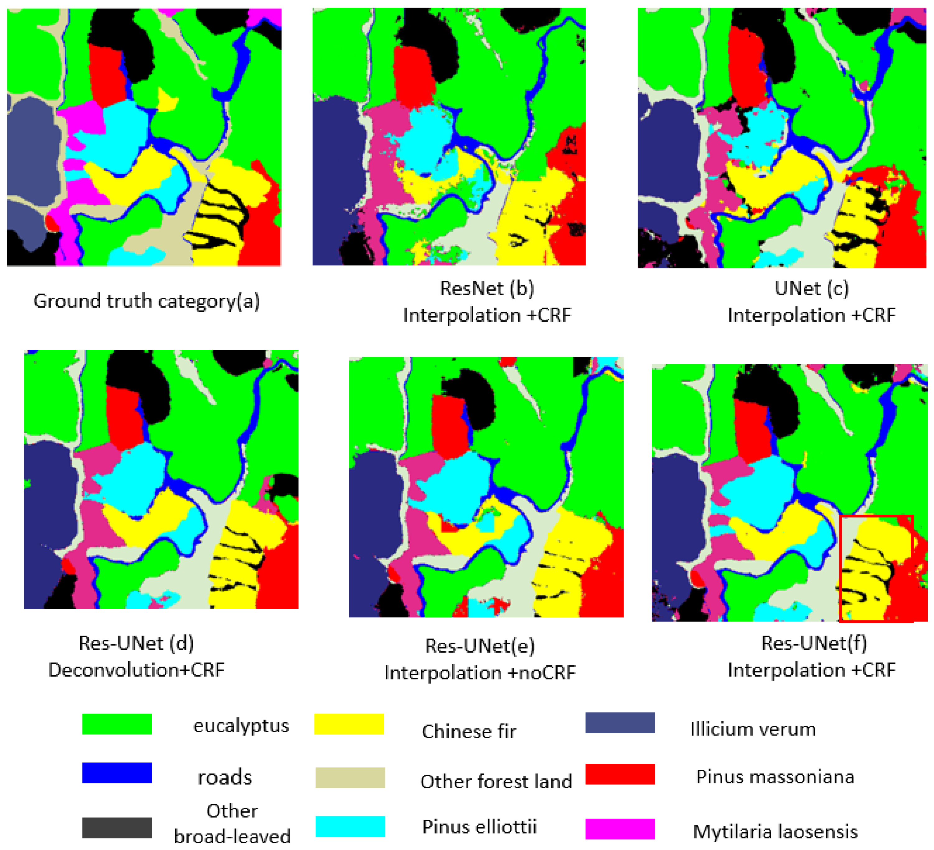
3.2. Tree Species Classification Results

Figure 7 shows the tree species classification results for various classification methods. According to the comparison and analysis of the classification results, Res-UNet has a better ability to distinguish each tree species. Eucalyptus and Illicium verum can be better classified, but the small area of Mytilaria laosensis is seriously misaligned. After post-processing with the CRF, the mixed phenomenon of Chinese fir and other broad-leaved improved.

The tree species classification results of various methods are shown in

Table 4. Classification accuracy of tree species with different classification methods.

Method	ResNet (Linear Interpolation + CRF)	UNet (Linear Interpolation + CRF)	Res-UNet (Deconvolution + CRF)	Res-UNet (Linear Interpolation + noCRF)	Res-UNet (Linear Interpolation + CRF)
Overall Accuracy (%)	68.25	75.34	81.67	84.76	87.51
Average Accuracy (%)	65.12	74.45	81.09	85.23	85.43
Kappa Coefficient × 100	65.52	73.28	80.34	83.15	84.21
Eucalyptus	71.58	80.12	87.45	88.24	88.37
Illicium verum	84.32	81.09	85.21	87.13	87.62
Roads	68.15	74.58	81.07	82.97	83.57
Pinus massoniana	69.07	76.43	86.58	85.04	87.14
Mytilaria laosensis	58.23	61.98	72.32	75.36	78.65
Other broad-leaved	49.67	54.37	51.08	66.15	70.41
Other forest land	49.82	70.13	76.42	80.73	83.14
Chinese fir	55.89	72.64	79.21	85.43	86.01
Pinus elliottii	41.45	70.51	80.34	85.03	87.15

Note: The numbers with gray background in the table indicate the highest overall classification accuracy, average classification accuracy, and Kappa coefficient among the various classification methods.

. The classification accuracy of the Illicium verum is high in various networks, indicating that various networks can effectively extract the characteristics of the Illicium verum, and the classification results are relatively stable. Except for other broad-leaved, Res-UNet improves the classification accuracy of tree species from that of ResNet and U-Net. The classification accuracy of each tree species has been improved to a different level after CRF post-processing was added; the overall classification accuracy increases by 2.7%. The classification accuracy of tree species is also improved by using bilinear interpolation instead of deconvolution, and the overall classification accuracy is improved by 5.8%. Figure 7f shows the results of post-processing and upsampling using linear interpolation, which again indicates that the proposed model achieves the best classification effect. Although the classification accuracy is lower than the results obtained using hyperspectral imagery, it shows higher classification accuracy compared to studies using three-band high-resolution image classification.

As shown in Figure 8, the ResNet, U-Net, and Res-UNet networks use linear interpolation instead of upsampling and CRF post-processing training accuracy and cross-entropy loss curves, where the x-axis represents the number of training iterations. After 80,000 iterations of training, the accuracy and loss of U-Net and Res-UNet tend to stabilize. Among them, the accuracy of Res-UNet is slightly higher than that of U-Net, and its loss decreases most rapidly to zero. Conversely, the U-Net loss drops to 0.3 and remains stable, whereas ResNet exhibits the lowest accuracy and loss convergence; thus, ResNet is the least desirable model.

Table 5. Parameters, training, and prediction time of different classification methods.

Method	ResNet	Unet (Deconvolution)	Unet (Interpolation)	Res-UNet (Deconvolution)	Res-UNet (Interpolation)
Number of parameters	1,863,344	8,902,602	8,558,090	59,131,530	55,984,266
Prediction time (s)	112	110	111	126	127
Training time (h)	4	1	1	13	13

shows the number of parameters that need to be trained during different model training, as well as the time required for model training and prediction. When linear interpolation is used instead of the deconvolution operation in the upsampling process, the training times are approximately equal. However, when using linear interpolation training, a small number of parameters need to be trained, which reduces the complexity of the operation.

4. Discussion

4.1. Parameters Affecting Model Classification Ability

4.1.1. Impact of CRFs on Classification Results

When using a deep neural network for image classification, the downsampling operation during encoding will lose the image information, resulting in poor image contour restoration during decoding. In addition, the convolution operation is locally connected so can only extract information from a rectangular area around a pixel. Although repeated convolution operations can gradually increase the rectangular area, it cannot be extracted even at the last convolution layer. The CRF model is based on a probability map model, which calculates the similarity between any two pixels to determine whether they belong to the same class and uses the global information of the observation field to avoid errors caused by inappropriate modeling and compensate for the boundary smoothing problem caused by deep neural networks. Based on the pixel probability calculated by the deep neural network, the prior information of the local structure of the image is fused through CRF, which can effectively improve the classification accuracy. In this study, the CRF post-processing operation reduced mixing between other broad-leaved and Chinese fir species, especially for the other broad-leaved trees with a sparse distribution in the lower right corner of the study area. The resulting boundaries were clearer and smoother, and the classification accuracy was significantly improved. Figure 9 compares the classification effect of the mixed tree species in the red box in Figure 7f after CRF post-processing.

4.1.2. Effect of Bilinear Interpolation Instead of Deconvolution

Bilinear interpolation differs from ordinary linear interpolation methods; it calculates the value of a point by finding the four pixel points closest to the corresponding coordinate, which can effectively reduce the error. Assuming the source image size is m × n and the target image is a × b, then the side-to-side ratios of the two images are: m/a and n/b. Typically, this ratio is not an integer. The floating point is used during programming and storing. The (i, j) -th pixel point (i-row, j-column) of the target image can correspond to the source image by the side length ratio, and its corresponding coordinates are (i × m / a, j × n / b). Obviously, this corresponding coordinate is not typically an integer. The calculation principle of bilinear interpolation can obtain the calculation result of the integer to avoid the occurrence of errors. Moreover, bilinear interpolation does not require learning parameters, which reduces the complexity of the model. In this study, after using bilinear interpolation instead of deconvolution, the number of parameters that the model required for training was reduced. The classification accuracy of the other broad-leaved, Pinus elliottii, and Chinese fir categories increased by 19%, 6.8%, and 6.8% respectively. The classification accuracy of other broad-leaved leaves exhibited the greatest improvement (19%). Furthermore, the overall accuracy and Kappa coefficients improved by an average of 5.8% and 3.8%.

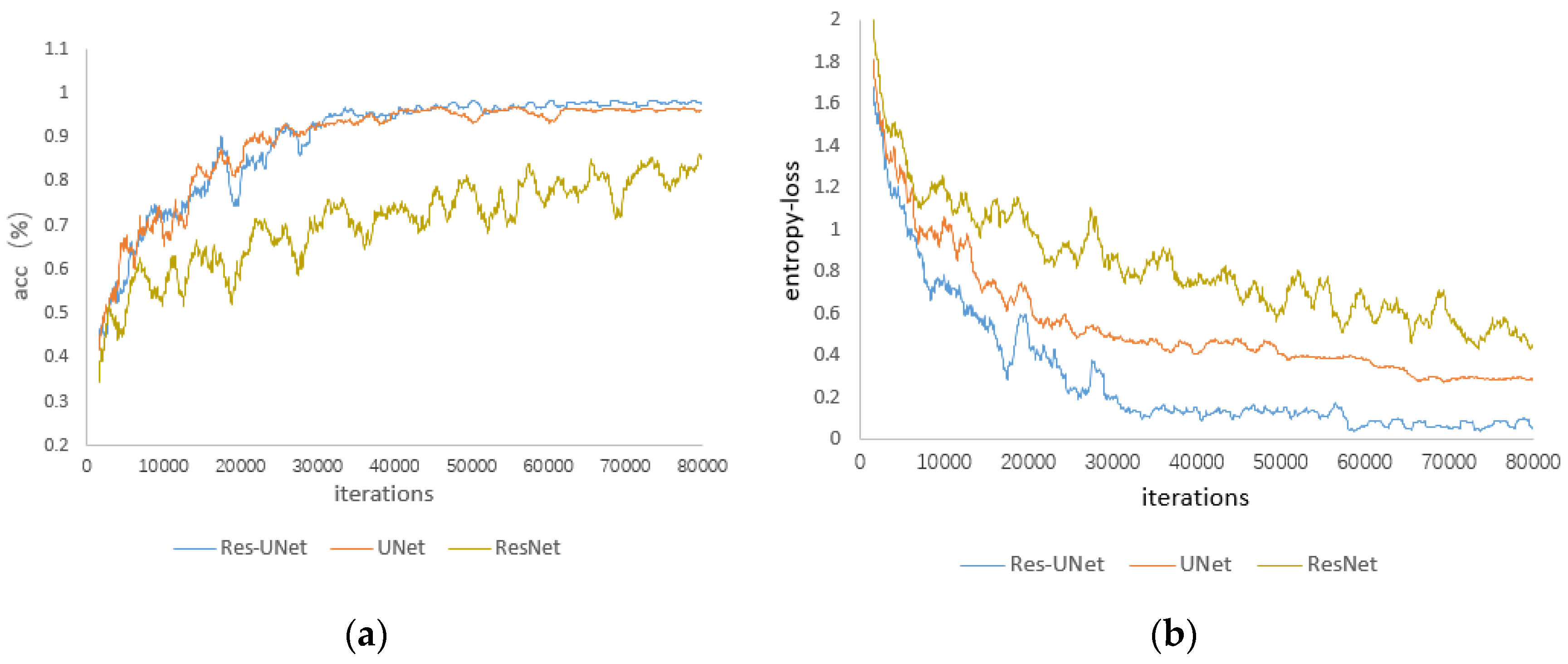
4.2. Comparison of Improved Res-UNet with U-Net and ResNet Networks

The network operation results reveal that Res-UNet obtained the best classification results; i.e., the highest classification accuracy and Kappa coefficient for various tree species, followed by U-Net, with ResNet exhibiting the worst effect. When the ResNet network was used alone, the classification results were fragmented, the edges were rough, the accuracy was low, and severe mixing occurred between tree species. The improved Res-UNet network uses the ResNet residual unit instead of the U-Net network convolution layer, which can extract information at different scales of the image and identify tree species in smaller areas. At the same time, it avoids the gradient degradation problem caused by the deepening of the network layer to obtain the best classification effect. Thus, the proposed Res-UNet can be an effective method for the classification of complex tree species in southern China.

4.3. Comparison of Classification Accuracy for Different Categories

Because various broad-leaved tree species exhibited a sparse distribution, they were classified into other broad-leaved categories. However, due to differences in the characteristics of different broad-leaved tree species, the classification effect was not ideal, even though the accuracy was greatly improved by improving the network. Notably, the planting area of eucalyptus was large and the sample size was sufficient; it exhibited the highest classification accuracy of all tree species. The classification accuracy of Illicium verum is second only to eucalyptus. Its clustered leaves are easily distinguishable from other tree species. Therefore, assuming a sufficient sample size, the improved Res-UNet network can be employed with high-spatial-resolution images to achieve higher tree species classification accuracy.

4.4. Impact of Label Samples on Classification

When using CNNs to classify tree species in remote sensing images, the sample is very important; however, labeling is difficult [47]. For the classification of broad-leaved tree species, the proposed method exhibited relatively low accuracy due to the small sample size. Therefore, for tree species with insufficient sample sizes, the classification accuracy is affected. The issue of sample making is gaining increasing attention from scholars [48]. Some researchers have proposed a method of combining unsupervised learning and semisupervised learning to make samples of each tree species using sparse autoencoders and deep belief networks when testing organic carbon content [49]. It simplifies the production of samples. In future research, we will try to further optimize the network structure to address the small sample problem.

5. Conclusions

In this article, we proposed an improved Res-UNet network for tree classification using high-scoring remote sensing images. This novel method uses the residual unit of ResNet instead of the convolutional layer of the U-Net network; therefore, it can achieve multiscale feature extraction of an image, allowing information to spread from shallow to deep layers while avoiding degradation of network performance. Conditional random fields are used at the output of the network for postclassification processing, which results in smoother tree species boundaries. By using bilinear interpolation instead of deconvolution, the network performance is significantly improved. Experimental results show that, compared with U-Net and ResNet, the improved Res-UNet method can effectively extract the spatial and spectral characteristics of an image. For southern Chinese tree species with small differences in their spectral characteristics, the overall accuracy, average accuracy, and Kappa coefficients were 87.51%, 85.43%, and 84.21%, respectively. The proposed network provides new opportunities for the tree species classification of high-spatial-resolution images.

References

1. Torabzadeh, H.; Leiterer, R.; Hueni, A.; Schaepman, M.E.; Morsdorf, F. Tree species classification in a temperate mixed forest using a combination of imaging spectroscopy and airborne laser scanning. Agric. For. Meteorol. 2019, 279, 107744. [Google Scholar] [CrossRef]
2. Goldblatt, R.; Stuhlmacher, M.F.; Tellman, B.; Clinton, N.; Hanson, G.; Georgescu, M.; Wang, C.; Serrano-Candela, F.; Khandelwal, A.K.; Cheng, W.-H.; et al. Using Landsat and nighttime lights for supervised pixel-based image classification of urban land cover. Remote Sens. Environ. 2018, 205, 253–275. [Google Scholar] [CrossRef]
3. Agüera, F.; Aguilar, F.J.; Aguilar, M.A. Using texture analysis to improve per-pixel classification of very high resolution images for mapping plastic greenhouses. ISPRS J. Photogramm. Remote Sens. 2008, 63, 635–646. [Google Scholar] [CrossRef]
4. Li, Q.; Wong, F.K.K.; Fung, T. Classification of Mangrove Species Using Combined WordView-3 and LiDAR Data in Mai Po Nature Reserve, Hong Kong. Remote Sens. 2019, 11, 2114. [Google Scholar] [CrossRef] [Green Version]
5. Pham, L.T.H.; Brabyn, L.; Ashraf, S. Combining QuickBird, LiDAR, and GIS topography indices to identify a single native tree species in a complex landscape using an object-based classification approach. Int. J. Appl. Earth Obs. Geoinf. 2016, 50, 187–197. [Google Scholar] [CrossRef]
6. Ma, L.; Li, M.; Ma, X.; Cheng, L.; Du, P.; Liu, Y. A review of supervised object-based land-cover image classification. Remote Sens. 2017, 130, 277–293. [Google Scholar] [CrossRef]
7. Zhang, C.; Yue, P.; Tapete, D.; Shangguan, B.; Wang, M.; Wu, Z. A multi-level context-guided classification method with object-based convolutional neural network for land cover classification using very high resolution remote sensing images. Int. J. Appl. Earth Obs. Geoinf. 2020, 88, 102086. [Google Scholar] [CrossRef]
8. Mugiraneza, T.; Nascetti, A.; Ban, Y. WorldView-2 Data for Hierarchical Object-Based Urban Land Cover Classification in Kigali: Integrating Rule-Based Approach with Urban Density and Greenness Indices. Remote Sens. 2019, 11, 2128. [Google Scholar] [CrossRef] [Green Version]
9. Ke, Y.; Quackenbush, L.J.; Im, J. Synergistic use of QuickBird multispectral imagery and LIDAR data for object-based forest species classification. Remote Sens. Environ. 2010, 114, 1141–1154. [Google Scholar] [CrossRef]
10. Immitzer, M.; Atzberger, C.; Koukal, T. Tree Species Classification with Random Forest Using Very High Spatial Resolution 8-Band WorldView-2 Satellite Data. Remote Sens. 2012, 4, 2661–2693. [Google Scholar] [CrossRef] [Green Version]
11. Li, D.; Ke, Y.; Gong, H.; Li, X. Object-Based Urban Tree Species Classification Using Bi-Temporal WorldView-2 and WorldView-3 Images. Remote Sens. 2015, 7, 16917–16937. [Google Scholar] [CrossRef] [Green Version]
12. Wolf, N. Object Features for Pixel-based Classi cation of Urban Areas Comparing Different Machine Learning Algorithms. Photogramm. Fernerkund. Geoinf. 2013, 2013, 149–161. [Google Scholar] [CrossRef]
13. Zhou, J.; Qin, J.; Gao, K.; Leng, H. SVM-based soft classification of urban tree species using very high-spatial resolution remote-sensing imagery. Int. J. Remote Sens. 2016, 37, 2541–2559. [Google Scholar] [CrossRef]
14. Dalponte, M.; Ene, L.T.; Marconcini, M.; Gobakken, T.; Næsset, E. Semi-supervised SVM for individual tree crown species classification. ISPRS J. Photogramm. Remote Sens. 2015, 110, 77–87. [Google Scholar] [CrossRef]
15. Lecun, Y.; Bengio, Y.; Hinton, G. Deep learning. Nature 2015, 521, 436. [Google Scholar] [CrossRef]
16. Chen, Y.; Jiang, H.; Li, C.; Jia, X.; Ghamisi, P. Deep Feature Extraction and Classification of Hyperspectral Images Based on Convolutional Neural Networks. IEEE Trans. Geosci. Remote Sens. 2016, 54, 6232–6251. [Google Scholar] [CrossRef] [Green Version]
17. Makantasis, K.; Karantzalos, K.; Doulamis, A.; Doulamis, N. Deep Supervised Learning for Hyperspectral Data Classification through Convolutional Neural Networks. In Proceedings of the 2015 IEEE International Geoscience and Remote Sensing Symposium (IGARSS), Milan, Italy, 26–31 July 2015; pp. 4959–4962. [Google Scholar]
18. Alipourfard, T.; Arefi, H.; Mahmoudi, S. A Novel Deep Learning Framework by Combination of Subspace-Based Feature Extraction and Convolutional Neural Networks for Hyperspectral Images Classification. In Proceedings of the IGARSS 2018—2018 IEEE International Geoscience and Remote Sensing Symposium, Valencia, Spain, 22–27 July 2018; pp. 4780–4783. [Google Scholar]
19. Hinton, G.; Osindero, S.; Welling, M.; Teh, Y.-W. Unsupervised discovery of nonlinear structure using contrastive backpropagation. Cogn. Sci. 2006, 30, 725–731. [Google Scholar] [CrossRef]
20. Lv, X.W.; Ming, D.P.; Lu, T.T.; Zhou, K.Q.; Wang, M.; Bao, H.Q. A New Method for Region-Based Majority Voting CNNs for Very High Resolution Image Classification. Remote Sens. 2018, 10, 1946. [Google Scholar] [CrossRef] [Green Version]
21. Lu, S.; Wang, B.; Wang, H.; Chen, L.; Linjian, M.; Zhang, X. A real-time object detection algorithm for video. Comput. Electr. Eng. 2019, 77, 398–408. [Google Scholar] [CrossRef]
22. Tong, X.-Y.; Xia, G.-S.; Lu, Q.; Shen, H.; Li, S.; You, S.; Zhang, L. Land-cover classification with high-resolution remote sensing images using transferable deep models. Remote Sens. Environ. 2020, 237, 111322. [Google Scholar] [CrossRef] [Green Version]
23. Guo, W.; Wu, R.; Chen, Y.; Zhu, X. Deep Learning Scene Recognition Method Based on Localization Enhancement. Sensors 2018, 18, 3376. [Google Scholar] [CrossRef] [PubMed] [Green Version]
24. Hua, Y.; Mou, L.; Zhu, X.X. LAHNet: A Convolutional Neural Network Fusing Low- and High-Level Features for Aerial Scene Classification. In Proceedings of the IGARSS 2018—2018 IEEE International Geoscience and Remote Sensing Symposium, Valencia, Spain, 22–27 July 2018; pp. 4728–4731. [Google Scholar]
25. Kilic, E.; Ozturk, S. A subclass supported convolutional neural network for object detection and localization in remote-sensing images. Int. J. Remote Sens. 2019, 40, 1–20. [Google Scholar] [CrossRef]
26. Krizhevsky, A.; Sutskever, I.; Hinton, G. ImageNet Classification with Deep Convolutional Neural Networks. Commun. ACM 2012, 60, 84–90. [Google Scholar] [CrossRef]
27. Russakovsky, O.; Deng, J.; Su, H.; Krause, J.; Satheesh, S.; Ma, S.; Huang, Z.; Karpathy, A.; Khosla, A.; Bernstein, M. ImageNet Large Scale Visual Recognition Challenge. Int. J. Comput. Vis. 2015, 115, 211–252. [Google Scholar] [CrossRef] [Green Version]
28. He, X.; Zou, Z.; He, C.; Zhang, J. High-score image scene classification based on joint saliency and multi-layer convolutional neural network. Acta Geod. Geophys. 2016, 45, 1073–1080. [Google Scholar]
29. Zhang, Y.L.; Yuan, Y.; Feng, Y.C.; Lu, X.Q. Hierarchical and Robust Convolutional Neural Network for Very High-Resolution Remote Sensing Object Detection. IEEE Trans. Geosci. Remote Sens. 2019, 57, 5535–5548. [Google Scholar] [CrossRef]
30. Khan, N.; Chaudhuri, U.; Banerjee, B.; Chaudhuri, S. Graph convolutional network for multi-label VHR remote sensing scene recognition. Neurocomputing 2019, 357, 36–46. [Google Scholar] [CrossRef]
31. Sun, Y.; Huang, J.; Ao, Z.; Lao, D.; Xin, Q. Deep Learning Approaches for the Mapping of Tree Species Diversity in a Tropical Wetland Using Airborne LiDAR and High-Spatial-Resolution Remote Sensing Images. Forests 2019, 10, 1047. [Google Scholar] [CrossRef] [Green Version]
32. Hartling, S.; Sagan, V.; Sidike, P.; Maimaitijiang, M.; Carron, J. Urban Tree Species Classification Using a WorldView-2/3 and LiDAR Data Fusion Approach and Deep Learning. Sensing 2019, 19, 1284. [Google Scholar] [CrossRef] [Green Version]
33. Kim, P. Convolutional Neural Network; Apress: Berkeley, CA, USA, 2017. [Google Scholar]
34. Long, J.; Shelhamer, E.; Darrell, T. Fully Convolutional Networks for Semantic Segmentation. In Proceedings of the Conference on Computer Vision and Pattern Recognition (CVPR), Boston, MA, USA, 7–12 June 2015; pp. 640–651. [Google Scholar]
35. Ronneberger, O.; Fischer, P.; Brox, T. U-Net: Convolutional Networks for Biomedical Image Segmentation. Medical Image Computing and Computer-Assisted Intervention; Springer: Cham, Switzerland, 18 November 2015; pp. 234–241. [Google Scholar]
36. Fang, X.; Wang, G.; Yang, H.; Liu, H.; Yan, L. High Resolution Remote Sensing Image Classification Based on Mean Drift Segmentation and Full Convolutional Neural Network. Laser Optoelectron. Prog. 2017, 55, 446–454. [Google Scholar]
37. Fu, G.; Liu, C.; Zhou, R.; Sun, T.; Zhang, Q. Classification for High Resolution Remote Sensing Imagery Using a Fully Convolutional Network. Remote Sens. 2017, 9, 498. [Google Scholar] [CrossRef] [Green Version]
38. Flood, N.; Watson, F.; Collett, L. Using a U-net convolutional neural network to map woody vegetation extent from high resolution satellite imagery across Queensland, Australia. Int. J. Appl. Earth Obs. Geoinf. 2019, 82, 101897. [Google Scholar] [CrossRef]
39. He, K.; Zhang, X.; Ren, S. Deep Residual Learning for Image Recognition. In Proceedings of the 2016 IEEE Conference on Computer Vision and Pattern Recognition(CVPR), Las Vegas, NV, USA, 27–30 June 2016; pp. 770–778. [Google Scholar]
40. Chu, Z.; Tian, T.; Feng, R.; Wang, L. Sea-Land Segmentation With Res-UNet And Fully Connected CRF. In Proceedings of the IGARSS 2019—2019 IEEE International Geoscience and Remote Sensing Symposium, Yokohama, Japan, 28 July–2 August 2019; pp. 3840–3843. [Google Scholar]
41. Xu, Y.; Wu, L.; Xie, Z.; Chen, Z. Building Extraction in Very High Resolution Remote Sensing Imagery Using Deep Learning and Guided Filters. Remote Sens. 2018, 10, 144. [Google Scholar] [CrossRef] [Green Version]
42. Zhang, P.; Ke, Y.; Zhang, Z.; Wang, M.; Li, P.; Zhang, S. Urban Land Use and Land Cover Classification Using Novel Deep Learning Models Based on High Spatial Resolution Satellite Imagery. Sensing 2018, 18, 3717. [Google Scholar] [CrossRef] [PubMed] [Green Version]
43. Introduction of Gaofeng Forest Farm. Available online: http://www.gaofenglinye.com.cn/lcjj/index_13.aspx (accessed on 28 February 2020).
44. Pang, Y.; Li, Z.; Ju, H.; Lu, H.; Jia, W.; Si, L.; Guo, Y.; Liu, Q.; Li, S.; Liu, L.; et al. LiCHy: The CAF’s LiDAR, CCD and Hyperspectral Integrated Airborne Observation System. Remote Sens. 2016, 8, 398. [Google Scholar] [CrossRef] [Green Version]
45. Smith, P.R. Bilinear interpolation of digital images. Ultramicroscopy 1981, 6, 201–204. [Google Scholar] [CrossRef]
46. Kingma, D.; Ba, J. Adam: A Method for Stochastic Optimization. Comput. Sci. 2014, arxiv:1412.6980. [Google Scholar]
47. Jia, S.; Zhuang, J.Y.; Deng, L.; Zhu, J.S.; Xu, M.; Zhou, J.; Jia, X.P. 3-D GaussianGabor Feature Extraction and Selection for Hyperspectral Imagery Classification. IEEE Trans. Geosci. Remote Sens. 2019, 57, 8813–8826. [Google Scholar] [CrossRef]
48. Fang, B.; Li, Y.; Zhang, H.; Chan, J.C.-W. Collaborative learning of lightweight convolutional neural network and deep clustering for hyperspectral image semi-supervised classification with limited training samples. ISPRS J. Photogramm. Remote Sens. 2020, 161, 164–178. [Google Scholar] [CrossRef]
49. Liu, Y.; Zhou, Y.; Liu, X.; Dong, F.; Wang, C.; Wang, Z. Wasserstein GAN-Based Small-Sample Augmentation for New-Generation Artificial Intelligence: A Case Study of Cancer-Staging Data in Biology. Engineering 2019, 5, 156–163. [Google Scholar] [CrossRef]
Figure 1. Geographical location of Gaofeng Forest Farm Boundary (top left), the CCD orthophoto of Jiepai Field and study area (bottom left), the CCD orthophoto of aerial area (top right), the CCD orthophoto of study area (bottom right).
Remotesensing 12 01128 g001
Figure 2. Workflow for improved U-Net model for tree species classification based on airborne high-resolution images.
Remotesensing 12 01128 g002
Figure 3. Two-level ResNet residual unit (a), Three-level ResNet residual unit (b).
Remotesensing 12 01128 g003
Figure 4. Two residual units used in this study (a,b).
Remotesensing 12 01128 g004
Figure 5. The network structure of UNet.
Remotesensing 12 01128 g005
Figure 6. The network structure of Res-UNet.
Remotesensing 12 01128 g006
Figure 7. Tree species classification results by different classification methods. (a) Ground truth category, (b) the result of ResNet using bilinear interpolation and CRF, (c) the result of U-Net using bilinear interpolation and CRF, (d) the result of Res-UNet using deconvolution and CRF, (e) the result of Res-UNet using bilinear interpolation, and (f) the result of Res-UNet using bilinear interpolation and CRF.
Remotesensing 12 01128 g007
Figure 8. Training accuracy (a) and loss (b) curve of ResNet, UNet, and Res-UNet.
Remotesensing 12 01128 g008
Figure 9. Local map of weakened tree species mixing using CRF.
Remotesensing 12 01128 g009