Estimation of the Lateral Dynamic Displacement of High-Rise Buildings under Wind Load Based on Fusion of a Remote Sensing Vibrometer and an Inclinometer

Abstract

This paper proposes a novel method to estimate the lateral displacement of high-rise structures under wind loads. The coefficient β(x) is firstly derived, reflecting the relation between the structural lateral dynamic displacement and the inclination angle at the height x of a structure. If the angle is small, it is the ratio between the structural fundamental mode shape and its first-order derivative without influence of external loads. Several dynamic experiments of structures are performed based on a laser remote sensing vibrometer and an inclinometer, which shows that the fundamental mode is dominated in the structural displacement response under different types of excitations. Once the coefficient β(x) is curve-fitted by measuring both the structural lateral dynamic displacement and the inclination angle synchronously, the real-time structural lateral displacement under operational conditions is estimated by multiplying the coefficient β(x) with the inclination angle. The advantage of the proposed method is that the coefficient β(x) can be identified by lateral dynamic displacement measured in high resolution by the remote sensing vibrometer, which is useful to reconstruct the displacement accurately by the inclination angle under operational conditions.

1. Introduction

With the development of innovative structural systems and novel construction technology, high-rise buildings with landmarks are emerging all over the world. High-rise buildings must resist vertical gravity load as well as lateral load due to wind and seismic activity. Under operational conditions, the lateral dynamic displacement is a key performance criterion. It must not exceed a certain value so as to avoid damage to brittle building elements. Thus, it is necessary to evaluate the structural dynamic displacement accurately and effectively [1,2,3,4].

Many methods have been proposed to measure the structural dynamic displacement in the field of civil engineering [5]. They can be classified into one of three categories according different measurement systems: The first type of displacement estimation method is based on different sensors directly installed on the structure, such as accelerometer [6,7,8], inclinometer [9], or strain gauge [10,11]. These economical sensors can estimate real-time and continuous dynamic displacement. However, the relative inaccuracy estimation results limit the application of these methods. With regard to accelerometers, the structural displacement can be calculated by double integration of the acceleration response, but it is difficult to assess the displacement accurately due to determination of the integration constant. Meanwhile, inclinometers are widely instrumented on high-rise buildings to assess the lateral displacement, while mainly based on the geometrical relation between the tilt and the lateral displacement instead of dynamic analysis. This will cause a deviation of the real displacement if the high frequency components in the inclination angle signal are not removed. Similarly, dynamic analysis of the strain response is also necessary.

The second category of displacement measurement methods refers to global position systems (GPS) [12,13,14,15,16,17], vision systems [18,19,20,21], radar systems [22,23,24], and laser systems [25,26]. These systems can provide accurate displacement in a noncontact manner. GPS is a promising method for real-time tracking of structural dynamic displacement with centimeter-level accuracy. However, the application of GPS is still limited because of multipath effects, geometry effects of satellites, tropospheric delay, and cycle slips [27,28,29]. Alternatively, vision systems, radar systems, and laser systems have been proposed to measure the structural dynamic displacement. Such systems could be classified as remote sensing (RS) techniques, because the structural displacement is obtained through the analysis of data acquired by devices that are not in contact with the structure under investigation [30,31]. Although RS techniques can provide accurate structural displacement directly with a resolution varying from centimeters to micrometers, these methods are unsuitable in real-time monitoring because it is difficult to achieve a stable reference point in the continuous monitoring campaign when using them. Meanwhile, these systems are subject to ambient influences such as weather conditions. Moreover, they are relatively expensive and thus, it is impossible to leave them on site for continuous monitoring [28,29].

The third category of approaches for displacement measurement relates to fusing data from multiple sensors, such as accelerometer combined with GPS [28,29,32,33], vision system [34], radar system [35], laser system [36], strain gauge [37], or inclinometer [38]. However, the acceleration integration error still exists and influence the displacement estimation [28,29].

This paper proposes a novel method to estimate the lateral displacement of high-rise buildings by fusion of both a laser system and an inclinometer. On the one hand, the laser system can measure the lateral displacement directly with high resolution in a micrometer range, and on the other hand, the force–balance inclinometer can reflect the structural inclination angle continuously. Thus, it is possible to provide real-time structural lateral displacement by fusion of them. The main contributions consist of: (1) The physical relation between the lateral displacement and the inclination angle is derived theoretically. (2) Different dynamic experiments of a steel frame, an 87.7-m-high shearing wall building, and the Kingkey 100 skyscraper are conducted by measuring the lateral displacement and the inclination angle synchronously. It is observed that the fundamental mode dominates in the lateral dynamic displacement under external loads. (3) The curve-fitting method is proposed to determine the coefficient β(x) between the lateral displacement and the inclination angle. Under different external loads, the coefficient β(x) is approximately a constant at the height x of a structure. (4) Thus, the real-time structural lateral displacement under wind loads is estimated by multiplying the fitted constant coefficient β(x) with the inclination angle response.

The current research is divided into 5 sections. In Section 2, the theoretical relation between the lateral displacement and the inclination angle is firstly derived from structural vibration analysis. If the inclination angle is small and only the fundamental mode is considered, the lateral displacement can be expressed as the inclination angle multiplied with a constant coefficient β(x), which is determined by the fundamental mode shape. Subsequently, Section 3 presents a laboratory experiment of a steel frame performed by both inclinometers and laser sensors. It is found that the fundamental mode dominates the structural displacement under different types of excitations. The coefficient β(x) can be curve-fitted by the filtered signals of both the lateral displacement and the inclination angle. Afterward, two dynamic experiments—one of an 87.7-m-high shear wall building and the other of the Kingkey 100 skyscraper—are performed in Section 4. It is observed that the fundamental mode always dominates in the structural vibration under operational conditions. The fitted coefficient β(x) is approximately a constant at the height x of a structure without influences of external excitation. The structural lateral displacement under different loads can be estimated by multiplying the fitted constant coefficient β(x) with the inclination angle. Finally, some conclusions are drawn and future work is discussed.

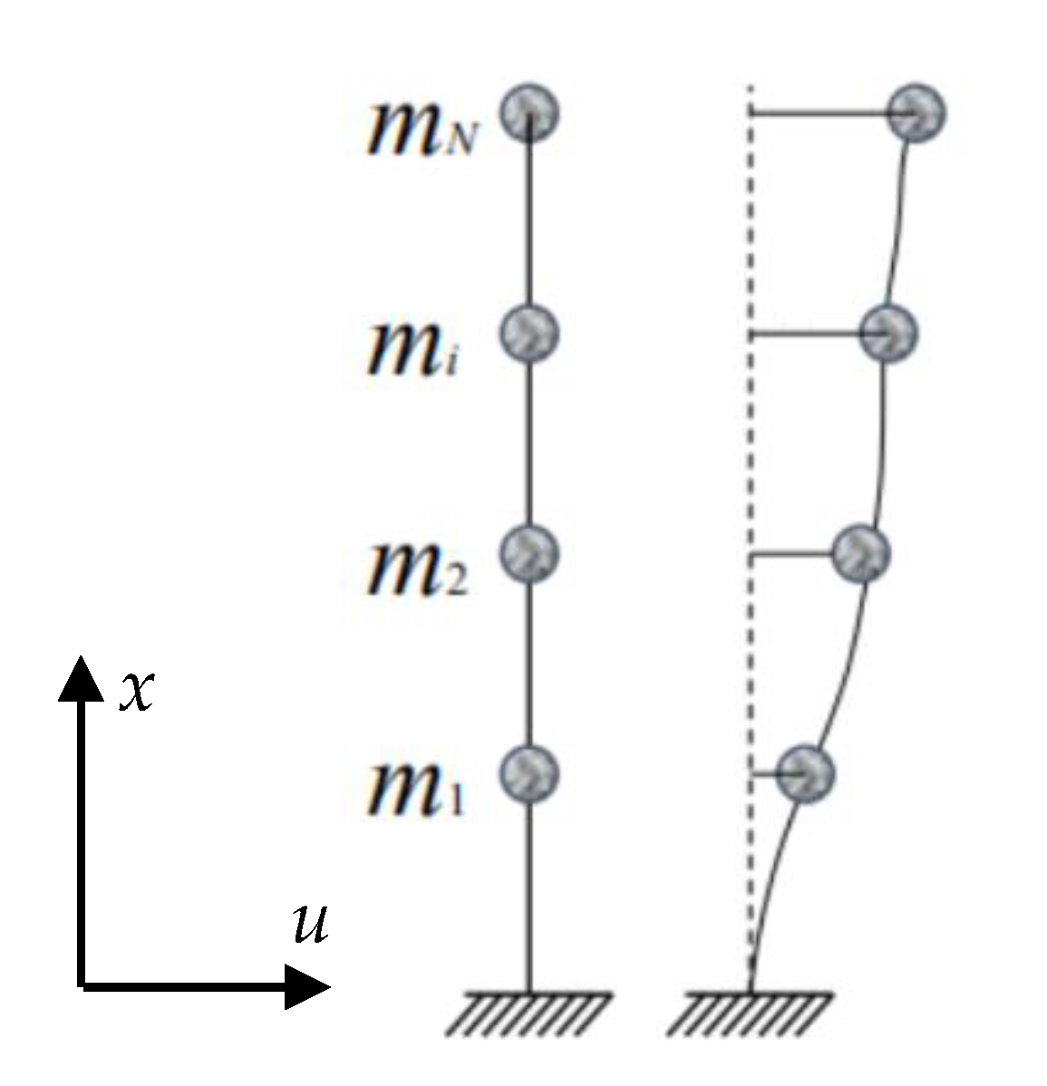
2. Theoretical Derivation

The vibration equation of the structure (Figure 1) under random load is given as

$$M\ddot{u}+C\dot{u}+Ku=P(t)$$

(1)

where M, C, and K are the mass, the damping, and the stiffness matrix of a structure; and $\ddot{u}$, $\dot{u}$, and u are the acceleration, the velocity, and the displacement under random excitation P(t).

The displacement u(x,t) can be solved by separating the vibration mode and the vibration mode coordinate as

$$u(x,t)={\displaystyle \sum _{n=1}^N{\varphi }_n(x)q_n}(t)$$

(2)

where ${\varphi }_n(x)$ is the n^th mode of the structure and x is the height, $q_n(t)$ is the n^th mode coordinate of the structure at time t.

The structural inclination angle $\theta (x,t)$ is obtained by deriving u(x,t) with regard to x:

$$\tan [\theta (x,t)]=\frac{\partial u(x,t)}{\partial x}={\displaystyle \sum _{n=1}^N\frac{\partial {\varphi }_n(x)}{\partial x}}{q}_n(t)$$

(3)

If only the fundamental mode ${\varphi }_1(x)$ is considered and the small-angle $\theta (x,t)$ is approximated (if $\theta <3°,\tan [\theta ]\approx \theta$), Equations (2) and (3) are simplified as

$$u(x,t)\approx {\varphi }_1(x)q_1(t)$$

(4)

$$\tan [\theta (x,t)]\approx \theta (x,t)\approx \frac{\partial {\varphi }_1(x)}{\partial x}{q}_1(t)$$

(5)

Thus, the coefficient β(x) between the structural horizontal displacement u(x,t) and the inclination angle $\theta (x,t)$ is obtained by eliminating $q_1(t)$ as

$$\beta (x)=\frac{u(x,t)}{\theta (x,t)}\approx \frac{{\varphi }_1(x)}{\partial {\varphi }_1(x)/\partial x}$$

(6)

This means that the coefficient β(x) is a constant only associated with the fundamental mode shape ${\varphi }_1(x)$ that reflects the intrinsic property of a structure. In other words, the coefficient β(x) is a constant at the height of x and is not influenced by external loads.

Once β(x) is identified by measurement of both the lateral displacement and the inclination angle simultaneously, the structural lateral displacement under random wind loads can be estimated by the following equation:

$$u(x,t)=\beta (x)\cdot \theta (x,t)$$

(7)

It should be noted that two basic assumptions are always satisfied: (1) the inclination angle $\theta (x,t)$ is small; (2) only the fundamental mode ${\varphi }_1(x)$ is considered. With regard to the inclination angle of a high-rise building, it is quite small under operational conditions, since the largest inclination angle of the top of the Kingkey 100 skyscraper is 1.65° under the super typhoon “Mangkhut” on 16 September 2018. The second assumption is always satisfied for high-rise buildings under wind excitation. The structural displacement responses are divided into two categories, namely along-wind direction and cross-wind direction. With regard to the displacement response along-wind direction, the contribution of the fundamental mode is important and the higher modes can be neglected; regarding to the cross-wind direction, the vortex shedding dominates in the structural displacement except for the fundamental mode. However, the wind tunnel test assists in identifying and avoiding the adverse resonant dynamic response due to vortex shedding [39,40,41].

In this paper, the contribution of the n^th mode to the structural lateral displacement $u(x,t)$ is evaluated by spectral density [42]. A high-rise building is classified as a narrowband system because the area under the response power spectral density (PSD) is highly concentrated near the natural frequencies. Thus, the contribution of the n^th mode C_i is defined as

$$C_i=\frac{R_i}{R}$$

(8)

where R_i is the area of the response PSD near the i^th mode, and R is the whole area of the response PSD.

3. Dynamic Displacement Estimation by Fitting Coefficient β(x)

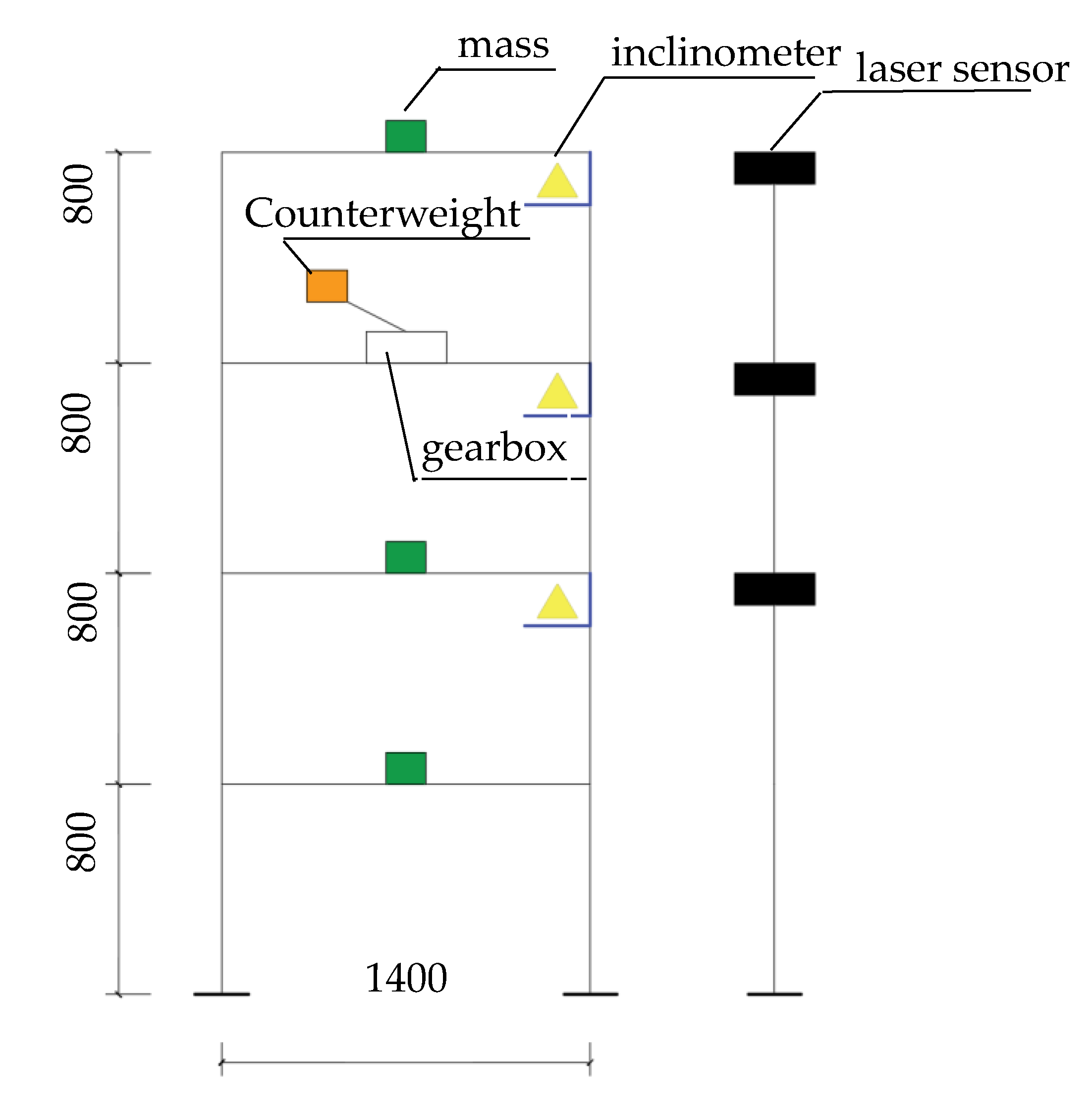
3.1. Laboratoty Dynamic Experiment

In order to verify the feasibility of the proposed method, a four-story steel frame was constructed in the laboratory. Figure 2 shows a diagram of the steel frame and its dimensions. A loading system was installed on the third story, consisting of a gearbox, a rotation counterweight, and an inverter (Tesech E380A), which provides periodical excitation with adjustable rotation frequency and thus, different lateral vibration amplitudes of the steel frame are realized. Additional mass was placed on the other three stories so that the masses of the different stories were equal.

The measurement system was composed of three laser sensors (micro-epsilon, optoNCDT 1700) and three force–balance inclinometers (Jewell LCF100). The laser sensors were fixed on a steel pillar parallel to the steel frame so that the lateral vibration corresponding to the inclinometers could be acquired. Furthermore, a data acquisition system was developed with NI 9234 and NI 9188 hardware and LabVIEW software. In the dynamic experiment, four types of external excitation were applied on the steel frame: random excitation, and excitation with 2, 5, and 10 rad/s. The lateral displacement and rotation angle responses on the second, third and fourth stories were acquired simultaneously by a laser sensor and an inclinometer, respectively. The sampling frequency was 20 Hz and the sampling length was 4 min.

Meanwhile, the finite element (FE) model was also developed with 500 shell elements and four mass elements, as shown in Figure 3. The boundary condition was simulated by 12 spring elements. The frequencies calculated by the FE model and estimated by the dynamic experiment are listed in

Table 1. Comparison of the frequencies simulated by the FE model and estimated by the dynamic experiments.

Mode Order	Frequency (Hz)
	FE Model	Displacement	Inclination Angle
1	1.04	0.97	0.98
2	3.82	3.52	3.52
3	7.63	6.90	7.01

. It is found that the frequencies identified by the displacement response are quite similar to those estimated by the angle response; however, both of them are smaller than the simulation results.

3.2. Fitting Coefficient β(x) and the Dynamic Displacement Estimation

Figure 4a,b plots the original lateral displacement and the inclination angle on the fourth story, measured by both the laser sensor and the inclinometer. The corresponding filtered responses are also overlapped. It is observed from Figure 4b that the original inclination angle varies from −0.019° to 0.018° and the inclination angle is quite small. Thus, tanθ(x,t) in Equation (5) is approximately equal to θ(x,t); meanwhile, inspection of the corresponding power spectra density (PSD) in Figure 4c shows that the first mode vibration component dominates in the displacement response. Conversely, Figure 4d demonstrates that the second and third modes also make a significant contribution to the inclination angle response. It is also evidenced by Figure 4a,b that more fluctuations are observed in the original inclination angle response than those in the displacement signal, highlighting the influences of vibration in the higher modes.

Table 2. The contribution of the i^th mode order calculated by both the lateral displacement and the inclination angle.

External Excitation	Mode Order
	1st		2nd		3rd		The Rest
	Displacement	Angle	Displacement	Angle	Displacement	Angle	Displacement	Angle
Random vibration	96.8	85.4	2.5	7.2	0.6	5.7	0.1	1.7
2 rad/s	96.4	72.5	2.9	12.3	0.6	9.6	0.1	5.6
5 rad/s	96.2	78.5	3.1	8.8	0.6	6.8	0.1	5.9
8 rad/s	95.1	75.4	3.1	9.5	1.5	8.9	0.3	6.1

lists the contribution of the i^th mode calculated by both the displacement and the angle responses. It can be observed that the contribution of the first mode of the displacement is over 95%, regardless of the different types of external excitations, indicating that the vibration of the first mode always dominates in the displacement signal. On the contrary, the contribution of the first mode of the angle signal is nearly less than 86%, suggesting the influences of the vibration contribution of higher modes in the original angle signal. It is also evidenced by Figure 4a,b that the inclination angle signal has more fluctuations than the lateral displacement.

Since the fundamental mode vibration component dominates in the displacement response, it is reasonable to filter the displacement signal by only retaining the contribution of the fundamental mode. As show in Figure 4e,f, the corresponding PSD curve of the lateral displacement and angle responses (Figure 4a,b) around the fundamental frequency (0.97 Hz) is retained and the rest of the frequency curve is set to zero. The displacement and angle signals can be filtered by performing inverse-Fast Fourier Transformation (IFFT) based on the PSD curve in Figure 5a,b. Only the contribution of the fundamental mode was considered and the influence of the rest of the frequency components were filtered.

It is noticed that the filtered displacement signal is similar to the original displacement response in Figure 4a, while the obvious fluctuations of the original angle signal in Figure 4b are removed in the filtered angle signal, which varies only from −0.007° to 0.007°. This means that the vibration components in the higher modes of angle response are well filtered.

Figure 5a displays the filtered lateral displacement and the filtered angle responses. The similar fluctuations in these two signals are noted, though the vibration amplitudes are different. A similar phenomenon is also observed in the corresponding PSD curves, as shown in Figure 4e,f and Figure 5b.

According to Equation (6), the coefficient β(x) can be estimated by least-square fitting the filtered angle response to the filtered displacement signal. Afterwards, the displacement curve can be achieved by multiplying the coefficient β(x) with the angle response in the time domain based on Equation (7). In Figure 5c, the original lateral displacement measured by the laser sensor, the filtered displacement, and the estimated displacement are plotted in blue, red, and black, respectively. It is observed that the estimated displacement by angle response is nearly the same as the filtered displacement, and quite similar to the original displacement measured directly by the laser sensor. Meanwhile, the PSD of the filtered lateral displacement can also be produced by multiplying the filtered angle response with the coefficient β(x), as shown in Figure 5d.

Table 3. Comparison of the maximum value between the displacement measured by the laser sensor and the displacement estimated by multiplying the inclination angle with the coefficient β(x).

External Excitation	Original Displacement	Coefficient β(x)	Estimated Displacement by Multiplying β(x) with the Inclination Angle	Difference (%)
Random	4.89	23.75	4.66	4.7
2 rad/s	0.039	24.54	0.038	2.5
5 rad/s	0.050	24.12	0.052	3.8
8 rad/s	0.376	23.51	0.377	0.2

compares the maximum values of both the original displacement measured by the laser sensor and the displacement estimated by multiplying the angle with coefficient β(x) under different types of external excitations. It is found that the differences are in the range of 0.2%–4.7%. This implies that the structural lateral displacement can be accurately estimated by the coefficient β(x) and the angle responses.

Table 4. Comparison of the coefficient β(x) fitted by both the lateral displacement and the inclination angle, as well as calculated by the finite model.

Story	External Excitation	Coefficient β(x)	Mean Value	FE Model
2	Random	23.14	23.08	24.09
	2 rad/s	23.55
	5 rad/s	22.62
	8 rad/s	23.03
3	Random	23.86	23.34	24.16
	2 rad/s	23.15
	5 rad/s	23.18
	8 rad/s	23.16
4	Random	23.75	23.98	24.27
	2 rad/s	24.54
	5 rad/s	24.12
	8 rad/s	23.51

shows the fitted coefficient β(x) of the different stories under different types of external excitations. It is interesting to note that the coefficient β(x) varies slightly with the height x and can be approximated as a constant regardless of the external excitation. Such a phenomenon may be explained by Equation (6). At the same time, the coefficient β(x) can also be calculated by the finite element model. Both are close to the mean value of the fitted coefficient β(x) at the height x, which is further validated by the fact that that the coefficient β(x) is associated with the fundamental mode shape if the inclination angle is assumed to be small (Equations (3)–(6)).

4. Dynamic Displacement Estimation of High-Rise Buildings

In this section, the dynamic experiments are performed on both a shear wall high-rise building (87.7 m) and a super tall skyscraper (Kingkey 100, 441.8 m). The coefficient β(x) is curve-fitted by both the lateral displacement and the inclination angle. Then, the real-time structural displacement is estimated by multiplying the coefficient β(x) and the inclination angle according to Equation (7).

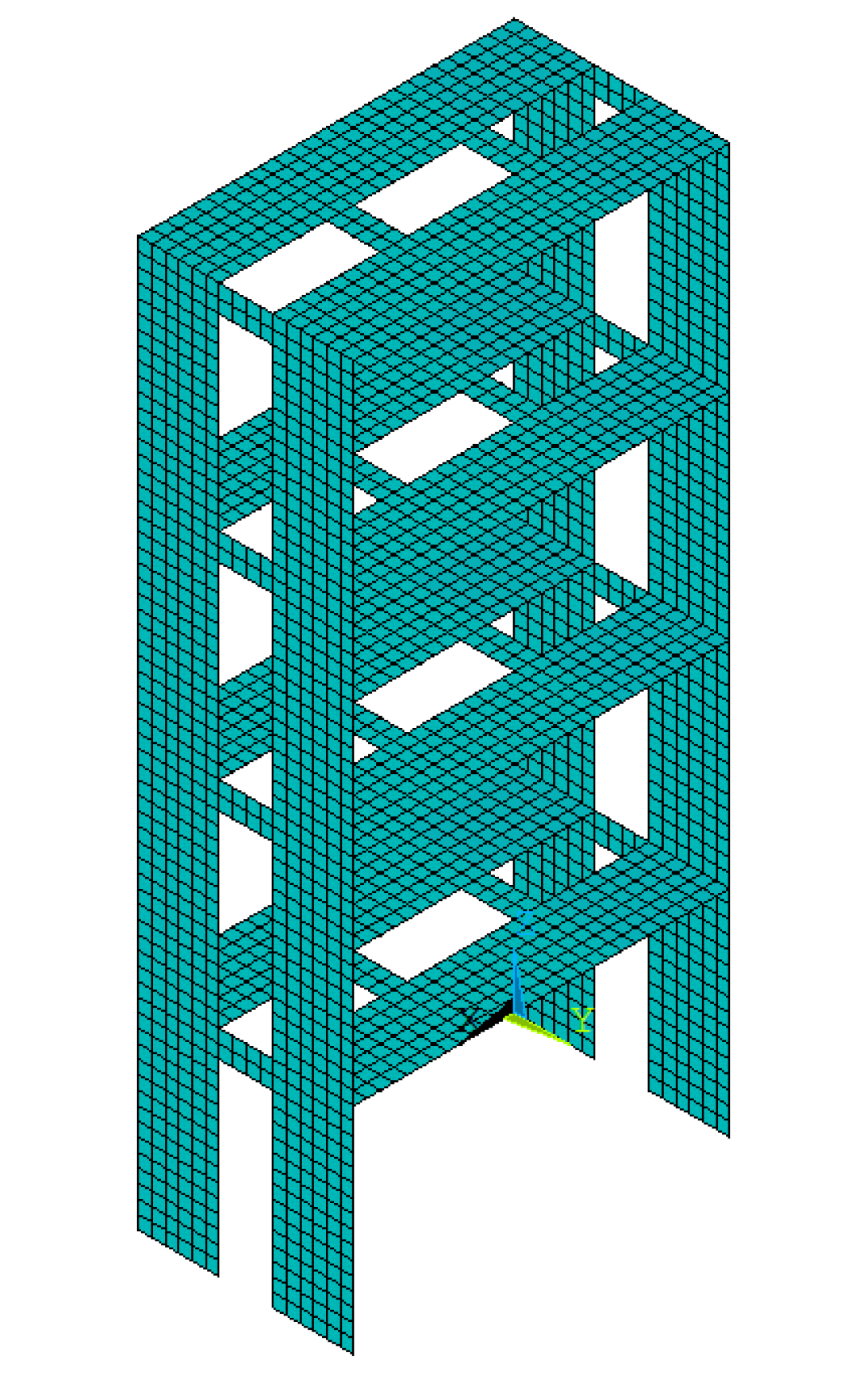
4.1. Dynamic Displacement Estimation a Shear Wall High-Rise Building

The shear wall high-rise building used in this experiment is one of the dormitories on the campus of the Harbin Institute of Technology (Shenzhen), as shown in Figure 6a. Figure 7 shows the synchronous measurement system, which consists of a remote sensing vibrometer and an inclinometer, responsible for acquiring the structural displacement and the inclination angle, respectively. Both of them were synchronized by a GPS clock so that the displacement and inclination angle can be measured simultaneously. The remote sensing vibrometer (Polytec, RSV150) was placed 234.91 m away from the building in order to acquire the structural displacement response on both the 14th floor (44.8 m) and the 23rd floor (74.5 m), as shown in Figure 8. It is also interesting to note a laser point in Figure 6a. The inclinometer (Jewell LCF100) was fixed on the wall near the laser point. A data acquisition system was developed with NI 9234 and NI 9171 hardware and LabVIEW software, and six dynamic experiments were performed with a 100 Hz sampling frequency and a 5 min sampling length.

Then, an FE model was constructed (Figure 6b), and a modal experiment based on a distributed acceleration measurement system was conducted via the synchronous acquisition system. The detailed results can be consulted in [43].

It should be emphasized that the displacement measured by the remote sensing vibrometer is along the laser direction. It is composed of both lateral and vertical vibration components, as follows:

$$u_a=u_l\cos \alpha +u_v\sin \alpha$$

(9)

where α is the angle between the laser direction and the horizontal direction; u_a is the displacement along the laser direction; and u_l and u_v are the structural lateral and vertical vibrations.

With regard to a high-rise building, the vertical vibration under wind loads is omitted, and Equation (9) is expressed as

$$u_a\approx u_l\cos \alpha$$

(10)

The dynamic test was conducted in 18 June 2019. The wind speed within the first 10 min of each hour is plotted in Figure 9, reflecting the random wind loads in the dynamic experiment.

Figure 10a,b shows the original lateral displacement and the inclination angle acquired from both the remote sensing vibrometer and the inclinometer from the 23rd floor. The inclination angle varies from −0.02° to 0.02°, satisfying the assumption of a small inclination angle in Equation (5). The corresponding PSDs are plotted in Figure 10c,d.

Table 5. Comparison of the frequencies simulated by the FE model and estimated by dynamic experiments.

Mode Order	Frequency (Hz)
	FE Model	Modal Identification
		Displacement	Inclination Angle	Acceleration
1	0.72	0.70	0.70	0.69
2	3.38	3.16	3.25	3.15
3	7.19	6.74	6.76	6.87
4	11.14	11.19	10.69	11.12

lists the frequencies calculated by the numerical model, as well as estimated by the lateral displacement, the inclination angle, and the acceleration responses. It is noted that the numerical results are slightly larger than the identified frequencies. Moreover, it is evidenced from

Table 6. The contributions of different modes of both lateral displacement and inclination angle.

Experiment Number	Mode Order
	1		2		3		The Rest
	Displacement	Angle	Displacement	Angle	Displacement	Angle	Displacement	Angle
1	96.9	85.4	1.8	11.0	1.1	3.4	0.2	0.2
2	95.7	81.1	2.3	12.3	1.9	6.5	0.1	0.1
3	95.5	78.6	2.9	13.2	1.4	8.9	0.1	0.3
4	97.1	79.1	1.5	12.2	1.3	8.6	0.1	0.1
5	96.5	84.0	1.8	11.9	1.3	4.0	0.4	0.1
6	95.4	76.4	2.4	14.2	1.9	9.2	0.3	0.2

that the contribution of the fundamental mode is larger than 95%, implying that it dominates the lateral displacement response of the shear wall high-rise building under operational conditions; in contrast, the fundamental mode of the inclination angle makes less contribution to the angle response. Thus, only the first mode of the inclination angle was used to estimate the lateral displacement and the other frequency components were ignored.

Figure 11a shows the filtered displacement and the filtered inclination angle by only retaining the PSD around the first mode, as shown in Figure 11b. On the basis of Equation (6), the coefficient β(x) can be fitted by the filtered displacement and the filtered inclination angle. Subsequently, the displacement can be estimated by multiplying the fitted coefficient β(x) and the inclination angle, which is plotted in black in Figure 11c. Figure 11c also displays the original displacement measured by the remote sensing vibrometer and the filter displacement in blue and red, respectively. It is observed that all three curves are nearly same, suggesting that the lateral displacement is accurately estimated by the fitted coefficient β(x) and the inclination angle on the basis of Equation (7). It can be further validated by the fact that the PSDs of both the original and the estimated lateral displacement are similar, as shown in Figure 11d.

Table 7. Comparison of the maximum value between the displacement measured by the remote sensing vibrometer (RSV) and the displacement estimated by multiplying the inclination angle with the coefficient β(x).

Floor	Method	Displacement (mm)
		1	2	3	4	5	6
14	Original displacement	0.302	0.261	0.315	0.265	0.688	0.421
	Coefficient β(x) and inclination angle	0.300	0.260	0.303	0.232	0.693	0.413
	Difference (%)	0.6	0.4	3.8	2.5	0.7	1.9
23	Original displacement	0.530	0.646	0.499	0.774	1.614	0.939
	Coefficient β(x) and Inclination angle	0.536	0.636	0.495	0.758	1.600	0.934
	Difference (%)	1.1	1.5	0.8	2.1	0.8	0.5

compares the maximum values of both the original lateral displacement and the displacement estimated by the angle and the coefficient β(x) under operational conditions. It is found that the differences between them fall in the range of 0.4%–3.8%. This indicates that the lateral displacement of a shear wall high-rise building can be accurately estimated by the coefficient β(x) and the angle responses.

It is interesting to note from

Table 8. Comparison of the coefficient β(x) fitted by both the lateral displacement. The inclination angle, as well as calculated by the finite model.

Floor	Experimental Group	Fitted β(x) Value	Mean	FE Model
14	1	482.88	483.70	500.24
	2	487.84
	3	481.44
	4	486.40
	5	479.16
	6	481.22
23	1	493.92	488.85	510.05
	2	490.42
	3	489.12
	4	484.64
	5	489.92
	6	488.16

that the coefficient β(x) at a certain floor varies slightly and can be regarded as a constant without influences of wind speed. At the same time, the coefficient β(x) is calculated by the finite element model according to Equation (6), which is slightly larger than the mean value of the fitted coefficient β(x)at the height x. It may be further validated that the coefficient β(x) is associated with the fundamental mode shape and is not influenced by the externa loads, as described in Equation (6).

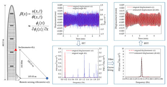
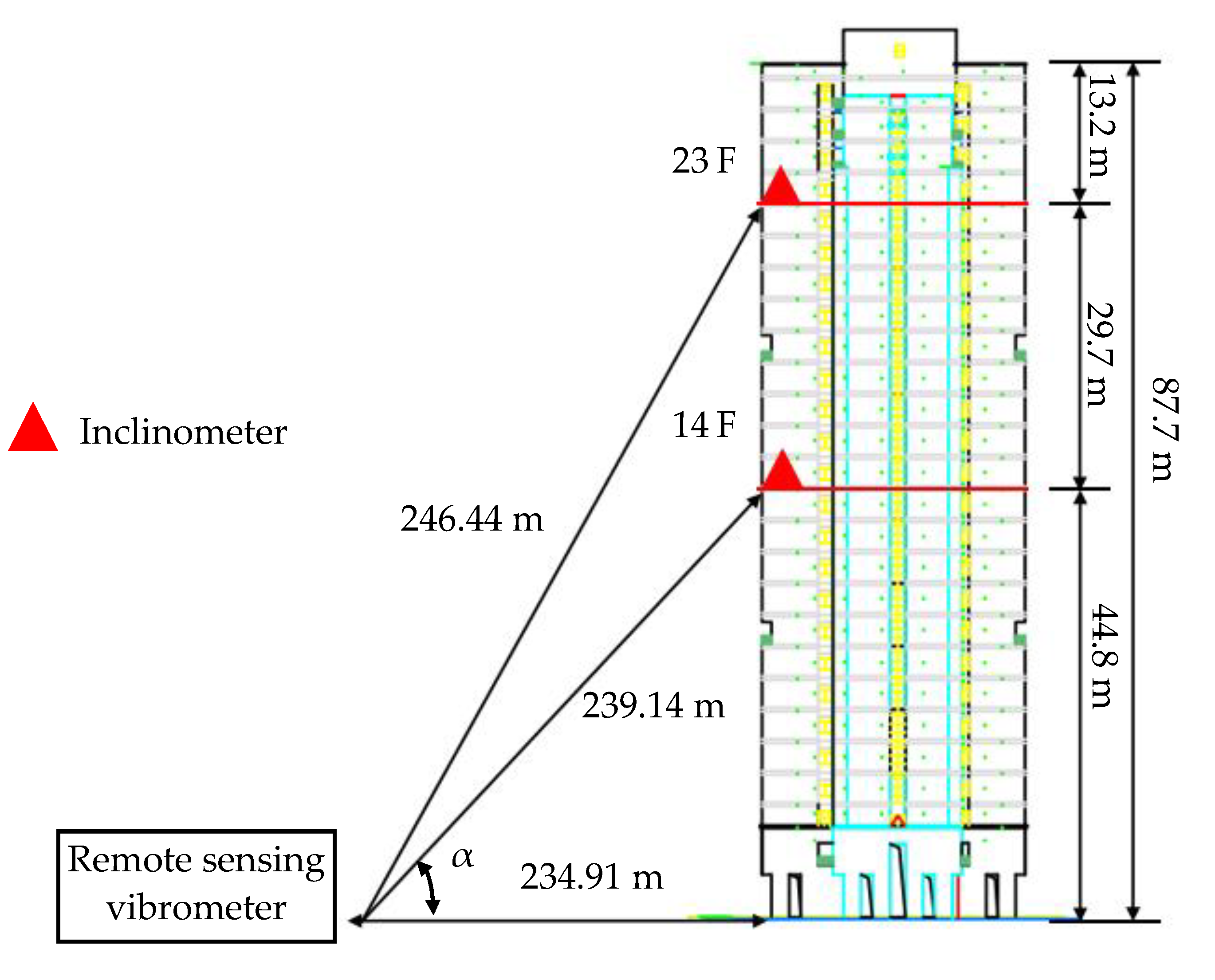
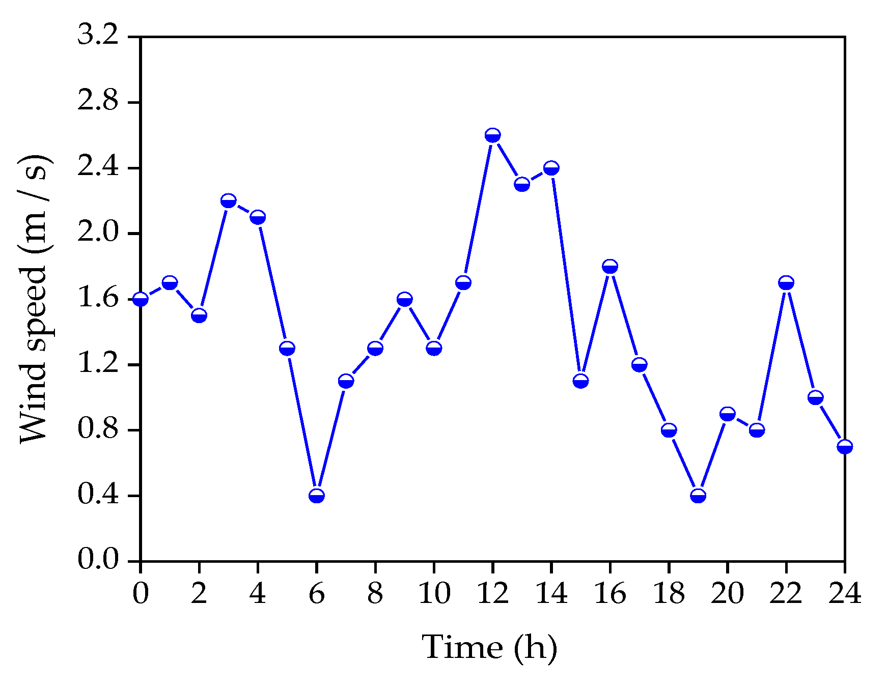
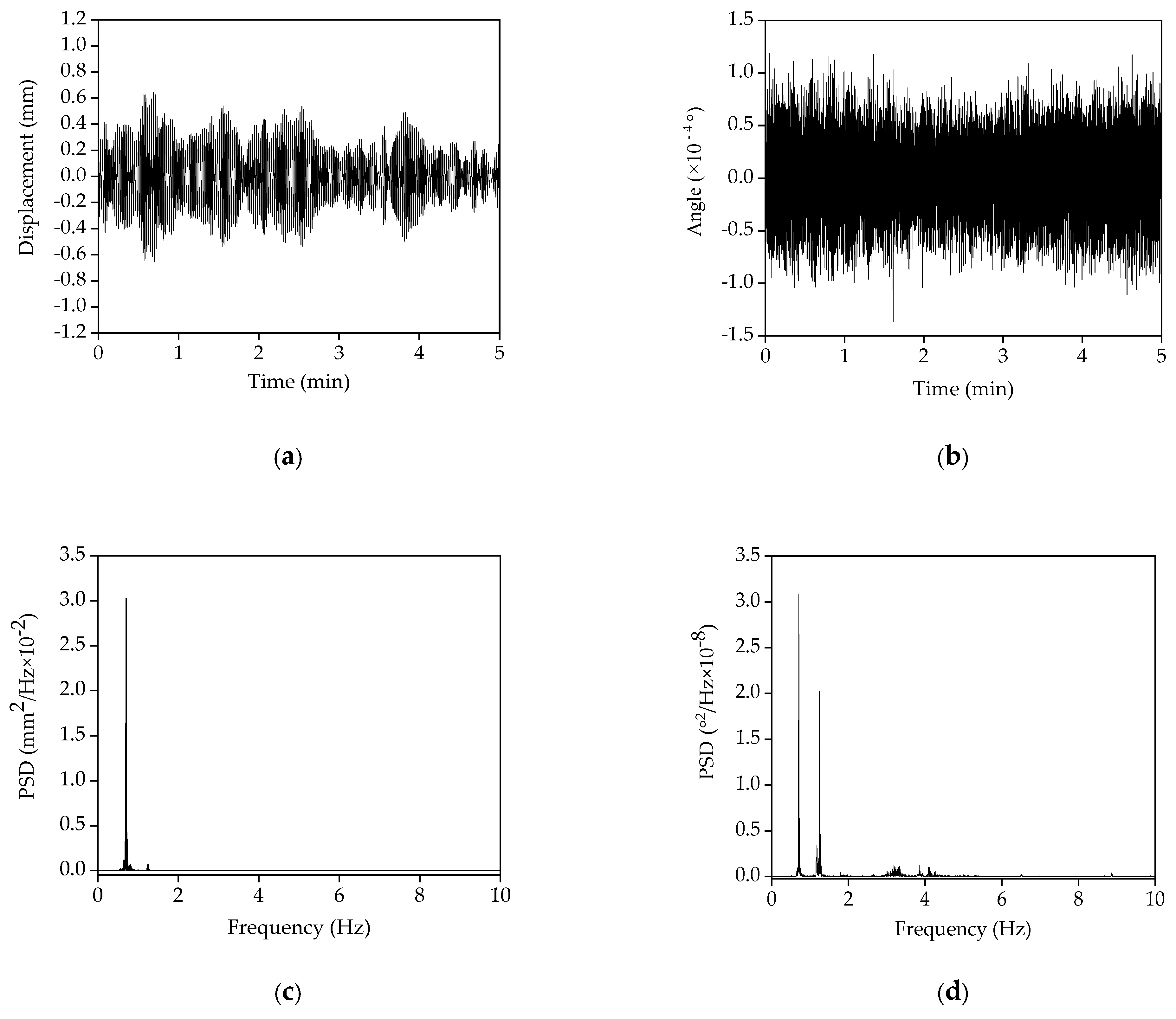
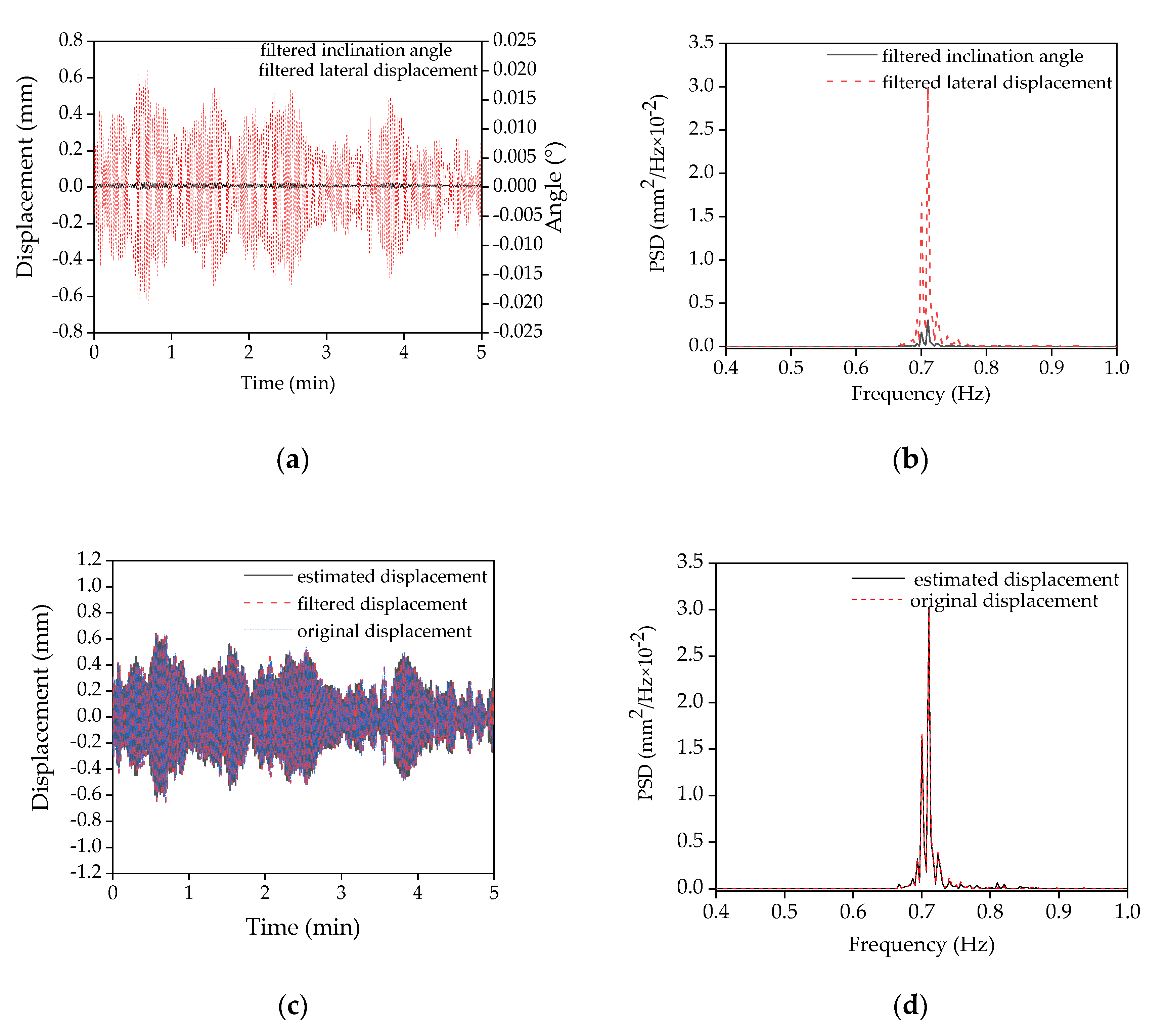
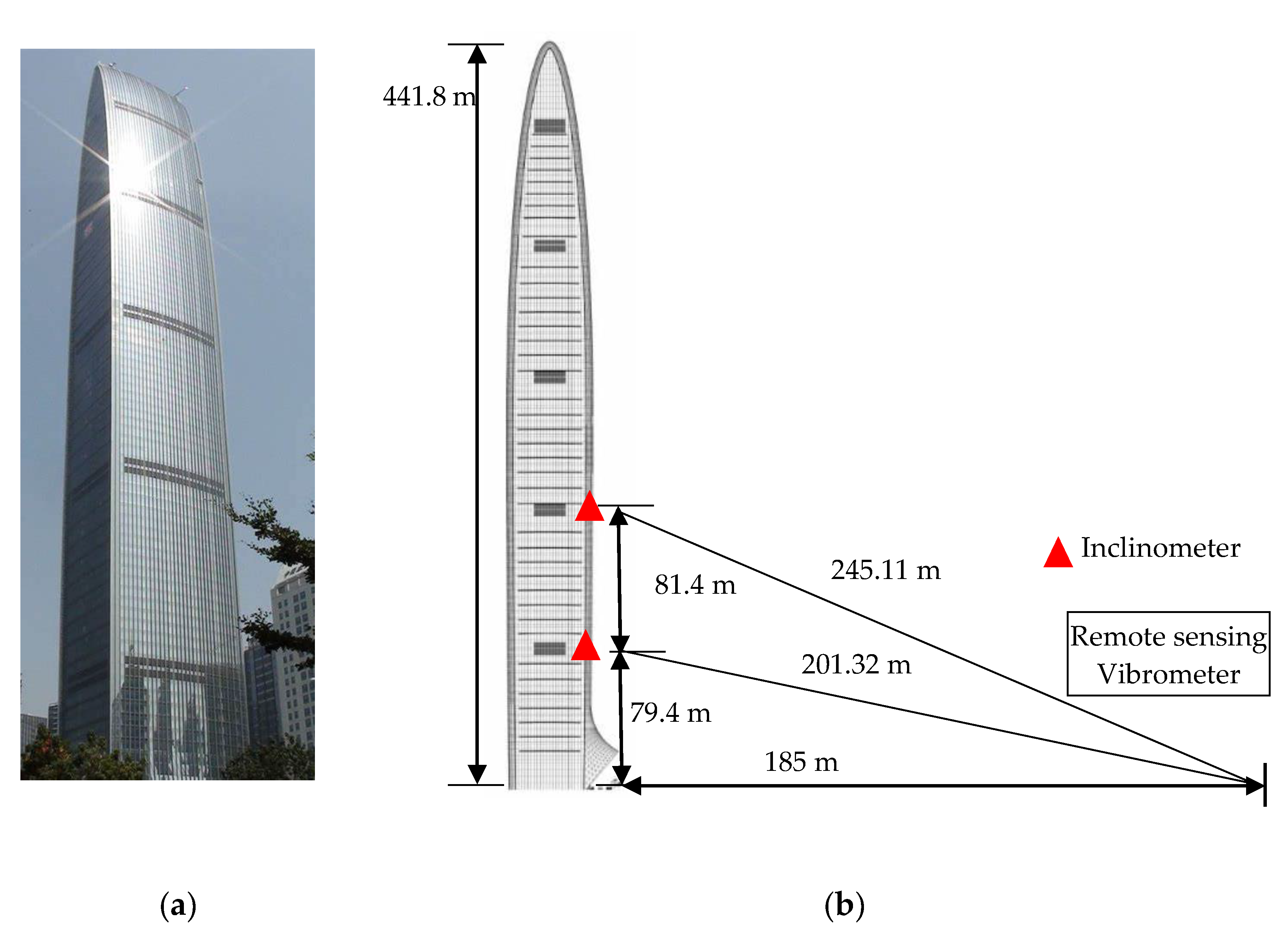
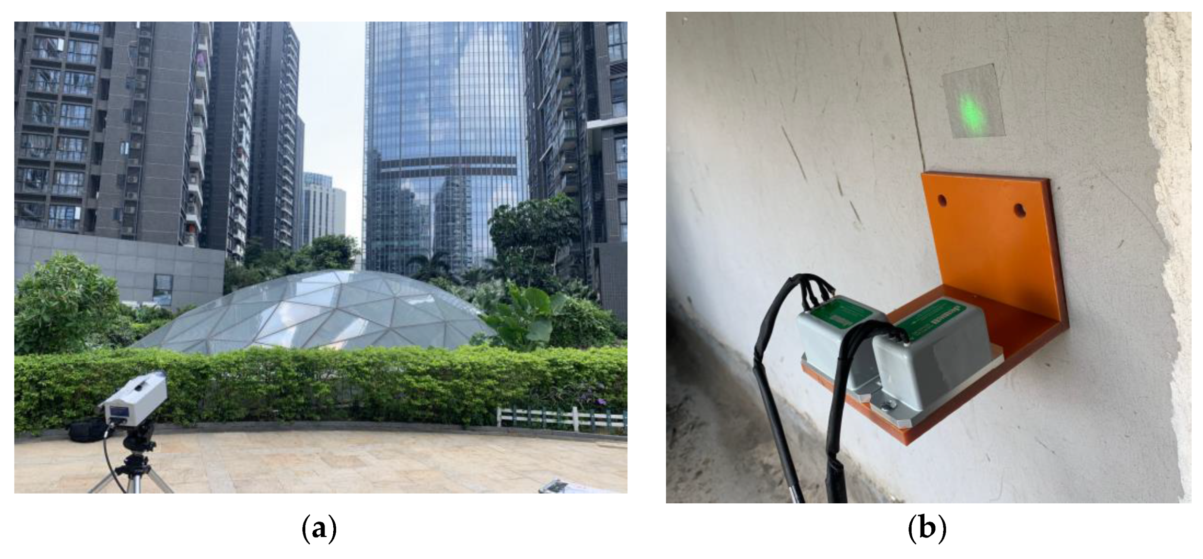
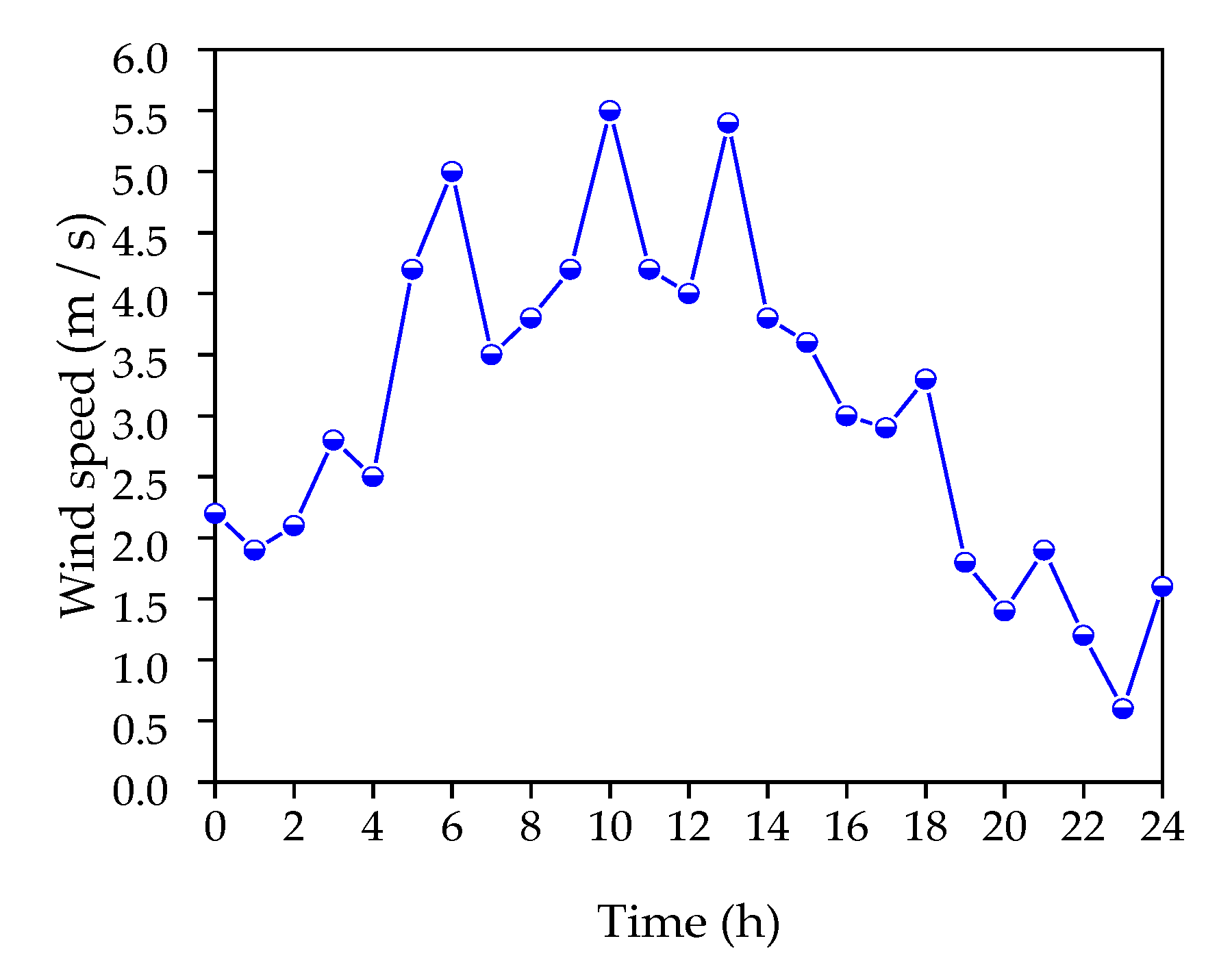
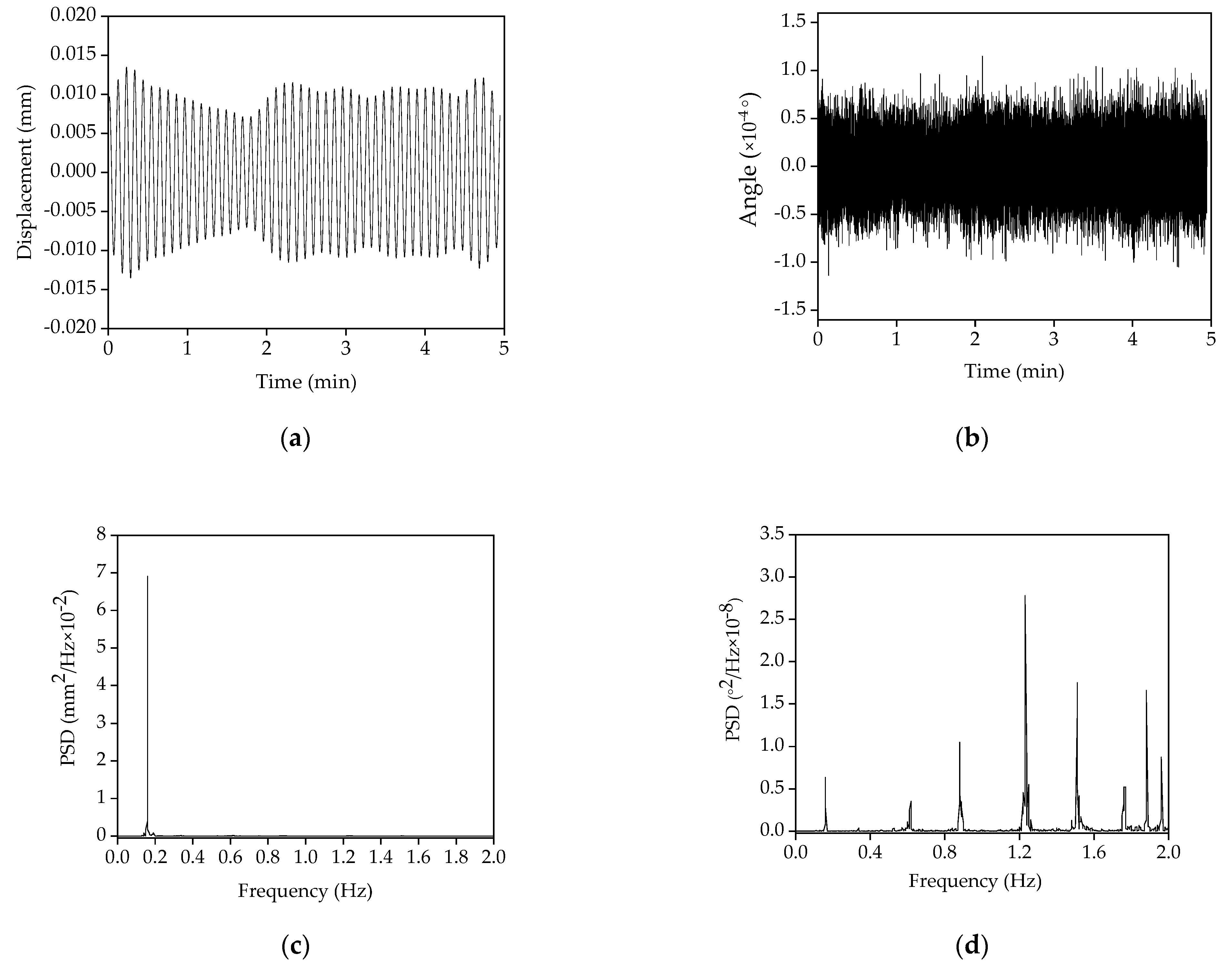
4.2. Dynamic Displacement Estimation of the Kingkey 100 Skyscraper

The Kingkey 100 skyscraper is a 441.8-m-high building with 100 floors, ranking as the second-highest building in Shenzhen, China (Figure 12). The structural dynamic property was thoroughly investigated in [43]. In this paper, a dynamic experiment was performed on the basis of the synchronous measurement system on 18, October 2019. The vibrometer was placed 185 m away from the foot of the Kingkey 100 building (Figure 12b and Figure 13a). The force–balance inclinometer (Jewell LCF100) was installed on the column of the 18th floor (79.4 m) and the 37th floor (160.8 m) respectively, as shown in Figure 12b and Figure 13b. The green laser spot from the remote sensing vibrometer is also captured in Figure 13b. The displacement and inclination angle responses were acquired simultaneously with a sampling frequency of 20 Hz and a sampling length of 5 min. Figure 14 plots the mean wind speed in the first 10 min of each hour on 18 October 2019.

Figure 15a,b shows the original lateral displacement and inclination angle. They were measured by the remote sensing vibrometer and the inclinometer from the 18th floor. The inclination angle varies from −0.002° to 0.002° under wind excitation, which is approximately regarded as a small inclination angle in Equation (5). Figure 15c,d displays the corresponding PSDs.

Table 9. Comparison of the frequencies simulated by the finite model and estimated by dynamic experiments.

Mode Order	Frequency (Hz)
	Displacement	Inclination Angle	Acceleration
1	0.159	0.160	0.155
2	0.583	0.608	0.596
3	0.881	0.889	0.865
4	1.235	1.239	1.204
5	1.755	1.751	1.731

shows the frequencies estimated by the lateral displacement, the inclination angle, and the acceleration responses. Moreover, it is evidenced from

Table 10. Contribution of the different modes of both the lateral displacement and the inclination angle (18th floor).

Experiment Number	Mode Order
	1		2		The Rest
	Displacement	Angle	Displacement	Angle	Displacement	Angle
1	96.1	20.3	2.8	9.5	1.1	70.2
2	96.8	23.9	2.3	10.1	2.0	66.0
3	95.5	26.6	2.9	4.7	1.5	67.7

that the contribution of the fundamental mode of the lateral displacement response is larger than 95.5%. This means that the first mode makes the main contribution to the lateral displacement response of the skyscraper under operational conditions. On the contrary, the fundamental mode of the inclination angle makes less than 26.6% contribution to the angle response. Thus, only the first mode of the inclination angle was retained to estimate the lateral displacement according to Equation (6).

As described in the above sections, the coefficient β(x) can be fitted by the filtered displacement and the filtered inclination angle. Figure 16a shows the filtered displacement and the filtered inclination angle by only retaining the PSD curve near the fundamental mode (Figure 16b). Figure 16c also shows the estimated displacement, the original displacement, and the filter displacement curves. It is found that all three lines are nearly same, suggesting that the lateral displacement can be estimated by the fitted coefficient β(x) and the inclination angle on the basis of Equation (7). The very similar PSD curves in Figure 16d imply that the structural lateral displacement can be reproduced by multiplying the fitted coefficient β(x) with the inclination angle in the frequency domain.

It is worth noting in Figure 17, that the maximum inclination angle at the top of the Kingkey 100 building is only 1.65° under the typhoon “Mangkhut” on 16 September 2018. It is interesting to note that the first vibration mode always makes a significant contribution to the angle responses. Such an observation may suggest that the basic assumptions of the proposed method are always satisfied under operational conditions.

Table 11. Comparison of the maximum value between the displacement measured by the RSV and multiplying the estimated by inclination angle with the coefficient β(x).

Floor	Method	Displacement (mm)
		1	2	3
18F	Original lateral displacement	0.0143	0.0081	0.0079
	Coefficient β(x) and Inclination angle	0.0141	0.0077	0.0082
	Difference (%)	1.4	4.9	3.8
37F	Original lateral displacement	0.0261	0.0360	0.0310
	Coefficient β(x) and Inclination angle	0.0253	0.0365	0.0324
	Difference (%)	3.1	1.4	4.5

lists the peak values of both the original lateral displacement and the estimated displacement. The differences between them vary from 1.4% to 4.9%. This means that the lateral displacement of the Kingkey 100 super high-rise building can be accurately estimated by the fitted coefficient β(x) and the angle responses.

It is also noticed from

Table 12. The coefficient β(x) fitted by both the lateral displacement and the inclination angle.

Floor	Fitted β(x) Value	Mean
37F	576.9	575.1
	578.5
	569.8
18F	589.4	581.7
	578.3
	577.5

that the fitted coefficient β(x) at a certain floor varies slightly and can be approximated as a constant. It is further validated that the β(x) is not influenced by external wind load.

5. Conclusions and Future Works

In this paper, the structural lateral displacement of high-rise buildings under operational conditions was estimated by a fusion of both the remote sensing vibrometer and the inclinometer. If the first vibration mode component is considered and the inclination angle is small, the lateral displacement can be expressed as the product between the inclination angle and a linear constant coefficient β(x). A series of dynamic experiments on a steel frame, a high-rise building, and the Kingkey 100 skyscraper were conducted. It was found that the first vibration mode component always dominates the lateral displacement. Meanwhile, the structural inclination angle is less than 1.65°, even under typhoon weather. The two basic assumptions of the proposed method are always satisfied under operational conditions. The experimental results show that the coefficient β(x) is approximated as a constant at the height x of a structure, regardless of the external excitations. The difference between the measured lateral displacement and the estimated displacement is less than 4.9%.

Due to the limitations of the current remote sensing technology, the maximum measurement distance of the high-accuracy vibrometer is less than 300 m. This means that the coefficient β(x) beyond the scope has to be determined by numerical analysis. In the future, a fine FE model and a synchronous monitoring system of the inclination angle will be developed so that the real-time monitoring of the lateral displacement of the super high-rise buildings under operational condition can be realized.

References

1. Au, S.K.; Zhang, F.L. Top field observations on modal properties of two super tall buildings under strong wind. J. Wind. Eng. Ind. Aerodyn. 2012, 101, 12–23. [Google Scholar] [CrossRef]
2. Zhang, F.L.; Xiong, H.B.; Shi, W.X.; Ou, X. Structural health monitoring of a super tall building during different stages using a bayesian approach. Struct. Control Health Monit. 2016, 10, 102–114. [Google Scholar]
3. Yi, J.; Zhang, J.W.; Li, Q.S. Dynamic characteristics and wind-Induced responses of a super-tall building during typhoons. J. Wind. Eng. Ind. Aerodyn. 2013, 121, 116–130. [Google Scholar] [CrossRef]
4. Ye, X.W.; Jin, T.; Yun, C.B. A review on deep learning-based structural health monitoring of civil infrastructures. Smart Struct. Syst. 2019, 5, 567–586. [Google Scholar]
5. Wu, L.; Casciati, F. Local Positioning systems versus structural monitoring: A review. Struct. Control Health Monit. 2014, 21, 1209–1221. [Google Scholar] [CrossRef]
6. Park, J.; Sim, S.; Jung, H.; Spencer, B.F. Development of a wireless displacement measurement system using acceleration responses. Sensors 2013, 13, 8377–8392. [Google Scholar] [CrossRef] [PubMed] [Green Version]
7. Gomez, J.A.; Ozdagli, A.I.; Moreu, F. Reference-free dynamic displacements of railroad bridges using low-cost sensors. J. Intell. Mater. Syst. Struct. 2019, 5, 567–586. [Google Scholar] [CrossRef]
8. Zheng, W.; Dan, D.; Cheng, W.; Xia, Y. Real-time dynamic displacement monitoring with double integration of acceleration based on recursive least squares method. Measurement 2019, 141, 460–471. [Google Scholar] [CrossRef]
9. Xiong, H.B.; Cao, J.X.; Zhang, F.L. Inclinometer-based method to monitor displacement of high-rise buildings. Struct. Monit. Maint. 2018, 5, 111–127. [Google Scholar]
10. Xia, Y.; Zhang, P.; Ni, Y.; Zhu, H. Deformation monitoring of a super-tall structure using real-time strain data. Eng. Struct. 2014, 67, 29–38. [Google Scholar] [CrossRef] [Green Version]
11. Zhang, Q.; Zhang, J.; Duan, W. Deflection distribution estimation of tied-arch bridges using long-gauge strain measurements. Struct. Control Health Monit. 2018, 25, e2119. [Google Scholar] [CrossRef]
12. Yi, T.; Li, H.; Gu, M. Recent research and applications of GPS-based monitoring technology for high-rise structures. Struct. Control Health Monit. 2013, 20, 649–670. [Google Scholar] [CrossRef]
13. Im, S.B.; Hurlebaus, S.; Kang, Y.J. Summary review of GPS technology for structural health monitoring. J. Struct. Eng. 2013, 139, 1653–1664. [Google Scholar] [CrossRef]
14. Wang, G.; Ding, Y.; Feng, D. Evaluation of the wind-resistant performance of long-span cable-stayed bridge using the monitoring correlation between the static cross wind and its displacement response. Shock Vib. 2018, 2018, 1–10. [Google Scholar] [CrossRef]
15. Quesada-Olmo, N.; Jimenez-Martinez, M.J.; Farjas-Abadia, M. Real-time high-rise building monitoring system using global navigation satellite system technology. Measurement 2018, 123, 115–124. [Google Scholar] [CrossRef]
16. Zhang, Q.; Ma, C.; Meng, X. Galileo augmenting GPS single-frequency single-epoch precise positioning with baseline constrain for bridge dynamic monitoring. Remote Sens. 2019, 11, 438. [Google Scholar] [CrossRef] [Green Version]
17. Yu, J.; Meng, X.; Yan, B. Global Navigation Satellite System-based positioning technology for structural health monitoring: A review. Struct. Control Health Monit. 2019, 27, e2467. [Google Scholar] [CrossRef] [Green Version]
18. Feng, D.; Feng, M.; Ozer, E. A vision-based sensor for noncontact structural displacement measurement. Sensors 2015, 15, 16557–16575. [Google Scholar] [CrossRef]
19. Xu, Y.; Brownjohn, J.; Kong, D. A non-contact vision-based system for multipoint displacement monitoring in a cable-stayed footbridge. Struct. Control Health Monit. 2018, 25, e2155. [Google Scholar] [CrossRef] [Green Version]
20. Ni, Y.Q.; Wang, Y.W.; Liao, W.Y. A vision-based system for long-distance remote monitoring of dynamic displacement: Experimental verification on a supertall structure. Smart Struct. Syst. 2019, 24, 769–781. [Google Scholar]
21. Luo, L.; Feng, M.Q.; Wu, Z.Y. Robust vision sensor for multi-point displacement monitoring of bridges in the field. Eng. Struct. 2018, 163, 255–266. [Google Scholar] [CrossRef]
22. Li, C.; Chen, W.; Liu, G.A. Noncontact FMCW radar sensor for displacement measurement in structural health monitoring. Sensors 2015, 15, 7412–7433. [Google Scholar] [CrossRef] [PubMed] [Green Version]
23. Hu, J.; Guo, J.; Xu, Y. Differential ground-based radar interferometry for slope and civil structures monitoring: Two case studies of landslide and bridge. Remote Sens. 2019, 11, 2887. [Google Scholar] [CrossRef] [Green Version]
24. Luzi, G.; Crosetto, M.; Fernández, E. Radar interferometry for monitoring the vibration characteristics of buildings and civil structures: Recent case studies in Spain. Sensors 2017, 17, 669. [Google Scholar] [CrossRef] [Green Version]
25. Casciati, F.; Wu, L.J. Local positioning accuracy of laser sensors for structural health monitoring. Struct. Control Health Monit. 2013, 20, 728–739. [Google Scholar] [CrossRef]
26. Garg, P.; Moreu, F.; Ozdagli, A. Noncontact dynamic displacement measurement of structures using a moving laser doppler vibrometer. J. Bridge Eng. 2019, 24, 04019089. [Google Scholar] [CrossRef]
27. Prochniewicz, D.; Szpunar, R.; Walo, J. A new study of describing the reliability of GNSS Network RTK positioning with the use of quality indicators. Meas. Sci. Technol. 2017, 28, 15012. [Google Scholar] [CrossRef]
28. Koo, G.; Kim, K.; Chung, J.Y. Development of a high precision displacement measurement system by fusing a low cost RTK-GPS sensor and a force feedback accelerometer for infrastructure monitoring. Sensors 2017, 17, 2745. [Google Scholar] [CrossRef] [Green Version]
29. Koo, G.; Kim, K.; Chung, J.Y. Structural displacement estimation through multi-rate fusion of accelerometer and RTK-GPS displacement and velocity measurements. Measurement 2018, 130, 223–235. [Google Scholar]
30. Kerle, N.; Janssen, L.L.F.; Hurneman, G.C.A. Principles of Remote Sensing; The International Institute for Geo-Information Science and Earth Observation (TC): Overijssel, The Netherlands, 2004. [Google Scholar]
31. Lillesand, T.M.; Kiefer, R.W.; Chipman, J.W. Remote Sensing and Image Interpretation, 7th ed.; John Wiley Sons, Inc.: Hoboken, NJ, USA, 2015. [Google Scholar]
32. Smyth, A.; Wu, M. Multi-rate Kalman filtering for the data fusion of displacement and acceleration response measurements in dynamic system monitoring. Mech. Syst. Signal Process. 2007, 21, 706–723. [Google Scholar] [CrossRef]
33. Xu, Y.; Brownjohn, J.M.W.; Hester, D. Long-span bridges: Enhanced data fusion of GPS displacement and deck accelerations. Eng. Struct. 2017, 147, 639–651. [Google Scholar] [CrossRef] [Green Version]
34. Xu, Y.; Brownjohn, J.M.W.; Huseynov, F. Accurate deformation monitoring on bridge structures using a cost-effective sensing system combined with a camera and accelerometers: Case study. J. Bridge Eng. 2019, 24, 05018014. [Google Scholar] [CrossRef] [Green Version]
35. Castagnetti, C.; Bassoli, E.; Vincenzi, L. Dynamic assessment of masonry towers based on terrestrial radar interferometer and accelerometers. Sensors 2019, 19, 1319. [Google Scholar] [CrossRef] [PubMed] [Green Version]
36. Kim, J.; Kim, K.; Sohn, H. Autonomous dynamic displacement estimation from data fusion of acceleration and intermittent displacement measurements. Mech. Syst. Signal Process. 2014, 42, 194–205. [Google Scholar] [CrossRef]
37. Park, J.W.; Sim, S.H.; Jung, H.J. Wireless displacement sensing system for bridges using multi-sensor fusion. Smart Mater. Struct. 2014, 23, 45022. [Google Scholar] [CrossRef]
38. Ozdagli, A.I.; Gomez, J.A.; Moreu, F. Real-time reference-free displacement of railroad bridges during train-crossing events. J. Bridge Eng. 2017, 22, 04017073. [Google Scholar] [CrossRef]
39. Davenport, A.G. The treatment of wind loading on tall buildings. In Proceedings of the Symposium on Tall Buildings, Southampton, UK, 13–15 April 1966; pp. 3–44. [Google Scholar]
40. Davenport, A.G. The response of six building shapes to turbulent wind. Philos. Trans. R. Soc. A: Math. Phys. Eng. Sci. 1971, 269, 385–394. [Google Scholar]
41. Holmes, J.D. Wind Loading of Structures, 2nd ed.; Taylor and Francis: Didcot, UK, 2007. [Google Scholar]
42. Clough, R.W.; Penzien, J. Dynamics of Structures, 3rd ed.; Computers Structures, Inc.: Berkeley, CA, USA, 1995. [Google Scholar]
43. Hu, W.H.; Xu, Z.M.; Bian, Y.-H.; Tang, D.-H.; Lu, W.; Teng, J.; Han, X.H. Investigation on dynamic property of a full-scale super high-rise building based on distributed synchronous acquisition. Eng. Struct. Submitted.
Figure 1. A structural schematic diagram.
Remotesensing 12 01120 g001
Figure 2. A diagram of the steel frame and the arrangement of both the laser sensor and the inclinometer (unit: mm).
Remotesensing 12 01120 g002
Figure 3. A FE model of the steel frame.
Remotesensing 12 01120 g003
Figure 4. Original and filtered response signals, as well as the corresponding power spectral densities (PSDs) of the steel frame under excitation 5 rad/s: (a) The original and filtered lateral displacement; (b) the original and filtered inclination angle; (c) the PSD of the original lateral displacement; (d) the PSD of the original inclination angle; (e) the PSD of the lateral displacement around the first mode (0.97 Hz); (f) the PSD of the inclination angle around the first mode (0.97 Hz).
Remotesensing 12 01120 g004aRemotesensing 12 01120 g004b
Figure 5. Comparison of the filtered lateral displacement and the inclination angle responses in both the time domain and the frequency domain: (a) The filtered lateral displacement and the filtered inclination angle; (b) the PSD of both the filtered lateral displacement and the filtered inclination angle; (c) the original and the filtered displacement, as well as the estimated displacement; (d) the PSD of both the filtered and the estimated displacements.
Remotesensing 12 01120 g005
Figure 6. A shear wall high-rise structure and its finite element model: (a) The shear wall high-rise building; (b) the finite element model.
Remotesensing 12 01120 g006
Figure 7. The synchronous measurement system: (a) The remote sensing vibrometer; (b) the inclinometer on the wall and the data acquisition system.
Remotesensing 12 01120 g007
Figure 8. The dynamic experiment diagram.
Remotesensing 12 01120 g008
Figure 9. Variation of the wind speed on 18 June 2019.
Remotesensing 12 01120 g009
Figure 10. The original lateral displacement and the inclination angle and its PSD (23rd floor): (a) The original lateral displacement; (b) the original inclination angle; (c) the PSD of the original lateral displacement; (d) the PSD of the inclination angle.
Remotesensing 12 01120 g010
Figure 11. Comparison of the filtered lateral displacement and the inclination angle responses in both the time domain and the frequency domain: (a) The filtered lateral displacement and the filtered inclination angle; (b) the power spectra density of both the filtered lateral displacement and the filtered inclination angle; (c) the original, filtered, and estimated lateral displacement after curve-fitting; (d) the power spectra density of both the original and the estimated lateral displacement after curve-fitting.
Remotesensing 12 01120 g011
Figure 12. The Kingkey 100 skyscraper and the dynamic experiment diagram: (a) The Kingkey 100 skyscraper; (b) the dynamic experiment diagram.
Remotesensing 12 01120 g012
Figure 13. The synchronous measurement system: (a) The remote sensing vibrometer; (b) The inclinometer on the column and the laser point.
Remotesensing 12 01120 g013
Figure 14. Variation of the wind speed on 18 October 2019.
Remotesensing 12 01120 g014
Figure 15. The original lateral displacement and the inclination angle and its PSD (18th floor): (a) The original lateral displacement; (b) the original inclination angle; (c) the PSD of the original lateral displacement; (d) the PSD of the inclination angle.
Remotesensing 12 01120 g015
Figure 16. Comparison of the filtered lateral displacement and the filtered inclination angle responses in both the time domain and the frequency domain: (a) The filtered lateral displacement and the filtered inclination angle; (b) the power spectra density of both the filtered lateral displacement and the filtered inclination angle; (c) the original, filtered, and estimated lateral displacement after curve-fitting; (d) the PSD of both the original and the estimated lateral displacement after curve-fitting.
Remotesensing 12 01120 g016
Figure 17. The original inclination angle response and its PSD of the Kingkey 100 building under the typhoon “Mangkhut”: (a) The inclination angle response on the top of the Kingkey 100 building (13:30–14:15); (b) the PSD curve of the inclination angle.
Remotesensing 12 01120 g017