Synergistic Use of Single-Pass Interferometry and Radar Altimetry to Measure Mass Loss of NEGIS Outlet Glaciers between 2011 and 2014

Abstract

Mass balances of individual glaciers on ice sheets have been previously reported by forming a mass budget of discharged ice and modelled ice sheet surface mass balance or a complementary method which measures volume changes over the glaciated area that are subsequently converted to glacier mass change. On ice sheets, volume changes have been measured predominantly with radar and laser altimeters but InSAR DEM differencing has also been applied on smaller ice bodies. Here, we report for the first time on the synergistic use of volumetric measurements from the CryoSat-2 radar altimetry mission together with TanDEM-X DEM differencing and calculate the mass balance of the two major outlet glaciers of the Northeast Greenland Ice Stream: Zachariæ Isstrøm and Nioghalvfjerdsfjorden (79North). The glaciers lost $3.59\pm 1.15$$\mathrm{G}$$\mathrm{t}$${\mathrm{a}}^{-1}$ and $1.01\pm 0.95$$\mathrm{G}$$\mathrm{t}$${\mathrm{a}}^{-1}$, respectively, between January 2011 and January 2014. Additionally, there has been substantial sub-aqueous mass loss on Zachariæ Isstrøm of more than 11$\mathrm{G}$$\mathrm{t}$${\mathrm{a}}^{-1}$. We attribute the mass changes on both glaciers to dynamic downwasting. The presented methodology now permits using TanDEM-X bistatic InSAR data in the context of geodetic mass balance investigations for large ice sheet outlet glaciers. In the future, this will allow monitoring the mass changes of dynamic outlet glaciers with high spatial resolution while the superior vertical accuracy of CryoSat-2 can be used for the vast accumulation zones in the ice sheet interior.

1. Introduction

The Greenland Ice Sheet (GrIS) has been identified as a major contributor to global sea level rise [1,2,3]. It has been observed with various remote sensing techniques to derive its mass balance [4,5]. Most efforts have been concentrated on the south and west part of Greenland because those regions showed a faster reaction to atmospheric and oceanic forcing [6,7] and less research has concentrated on the Northeast Greenland Ice Sheet [8]. While the south and west of Greenland are characterised by many individual outlet- and land terminating glaciers, the dominating feature in the Northeast region is the Northeast Greenland Ice Stream (NEGIS) [5]. This fast moving ice stream extends more than 600 km to the interior of the GrIS and is drained by four major outlet glaciers: Nioghalvfjerdsfjorden (79North), Zachariæ Isstrøm (ZI), Kofoed-Hansen Bræ and Storstrømmen. The two glaciers 79North and ZI alone drain approximately 12% of the total GrIS area [9] and dynamic changes at their termini can therefore cause a considerable mass loss and contribution to global sea level rise.

To characterise and model Greenland’s reaction to changed environmental forcing, mass balance estimates are derived from volumetric measurements (geodetic method) [10,11,12], the mass-budget method [13,14] and with gravimetric techniques [15,16]. Especially, the geodetic method and the mass-budget method are complementary, as they both are able to measure the total net mass balance of individual catchments. Additionally, the mass-budget method partitions this mass change in a surface mass balance (SMB) component and the dynamic ice export but cannot provide the spatial distribution of mass changes caused by ice dynamics. This can be resolved by the subtraction of modelled SMB from volumetric mass change measurements. Gravimetric measurements feature high temporal sampling but lack the ability to resolve mass changes at the individual glacier catchment scale.

Most of these studies are performed at the ice sheet wide scale and results are partitioned into large ice sheet sectors [4,8,12]. There are however some investigations of single ice sheet outlet glaciers which highlight that individual glaciers react differently depending on local glacier geometry or environmental forcing [17,18]. Focusing on previous mass balance measurements for the NEGIS basin, Mouginot et al. [14] provided results with the mass-budget method dating back until 1972 which are derived for 260 glaciers in Greenland including ZI and 79North. Mass change observations have also been produced with altimetry for these two glaciers with ERS-2 during 1996–2001 and ICESat during 2003–2008 [10]. Until recently, a challenge in investigating individual outlet glaciers of the ice sheets was to determine their spatial extent because no consistent set of drainage basins was available and ice sheet sectors have been separated mostly at clearly identifiable ice divides in digital elevation models (DEMs) [9,19].

Ice sheet volume changes have been mainly derived with laser or radar altimeters [8,10,20] but on smaller ice bodies in the Andes or for small glacier catchments in the Antarctic Peninsula, volumetric measurements from InSAR and optical stereo DEM differencing have also proven to be a valuable method to deliver geodetic glacier mass balances [21,22,23,24]. However, because of the sparse data availability of high resolution InSAR acquisitions, it has been challenging to cover entire glacier catchments of larger ice sheet outlet glaciers with timely, spatially distributed surface elevation measurements. This is why InSAR DEMs over the termini of large outlet glaciers have been mainly used for the interpretation of dynamic thinning and have not contributed to volumetric mass balance estimates of such glaciers [7,25,26].

Since 2010, the TanDEM-X (TDM) mission operates globally to generate high resolution DEMs and through its bistatic InSAR formation it is able to capture spatially detailed elevation changes at the margin of the GrIS with complicated topography [27]. The acquisition plan of the mission included a complete coverage of the GrIS in winter 2010/2011 and additional observations from crossing orbits over the steep margins of the ice sheet, which allows calculating time series of surface elevation [28]. Starting also in 2010, radar altimeter data from the CryoSat-2 (CS-2) mission are available and permit measurements of surface elevation change in the order of centimetres for the vast ice sheet interior [29].

Here, we show for the first time a novel combination of the data provided by the TDM and CS-2 missions by using the InSAR measurements in an established framework of volumetric mass balance measurements. On the one hand, the high resolution surface elevation change measurements with TDM provide spatial details over the glacier termini where greater dynamic variability is expected and CS-2 radar altimetry underestimates mass loss because of its large footprint [14]. On the other hand, CS-2 SIRAL measurements are utilised for the ice sheet interior where InSAR data are not available and the better vertical accuracy of the altimeter is advantageous. We present the resulting synergistic mass balance using as examples the two main outlet glaciers of NEGIS—Nioghalvfjerdsfjorden (79North) and Zachariæ Isstrøm.

2. Data and Methods

We employed the geodetic method to derive mass balances for individual outlet glaciers. Within this framework, spatially distributed surface elevation change measurements are integrated over the entire area of a glacier drainage basin and result in glacier volume change. The derived volume change is subsequently converted to mass change with the help of modelled densities of ice, snow and firn.

For the present study, we used the geometric extent of the drainage area of each single glacier derived by Krieger et al. [9] based on ice flow direction and slope information. Over the termini of the glaciers of interest, the surface elevation change rate (SECR) was derived from temporally separated InSAR measurements by TDM. For the remaining glaciated area, up to the ice divide in the interior of the ice sheet, radar altimeter measurements by CS-2 SIRAL were used to estimate SECR for the same time period. The combination of these measurements cover 100% of the drainage basin for ZI and 79North.

2.1. TanDEM-X Surface Elevation Change Rate

Multiple DEMs were processed from bistatic TDM acquisitions which cover the glacier terminus until approximately 50– 100 km upstream of the glacier calving front or the grounding line at ZI and 79North. The acquisition dates for the used TDM scenes were in December/January 2010/2011 and December/January 2013/2014. We term the first acquisitions as winter 2010 and the second as winter 2013, which roughly leads to a three-year separation of all observed points (

Table 1. Specifications for the TanDEM-X RawDEMs processed for Zachariæ Isstrøm and 79North. All bistatic scenes were acquired for the initial generation of the TDM global DEM and therefore have optimal baselines for DEM generation. A, ascending orbit direction; D, descending orbit direction.

		Acquisition Date	Acquisition Item Id	Scene Ids	Rel. Orbit/ Direction	Baseline	HoA	Inc. Angle
Zachariæ Isstrøm & 79North	Master	16 December 2010	1009366	8	71/A	134.05	50.69	40.70
		17 December 2010	1009396	3,4,5	86/A	135.21	50.20	40.62
		22 December 2010	1009542	6,7,8	162/A	132.25	51.34	40.65
		23 December 2010	1009578	2,3,4	10/A	124.13	50.81	38.43
		2 January 2011	1009916	7,8,9	162/A	124.78	50.55	38.53
		8 January 2011	1010081	3,4,5	86/A	122.65	51.40	38.47
	Slave	9 December 2013	1169543	6,7	65/D	78.24	87.12	40.62
		10 December 2013	1169593	2,3	80/D	80.32	84.99	40.68
		15 December 2013	1169873	4,5,6	156/D	80.19	84.82	40.60
		20 December 2013	1170205	6,7	65/D	86.95	75.07	39.37
		21 December 2013	1170271	2,3	80/D	86.79	75.19	39.37
		26 December 2013	1170601	4,5,6	156/D	88.33	73.90	39.36
		12 January 2014	1171828	1,2,3	80/D	93.34	75.21	41.47
		17 January 2014	1172172	1,2,3,4	156/D	93.84	74.78	41.44

).

The InSAR processing of all bistatic acquisitions was performed with the Integrated TDM Processor (ITP) developed at DLR [30]. The resulting RawDEMs are continuous long stripes of DEM information framed into individual scenes of the same data take and thus are controlled by the same interferometric parameters (Table 1). For solving the $2\pi$ ambiguities concerning the absolute height determination, a stereo-radargrammetric correction is implemented in ITP. Nevertheless, because of the short baselines of the bistatic formation, the elevation values can still be biased by $2\pi$-multiples of the height of ambiguity $h_a$. Additional $\pi$-multiples of $h_a$ can be introduced by the synchronisation link of the two satellites [31]. Therefore, we corrected the absolute elevation of each RawDEM by adjusting the absolute phase offset of the interferograms accordingly. Each RawDEM was vertically adjusted by $\Delta h$ to a reference DEM over ice free areas. The necessary modification for the absolute phase offset ${\varphi }_{APO}$ is calculated as follows

$$\Delta {\varphi }_{APO}=\frac{2\pi \Delta h}{h_a}$$

(1)

and the DEM generation from the unwrapped interferogram is repeated with the newly calculated ${\varphi }_{APO}={\varphi }_{AP{O}_{old}}+\Delta {\varphi }_{APO}$. This method removes vertical offsets from the DEM and also corrects for horizontal range shifts introduced by the side looking geometry. The high geolocation accuracy below 1 m of the TDM data requires no further horizontal co-registration of the scenes [21,32].

To estimate the vertical adjustment $\Delta h$ that is needed to repeat the DEM generation with a newly calculated ${\varphi }_{APO}$, we measured the median vertical offset of each RawDEM to the 12 $\mathrm{m}$ TDM global DEM [31] over ice free terrain. Alternatively, if no areas with ice free terrain were found in the adjusted scene, previously corrected, overlapping RawDEMs were used for measuring $\Delta h$ if the acquisition times were sufficiently close to each other to exclude changes in ice surface elevation. The locations of the ice free areas used for the vertical adjustment are shown in Figure 1. During the calculation of the median offsets to the reference DEM, areas with slopes higher than 15${}^{\circ }$ were discarded.

The resulting absolutely height corrected RawDEMs were subsequently mosaicked to form elevation mosaics for winter 2010 and winter 2013. We set the mosaicking strategy in a way that minimises the days of seasonal separation between each pixel in the two mosaics. Afterwards, elevation changes seaward of the most retreated calving front or the grounding line have to be corrected. These areas include for example floating ice in the case of 79North or ice bergs that were still present in the fjord of ZI and show up in the mosaicked DEM. Such elevations represent erroneous measurements when calculating mass loss from the volumetric changes. Therefore, we replaced areas of retreat or advance at ZI or on the floating ice tongue at 79North with an elevation of 0 $\mathrm{m}$ in the slave and master mosaics, respectively. Note that this procedure ignores sub-aqueous ice volume changes and these changes were calculated separately with bedrock topography from [33]. The resulting elevation mosaics have gapless measurements over both glacier termini. Phase unwrapping errors as well as erroneous and missing measurements in areas of layover or radar shadow are restricted to smaller areas in the steep ice free terrain and were excluded from the vertical co-registration.

A simple difference of the elevation mosaics yields the absolute surface elevation change in the observed three years. SECR maps (Figure 1) were calculated by scaling with the temporal separation of each pixel given by the individual scene acquisition times.

Additionally, ITP provides radar backscattering ${\sigma }^0$ images which are computed based on the local incidence angle ${\theta }_{loc}$ of the radar beam. These are calculated from the individual TDM RawDEMs, the annotated calibration factor and the noise equivalent sigma zero (NESZ). The ${\sigma }^0$-images (Figure 2) serve as a proxy to infer the conditions of the upper snow and ice layers [21]. Similar values for ${\sigma }^0$ are indicators for similar scattering mechanisms and hence similar conditions at the glacier surface as all scenes were acquired during winter.

2.2. CryoSat-2 Surface Elevation Change Rate

To cover the ice sheet further inland, satellite altimetry is used to derive height changes via Repeat Altimetry Analysis (RAA) [11,34,35,36,37]. The relevant time span (January 2011 to January 2014) is fully covered by European Space Agency’s (ESA) CS-2 mission. CS-2’s SIRAL-Altimeter operates in two different measurements modes over the GrIS [38]. The interior is measured in Low-Resolution Mode (LRM), while the margins are covered in Interferometric Synthetic Aperture Radar (SARIn) mode. The latter provides enhanced along-track resolution as well as attribution of the measurement to a cross-track angle.

We re-processed the entire CS-2 Level-1B (Baseline C) data archive separately for LRM and SARIn (cf. [20,37]) and chose a subset from 2011 to 2014 to estimate $\frac{dh}{dt}$ for the same time period as the TDM data. The LRM data were relocated with the algorithm of Roemer et al. [39] using the Greenland Mapping Project (GIMP) DEM [40], to account for the slope. The ICE-1 retracker, using the offset centre of gravity (OCOG) amplitude [29] has been applied to LRM data, using a 10 threshold value. For the SARIn data, a reprocessing according to Helm et al. [20] with the threshold first-maximum retracker algorithm (TFMRA) was performed. Schröder et al. [37] found the 10 OCOG threshold value to be less sensitive to volume scattering while showing best cross over statistics, similar to the TFMRA of Helm et al. [20].

We calculated the RAA on a regular grid with 1500 m sampling, using overlapping circular cells of 3000 m diameter. The RAA algorithm estimates defined parameters in each cell, using the satellite measurements $h_i$ according to

$$\begin{array}{cc}\hfill h_i=& \frac{dh}{dt}(t_i-t_0)+b_{1}sin\left(2\pi t_i\right)+b_{2}cos\left(2\pi t_i\right)+\hfill \\ \hfill & a_0+a_1{x}_i+a_2{y}_i+a_3{x}_i^2+a_4{x}_i{y}_i+a_5{y}_i^2+a_6{x}_i^2{y}_i+a_7{x}_i{y}_i^2+a_8{x}_i^2{x}_i^2+\hfill \\ \hfill & s_i+{\mathrm{res}}_i\hfill \end{array}$$

(2)

The estimated linear height change $\frac{dh}{dt}$ is the main parameter of interest. Additionally, the seasonal amplitude is described by the parameters $b_i$[41]. The local topography in each cell is accounted for by a nine parameter model depicted with $a_0$ to $a_8$[42]. The signal-specific parameter $s_i$ depends on the measurement mode and is specified below. Finally, the resulting residuals between model and observation are acquired in ${\mathrm{res}}_i$. The underlying least squares estimation provides a posteriori variances for each of these parameters.

The radar signal of CS-2 penetrates the surface and is therefore affected by firn and ice conditions. However, unlike TDM, because CS-2 data were acquired throughout the three years, changes in surface and volume scattering are time-variable and need to be considered. Especially the melt event in 2012 led to significant changes in the altimeter signals [43]. Simonsen and Sørensen [44] analysed the impact of different parameterisations. As our data are differently preprocessed, we performed a similar study using backscatter and leading edge width [45] and conclude with one certain waveform parameter for each measurement mode. For SARIn we used the reprocessed backscatter ($bs$)

$$s_i=dBS(b{s}_i-\overline{bs})$$

(3)

and for LRM the equivalent leading edge width ($LeW$)

$$s_i=dLeW(Le{W}_i-\overline{LeW})$$

(4)

to catch these signal alterations. The reprocessed leading edge width for LRM is calculated using the 10% ($t_{10}$) and the 50% threshold ($t_{50}$) of ICE-1. We justified the choice of the reprocessed leading edge width as waveform parameter with an analysis similar to Simonsen and Sørensen [44] (Section S7).

$$Le{W}_i=(t_{50}-t_{10})·2.5$$

(5)

Different outlier criteria were applied to the RAA results to obtain trustworthy height change estimates. Height changes exceeding 20 $\mathrm{m}$${\mathrm{a}}^{-1}$ were excluded as they surpass expected height changes in the relevant area. To ensure high-quality results, corresponding a posteriori RAA standard deviations exceeding $0.6$ $\mathrm{m}$${\mathrm{a}}^{-1}$ were also excluded. Further, the absolute time difference of observations was considered. Cells with less than 2.1 years between the first and last observation were rejected, as trend and seasonal variations are then likely not properly modelled. Additionally, cells with an amplitude of the seasonal signal exceeding 1 m were rejected. According to Burgess et al. [46], the average accumulation rate in Northeast Greenland is less than 0.4 m water equivalent. Finally, cells that obtain results for both LRM and SARIn were discarded, because elevation differences between SARIn and LRM can be up to a couple of meters. This is due to the different point of closest approach (POCA) used for SARIn and LRM and also to noisy SARIn waveforms resulting from a low number of looks after beam forming. This effect occurs at the beginning and end of SAR/SARIn tracks, as the Doppler history is not fully developed. Discarding cells with both LRM and SARIn was found to be an option to avoid unreliable elevation change estimates, which would feed in the subsequent kriging interpolation.

To obtain a smooth, filled grid with 1500 m spacing, the height changes resulting from RAA were interpolated with heterogeneous measurements-error filtered kriging (HFK) [47]. HFK incorporates the individual standard uncertainties of the RAA parameter estimation (Equation (2)) and leads to a filtered and interpolated result. The sample variogram was calculated using both the LRM and the SARIn data on a maximum distance of 10 km. A spherical variogram model with approximately 4 km range, $0.009$ $\mathrm{m}$${}^2$${\mathrm{a}}^{-2}$ sill and $0.003$ $\mathrm{m}$${}^2$${\mathrm{a}}^{-2}$ nugget was fitted. Using this variogram, the RAA derived height changes were interpolated on the region of interest, the delineated ice drainage systems of Northeast Greenland (Figure 3).

2.3. Combination of Surface Elevation Change Rates

We combined the TDM SECR over the glacier termini with the CS-2 SECR of the entire drainage basins. While the TDM SECR is characterised by its high spatial resolution, CS-2 features a better vertical accuracy and reduced signal penetration after retracking of the radar waveform. TDM SECR is only available in the ablation zone approximately 50km–100km upstream of the glacier calving front or the grounding line and we replaced CS-2 SECR wherever TDM SECR is available. The TDM and CS-2 SECR maps were resampled to a common grid of 25 m pixel size by bilinear interpolation. In the interior regions where no TDM measurements are available, a grid of 250 m pixel size was used. In the final combined dataset, 2.6% of the basin is covered by TDM data and the remaining 97.4% by CS-2.

TDM and CS-2 SECR maps represent relative and independent measurements in which systematic biases have been removed during the processing. Therefore, we combined both measurements without correction. A difference map between the two SECR geophysical products is presented in Figure 4 and provides insight on how well the measured elevation change rates compare. As expected, the differences are high (> $-1$ $\mathrm{m}$${\mathrm{a}}^{-1}$) for the areas close to the glacier front that experience high dynamic thinning and where the large footprint of the CS-2 SARIn mode of approximately 300 m × 1500 m leads to an underestimation of surface lowering [14,38]. In addition, the small spatial variations in the TDM SECR map are not captured in the CS-2 data. These locations include changes at the glacier margin, lake drainages or crevasse movement.

To study these differences in more detail, we investigated altitude and slope dependence of the SECR differences for each basin and their combination (Figure 5). For elevations below 500 m, a clear underestimation of CS-2 SECR is visible, while differences to the TDM SECR are slowly decreasing at higher elevations where the topography is flat. Especially for 79North, the areas above 600 m are located away from the complex topography in the ice free areas and the differences decrease on the flat terrain. Nevertheless, undulations in the difference map between TDM SECR and the CS-2 SECR are visible in Figure 4 and they are in the order of ±0.2 m for elevations higher than 500 m (Figure 5a). This pattern is also visible in the slope dependence of the SECR difference (Figure 5b). The measured surface slope was averaged across 1 km × 1 km patches from the 90 m TDM global DEM. Here, the differences decrease for shallower slopes until a difference of $-0.05$ $\mathrm{m}$${\mathrm{a}}^{-1}$ for patches with a slope below 0.26∘. For slopes steeper than 8∘, higher differences were found, but these stem from several measurements at the glacier margin and are not representative for the entire basin. The entire glaciated area observed by both sensors has a mean slope of 1.6∘ The comparison shows that the two SECR maps can be combined without correction as differences are within the expected accuracies of TDM DEM differencing (decimetre) and CS-2 radar altimetry (centimetre). Individual comparisons of the two SECR maps with airborne laser altimeter data from Operation IceBridge are performed in Section 4.

2.4. Volume to Mass Conversion

To assign the SECR measurements to the individual outlet glaciers, we used catchments which were calculated by a modified watershed algorithm from TDM global DEM elevations and Sentinel-1 velocity measurements in areas of fast ice flow described by Krieger et al. [9]. The seaward catchment extent was bounded by manually delineated calving fronts on the respective backscattering amplitude images and DInSAR grounding lines from March 2011 and Janary 2014 (Section S1). Integrating the SECR across the entire basin areas yields a volume change rate (VCR) for each observed outlet glacier. The measured volume loss cannot be entirely converted to mass loss because there are other processes that result in volume change but that are not related to actual change in ice mass. Here, we consider firn compaction processes (FC), glacial isostatic adjustment (GIA) and elastic bed uplift (EBU) [5].

The present day vertical uplift resulting from GIA at the observed glacier termini is <10 $\mathrm{m}$$\mathrm{m}$${\mathrm{a}}^{-1}$ [48]. We account for the contribution of GIA to the VCR in the volume to mass conversion using modelled uplift rates from Peltier [49] as they can be considered stable over a period of decades [5]. EBU rates are more difficult to model and we included a relative fraction of the total Greenland volume change reported by Khan et al. [5] in the uncertainty estimation. Based on the basin areas compared to the total GrIS area, we assigned relative fractions for ZI (4.92%) and 79North (6.28%). A potential underestimation of the relative fraction of EBU was ruled out by checking the spatial distribution of EBU rates of Khan et al. [5] for anomalies of EBU uplift in either of the basins compared to the total distribution over Greenland. Regarding the firn compaction, the IMAU-FDM v1.0 model [50,51] was used to correct SECR in the study period based on firn processes. Following McMillan et al. [12], compaction anomalies were calculated from compaction velocities which are modelled at a 10 day resolution by the IMAU-FDM. We fitted a linear trend to the observed time period and compared it to an assumed steady state between 1960 and 1979. The resulting rate of surface elevation change because of firn compaction was subtracted from the measured SECR of both sensors. Maps and a description of the modelled firn compaction rates can be found in the Supplementary Materials (Section S2).

Additionally, we calculated the mean density at the top layer of monthly modelled firn densities provided by the IMAU-FDM and applied a constant ice density of 917 $\mathrm{k}$$\mathrm{g}$${\mathrm{m}}^{-3}$ in the ablation zone. In the observed region, we found no additional areas of dynamic thinning outside the ablation zone and mean modelled firn densities between 01/01/2011 and 31/12/2013 were used. The firn density model is described in more detail in the Supplementary Materials (Section S3).

Finally, the pixel-wise mass change estimates are summed up over the glacier area to form the total mass balance of the individual glacier catchments. Area distortions due to the polar-stereographic projection were corrected with a scaling factor increasing with latitude away from the used standard parallel of 70∘ N [10].

3. Uncertainty of the Mass Balance

The uncertainty of the glacier mass balance estimates ${\sigma }_m$ was calculated based on the independent mass change contributions of measured surface elevation change ${\sigma }_{m_{TDM}}$, ${\sigma }_{m_{CS-2}}$, firn compaction ${\sigma }_{m_{FC}}$ and EBU ${\sigma }_{m_{EBU}}$.

$${\sigma }_m^2={\sigma }_{m_{TDM}}^2+{\sigma }_{m_{CS-2}}^2+{\sigma }_{m_{FC}}^2+{\sigma }_{m_{EBU}}^2$$

(6)

The respective uncertainties of the volume changes were propagated together with the pixel wise ice density uncertainties which were taken as the standard deviation of the monthly ice density estimates (Section 2.4) where no uncertainty was assumed in the ablation zone. The uncertainty in firn compaction rates was set to the error of its linear model fit as in McMillan et al. [12]. To calculate the individual components of ${\sigma }_m$, the pixel-wise mass change uncertainties were integrated over the entire basin area. Mass change uncertainty because of GIA was not included.

During the spatial integration of the uncertainties, auto-correlation was taken into account. For TDM and CS-2, this process and the respective correlation distances are explained in Section 3.1 and Section 3.2. Additionally, we assumed the uncertainty of the modelled firn compaction rates to be spatially correlated over the same distances as the respective SECR maps.

3.1. Uncertainty of TDM Mass Change Rate

Each RawDEM calculated by ITP is annotated with a height error map (HEM) which describes the standard error of the corresponding elevation value but does not include any systematic errors, which are discussed separately below. HEM is based on the number of looks applied during interferometric processing, the interferometric coherence and the height of ambiguity [30]. The random error of the TDM SECR is obtained by adding in quadrature the HEMs corresponding to the 2 RawDEMs used for differencing (Section S4). When performing spatial averaging with conservative correlation distances, these interferometric errors are negligible compared to the other systematic error sources. Nevertheless, we propagated the uncertainties together with the ice density uncertainties and included the estimated random error ${\sigma }_{m_{ran}}$ in the TDM based mass uncertainty measurement. As in (Abdel Jaber et al. [21] Equation (7)), we calculated the standard error of the mean elevation change rate in the observed TDM area according to

$$S{E}_{TDM}=\sqrt{\frac{\overline{{\sigma }_{HEM}^2}}{N}}$$

(7)

with N as the number of uncorrelated samples $N=\frac{9}{2}\frac{A}{A_c}$ of the correlated area $A_c=\pi d_c^2$ over a correlation distance $d_c$ of 200 $\mathrm{m}$. Since the total observed area by TDM $A\gg A_c$, N becomes very large and the random error contributing to the TDM mass balance ${\sigma }_{m_{ran}}$ is negligible.

The remaining errors in the surface elevation change map are a combination of the uncertainties in the vertical co-registration of the separate RawDEMs, phase jumps resulting from the phase unwrapping errors during the DEM generation and remaining biases due to SAR signal penetration. All these errors are of systematic nature and do not decrease during spatial averaging, thus they are dominating the total error budget. We made the following considerations about the errors:

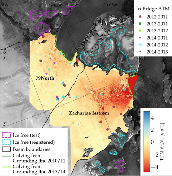
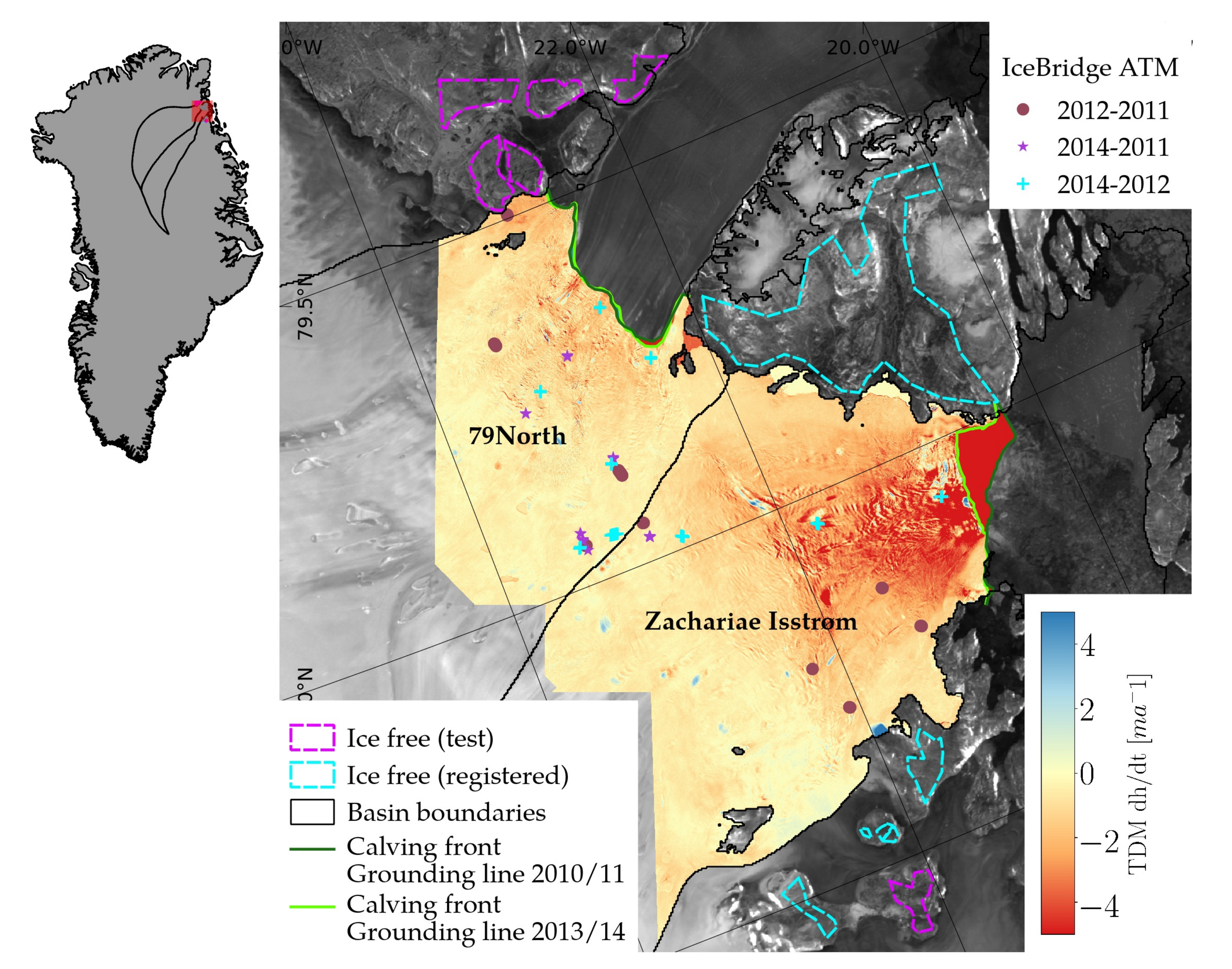
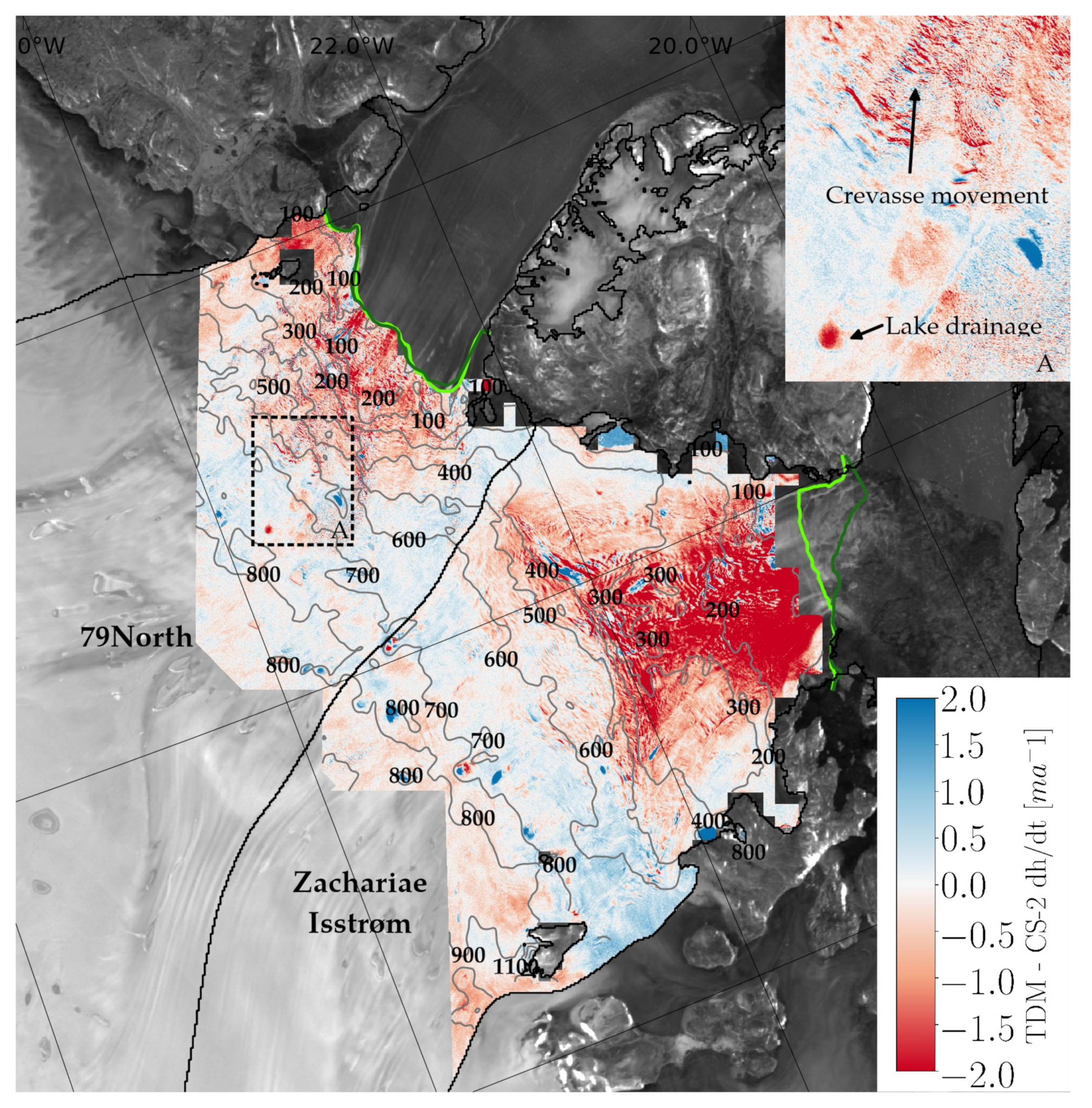
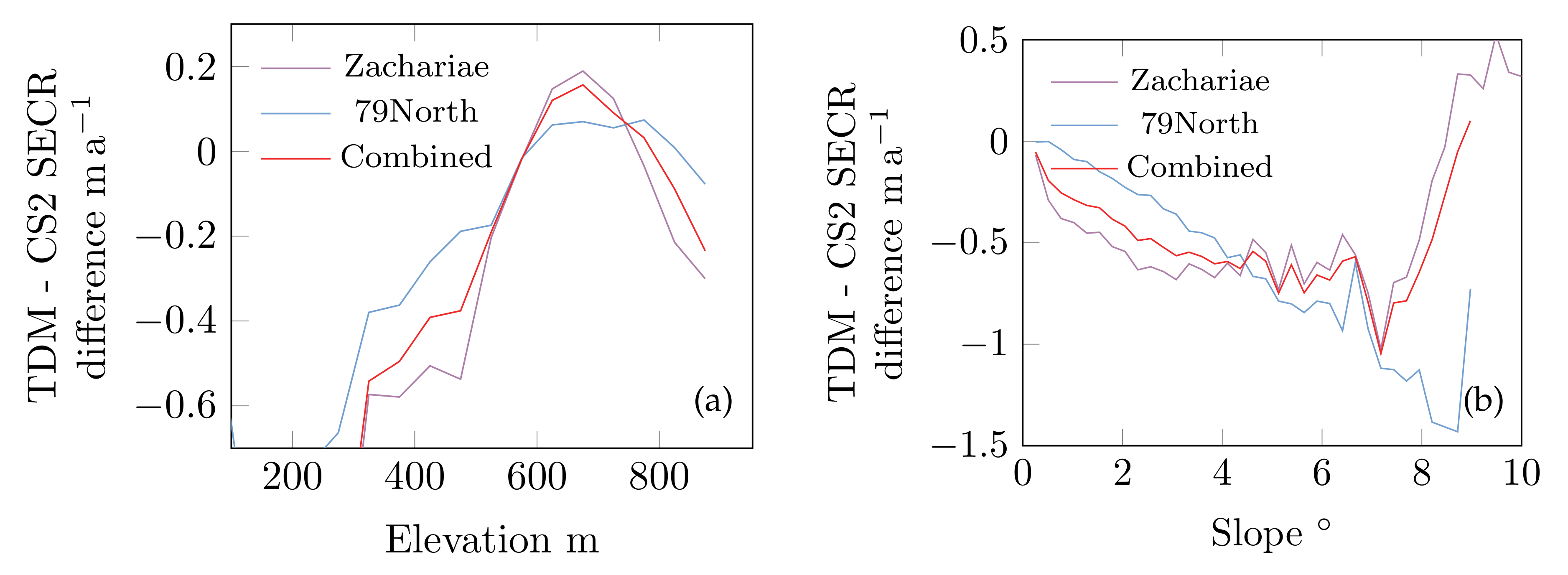
• The vertical bias between two differenced RawDEMs has been removed during vertical co-registration of all TDM RawDEMs. To estimate the uncertainty of this correction, we further analysed the SECR over flat, ice free areas that were not used during vertical co-registration (magenta areas in Figure 1) where no elevation change is expected. We measured remaining biases between $-0.04$ $\mathrm{m}$${\mathrm{a}}^{-1}$ and $0.13$ $\mathrm{m}$${\mathrm{a}}^{-1}$. Combined with the resulting differences to the CS-2 SECR in overlapping regions above 600 $\mathrm{m}$ shown in Figure 5a, we assumed a value of $0.2$ $\mathrm{m}$${\mathrm{a}}^{-1}$ as uncertainty in vertical co-registration for each pixel which is captured in the mass change uncertainty ${\sigma }_{m_{coreg}}$.
• Interferometric phase jumps and the resulting biases in the surface elevation change map can occur due to phase unwrapping errors during DEM generation. They appear as constant offsets in the DEM difference measurements. Areas possibly affected by phase unwrapping errors, radar shadow and layover are provided in a layer by ITP [30]. The resulting DEMs have been checked for such cases and no occurrences have been found in the observed area.
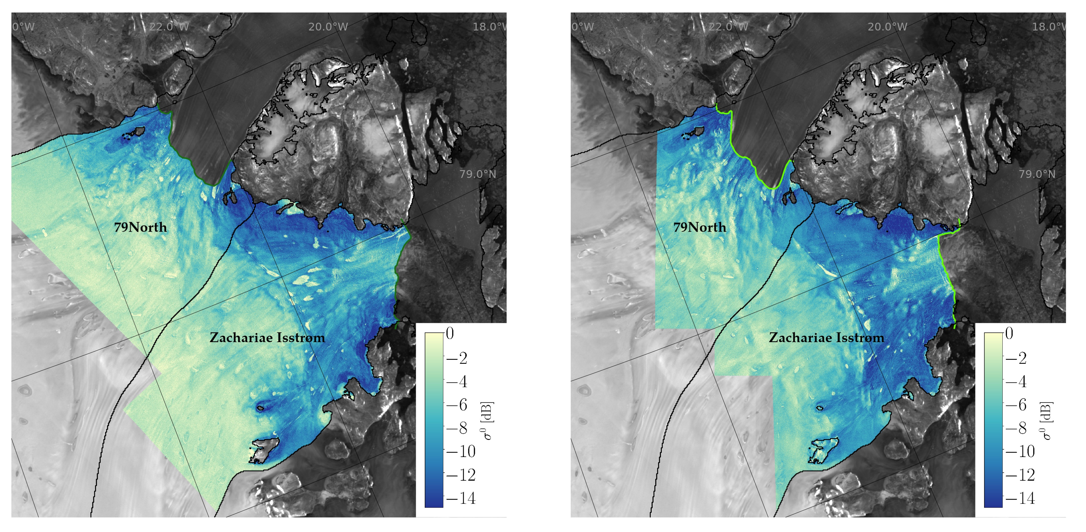
• Errors stemming from signal penetration into ice and snow could not be measured directly but are discussed in detail below. Because only the differences in signal penetration affect the measured SEC we assumed no uncertainties for areas with ${\sigma }^0>-3$ dB in both backscattering mosaics or where the absolute difference between the ${\sigma }^0$ values is <1 dB. In all other areas, the uncertainty due to signal penetration was set to $0.1$ $\mathrm{m}$${\mathrm{a}}^{-1}$. Note that elevation biases due to a difference in signal penetration would manifest themselves in Figure 5a. Therefore, part of this error has already been accounted for in the error budget of the vertical co-registration and larger biases due to signal penetration have been ruled out in this comparison. The mass change error due to signal penetration is termed ${\sigma }_{m_{pen}}$.

Finally, we form the combined mass balance uncertainty resulting from the TDM elevation change measurements.

$${\sigma }_{m_{TDM}}^2={\sigma }_{m_{ran}}^2+{\sigma }_{m_{pen}}^2+{\sigma }_{m_{coreg}}^2$$

(8)

Concerning the sub-aqueous mass loss uncertainty, the errors of the bedrock elevations in Morlighem et al. [33] were applied. The calving fronts were delineated by hand on the SAR amplitude images. Their spatial uncertainties are therefore small and were neglected.

In contrast to the altimeter elevation measurements, we used the InSAR DEMs as relative measurements without an absolute reference point. Their vertical co-registration is an important step and can introduce systematic biases in the SEC measurements. That is why we analysed the resulting SEC on stable ground and to CS-2 over glaciated, flat terrain (Figure 5). As discussed in [28], the TDM global DEM elevations which we used as a reference DEM are in turn co-registered to ICESat points but it is of benefit to use a reference DEM of high spatial resolution to increase the area over which vertical offsets of the RawDEMs can be measured. Because the SEC is a relative measurement, the exact choice and absolute accuracy of the chosen reference DEM is less critical and other high resolution DEMs such as the Arctic DEM [52] or GIMP [40] can be considered. An important criterion is, however, that there are no vertical offsets or inaccuracies within and between the calibration regions which are used for the vertical co-registration of the TDM RawDEMs. The used reference DEM was checked carefully in these regions and we also investigated vertical offsets in overlapping parts of the different TDM RawDEMs of the same year to avoid remaining biases in the resulting SEC.

Another addressed uncertainty in the DEM differencing based on InSAR measurements is the SAR signal penetration into ice and snow. It is dependent on the dielectric properties of ice and snow as well as the used wavelength [53]. Even a small liquid water content leads to a strong absorption of the signal which in turn causes a reduction of the penetration depth. In our case, the TDM acquisitions are in winter where a wet surface is ruled out and signal penetration has to be considered. Apart from the liquid water content, the structural properties of the snowpack or the ice surface affect the amount of penetration [54]. For the used X-band with a wavelength of 31 $\mathrm{m}$$\mathrm{m}$, the surface roughness in areas of fast flow near the crevassed terminus results in dominant surface scattering with high ${\sigma }^0$ values. Here, we did not account for a possible bias due to SAR signal penetration for backscattering values > 3 db. Furthermore, the entire observed area by TDM is located in the ablation zone and total, modelled SMB precipitation values are < 150 $\mathrm{m}$$\mathrm{m}$ water equivalent between end of ablation and the month of the acquisitions (September 2010–January 2011 and September 2013–January 2014). This is likely leading to a thin layer of relatively dry snow on the ice surface. A SAR tomography study with X- C- and L-band over the percolation zone [55] confirmed that the fresh and dry snow layer is generally transparent to the radar and that the scattering takes place at the previous summer layers. We therefore assume that a difference in the already small precipitation in the form of snowfall does not affect the captured surface elevation changes.

While the effect of SAR signal penetration can lead to an elevation bias of > 8 m for the dry snow zone on the GrIS [56], the bias in the actual difference of two X-band DEMs is much smaller when similar structural properties of the volume below the surface are present [22]. Therefore, no signal penetration uncertainty has been assumed for backscattering values that are sufficiently similar (within 1 ) in both mosaics. The map of ${\sigma }^0$ differences between the master and slave TDM acquisitions is shown in Figure S5 in the Supplementary Materials (Section S4). The maximal difference in incidence angles of 3${}^{\circ }$ between the master and slave acquisitions could also result in different penetration biases in the DEMs. It has a linear relationship to the penetration lengths and would result in a difference of approximately 6 $\mathrm{c}$$\mathrm{m}$ for penetration lengths of 2 $\mathrm{m}$. As strong scattering at the layers of previous summer surfaces can be expected in the ablation zone, the actual penetration is likely below 2 $\mathrm{m}$ and we have not considered the effect of a difference in incidence angles separately. For the same reason, no separate errors are calculated for possible biases resulting from the different ascending and descending headings. Instead, we included an error of $0.1$ $\mathrm{m}$${\mathrm{a}}^{-1}$ based on the ${\sigma }^0$ values, to account for a difference in elevation bias due to signal penetration which represents a 30 $\mathrm{c}$$\mathrm{m}$ difference in penetration bias in the master and slave DEMs.

3.2. Uncertainty of CS-2 Mass Change Rate

The CS-2 SECR height change estimates are provided with an individual uncertainty estimate for each grid cell. These are derived by the two processing steps, RAA and HFK.

The RAA a posteriori standard uncertainty is based on the statistics of the residuals (Equation (2)). These uncertainties are taken into account during the HFK interpolation process [47]. The final standard uncertainties are the square root of the HFK kriging variance ${\sigma }_{CS-2}$. The suitability of this uncertainty estimate was shown by Ströenreuther et al. [57] and the resulting map of 1$-\sigma$ uncertainties is provided in the Supplementary Materials (Section S5).

To calculate the mass balance uncertainty for CS-2 at the basin scale, we took spatial auto-correlation into account by following the approach of Rignot et al. [58]. We estimated empirical variograms using an exponential model fit with nugget n sill s, lag distance h and range a. Note that these are different parameters than the ones used in the sample variogram estimation during HFK (Section 2.2).

$$\gamma \left(h\right)=n+s(1-e^{\frac{-3h}{a}})$$

(9)

Correlation lengths of 500 $\mathrm{k}$$\mathrm{m}$ for elevations above 2000 $\mathrm{m}$ and below 140 $\mathrm{k}$$\mathrm{m}$ have been found. Both the errors of the CS-2 SECR and the uncertainties of the firn compaction rates were assumed to be correlated over these distances and were propagated together with the uncertainties in firn densities for the entire basins. To calculate ${\sigma }_{m_{CS-2}}$ and ${\sigma }_{m_{FC}}$, the correlation distances were used as in Equation (7) to integrate the pixel-wise mass balance uncertainties over the whole basin.

As mentioned in Section 2.2, the measurements of CS-2 (operating in Ku Band with $13.5$ GHz [38]) are affected by signal penetration. Contrary to the InSAR measurements no constant scattering properties can be assumed, and the different penetration biases have to be considered. Changes in penetration depth and snow structure impact the reflection layer. Especially with the melt event in 2012 refreezing melt layers lead to significant seasonal elevation differences. In addition, the scattering properties of the surface impact the waveform of the altimeter signal, including LeW and Bs [43]. Thus, Simonsen and Sørensen [44] showed that the penetration effect can be reduced by introducing different waveform parameter changes to RAA. Considering these changing signal parameters in RAA and using a low threshold retracker [20,59,60] reduce the effect of penetration in our CS-2 height change estimate.

4. Comparison to IceBridge ATM Elevation Changes

To validate the two SECR maps produced from TanDEM-X and CS-2, the measurements were compared to IceBridge ATM L4 Surface Elevation Rate of Change [61]. In the observation period between 2011 and 2014, there were several Operation IceBridge campaigns over the two basins with repeated measurements at crossover points or along the same flight line. In Figure 1 and Figure 3, the IceBridge laser altimeter ATM $\frac{dh}{dt}$ measurement locations and their respective time periods are visualised. For the comparison in

Table 2. $\frac{dh}{dt}$ comparison to IceBridge ATM (TDM/CS-2—ATM) for different time periods between 2011 and 2014. Differences have been extracted in patches of $500 \mathrm{m} \mathrm{x} 500$$\mathrm{m}$ for TDM and $750 \mathrm{m} \mathrm{x} 750$$\mathrm{m}$ for CS-2. The number of measurements # is the number of patches at which comparisons have been performed and relates to the sampling in the IceBridge ATM L4 products.

Sensor	Test Year	Ref. Year	${\mathit{\mu }}_{\frac{\mathit{dh}}{\mathit{dt}}}$ [$\mathbf{m}{\mathbf{a}}^{-1}$]	${\mathit{\sigma }}_{\frac{\mathit{dh}}{\mathit{dt}}}$ [$\mathbf{m}{\mathbf{a}}^{-1}$]	$\frac{\mathit{dh}}{\mathit{dt}}$ Median [$\mathbf{m}{\mathbf{a}}^{-1}$]	#
TDM	2012	2011	-0.213803	0.240390	-0.173089	70
	2014	2011	0.093840	0.210953	0.164076	63
	2014	2012	-0.456726	1.123732	-0.187544	104
	-	-	-0.238624	0.793954	-0.098592	237
CS-2	2012	2011	0.029139	0.115690	0.056126	392
	2013	2011	0.069246	0.070397	0.067729	6504
	2013	2012	0.219659	0.119956	0.183430	62
	2014	2011	0.031706	0.065367	0.038373	443
	2014	2012	0.090216	0.057170	0.085921	3920
	2014	2013	-0.055979	0.106620	-0.041550	11,814
	-	-	0.007857	0.111920	0.028002	23,135

, the difference between the IceBridge ATM measurements and our respective SECR was analysed (TDM/CS-2—ATM). For each given IceBridge ATM L4 measurement, the $\frac{dh}{dt}$ difference was extracted in patches of $500 \mathrm{m}\mathrm{\times }500$ $\mathrm{m}$ for TDM and $750 \mathrm{m}\mathrm{\times }750$ $\mathrm{m}$ for CS-2. In contrast to the TDM and CS-2 surface elevation changes, the IceBridge ATM laser-based measurements are not affected by signal penetration and were therefore used for comparison.

The mean difference for all IceBridge ATM measurements to the ones processed from CS-2 data is below $0.01$ $\mathrm{m}$${\mathrm{a}}^{-1}$ with greater variation for the individual time periods. Between 2012 and 2013, only 62 measurements at three locations were available and thus the larger mean difference of $0.22$ $\mathrm{m}$${\mathrm{a}}^{-1}$ compared to the other time periods can be explained. For the same reason, the differences to the TDM SECR are difficult to interpret. Overall, only 237 crossover locations were available where a median difference of $-0.10$ $\mathrm{m}$${\mathrm{a}}^{-1}$ was measured. However, the dataset is characterised by a large standard deviation of $0.79$ $\mathrm{m}$${\mathrm{a}}^{-1}$ and especially for the 2014–2012 time period, mean offsets of $-0.46$ $\mathrm{m}$${\mathrm{a}}^{-1}$ are large and exceed the combined uncertainties of signal penetration and inaccurate vertical co-registration of $0.30$ $\mathrm{m}$${\mathrm{a}}^{-1}$.

5. Results and Discussion

We report the final mass balance for both basins in

Table 3. $\frac{dM}{dt}$ estimates from the TDM/CS-2 combination for Zachariæ Isstrøm and 79North in the time period between 01/01/2011 and 31/12/2013 with and without contributions of the modelled firn compaction rate from the IMAU-FDM model [51]. The CS-2 (total) mass change was calculated for the entire basin while CS-2 (contrib.) only states the mass change for the area that contributes to the combined estimate (TDM+CS-2). The total mass loss is calculated excluding sub-aqueous mass change. The ice discharge D is calculated from the difference between the volumetric mass balance and modelled SMB (RACMO2) [62]. Units are $\mathrm{G}$$\mathrm{t}$${\mathrm{a}}^{-1}$.

Glacier Name	TDM $\frac{\mathit{dM}}{\mathit{dt}}$	CS-2 (contrib.) $\frac{\mathit{dM}}{\mathit{dt}}$	TDM+CS-2 $\frac{\mathit{dM}}{\mathit{dt}}$	CS-2 (total) $\frac{\mathit{dM}}{\mathit{dt}}$	Subaqua. $\frac{\mathit{dM}}{\mathit{dt}}$	SMB	D
Including firn compaction:
ZI	-5.37 ± 0.62	1.78 ± 0.96	-3.59 ± 1.15	-1.25± 1.00	-11.15 ± 0.03	8.95	−12.54
79North	-1.31 ± 0.34	0.30 ± 0.88	-1.01 ± 0.95	-0.62 ± 0.91	-0.05 ± 0.01	9.79	−10.80
Combined	-6.67 ± 0.71	2.08 ± 1.31	-4.60 ± 1.49	-1.87 ± 1.35	-11.20 ± 0.03	18.74	−23.34
No correction for firn compaction:
ZI	-5.37 ± 0.62	1.11 ± 0.96	-4.27 ± 1.14	-1.92 ± 0.99	-11.15 ± 0.03	8.95	−13.21
79North	-1.31 ± 0.34	-0.39 ± 0.88	-1.70 ± 0.94	-1.32 ± 0.90	-0.05 ± 0.01	9.79	−11.50
Combined	-6.68 ± 0.71	0.71 ± 1.30	-5.97 ± 1.48	-3.24 ± 1.34	-11.20 ± 0.03	18.74	−24.71

. Both glaciers display a negative mass balance. ZI has lost more than three times as much mass as its neighbouring glacier 79North. In this combination, 2.6% (ZI: 3.8%, 79North: 1.6%) of the basin was observed by TDM and the remaining 97.4% (ZI: 96.2%, 79North: 98.4%) by CS-2 resulting in an overall mass loss of $4.6\pm 1.49$ $\mathrm{G}$$\mathrm{t}$${\mathrm{a}}^{-1}$. If only CS-2 measurements were to be used for the entire basin without considering TDM data, the mass loss of NEGIS is only $1.87\pm 1.35$ $\mathrm{G}$$\mathrm{t}$${\mathrm{a}}^{-1}$. This difference highlights the difficulties of capturing the fast changing parts of the glacier termini accurately with conventional SARIn processing which underestimates mass loss by $2.73$ $\mathrm{G}$$\mathrm{t}$${\mathrm{a}}^{-1}$ in this case. We investigated the results of other CS-2 processing strategies in more detail, as presented in Section 5.2.

Close to the glacier terminus, the glaciers are subject to similar atmospheric forcing and the small differences in SMB [62] cannot explain the high differences in SEC alone. Ice dynamics are therefore identified as the main driver of the pronounced thinning on ZI. It shows surface lowering of up to 10 $\mathrm{m}$ ${\mathrm{a}}^{-1}$ compared to approximately 3 $\mathrm{m}$ ${\mathrm{a}}^{-1}$ at 79North. Mean surface lowering and volume change rates are provided in

Table 4. Mean TDM $\frac{dh}{dt}$ measurements and volume change rates $\frac{dV}{dt}$ for Zachariæ Isstrøm and 79North in the time period between 01/01/2011 and 31/12/2013. Sub-aqueous volume changes are not considered in this table. A is the area observed by TDM and represents only a fraction $A_{frac}$ of the entire catchments.

Glacier Name	A [$\mathbf{k}{\mathbf{m}}^2$]	${\mathit{A}}_{\mathbf{frac}}$ [%]	$\mathit{\mu }\frac{\mathit{dh}}{\mathit{dt}}$ [$\mathbf{m}{\mathbf{a}}^{-1}$]	$\frac{\mathit{dV}}{\mathit{dt}}$ [${\mathbf{k}}^3\mathbf{m}{\mathbf{a}}^{-1}$]	$\frac{\mathit{dM}}{\mathit{dt}}$ [$\mathbf{G}\mathbf{t}{\mathbf{a}}^{-1}$]
ZI	3221	3.8	-1.82 ± 0.55	-5.86 ± 0.67	-5.37 ± 0.62
79North	1784	1.6	-0.80 ± 0.55	-1.43 ± 0.37	-1.31 ± 0.34
Combined	5005	2.6	-2.62 ± 0.77	-7.29 ± 0.77	-6.67 ± 0.71

for areas observed by TDM.

While ZI’s floating ice tongue has steadily disintegrated from 2002 to 2014 [18], 79North’s ice tongue is thinning but still intact [63]. The loss of a buttressing ice tongue or ice shelf has been previously associated to subsequent speed-up and increased dynamic thinning [64]. Moreover, ZI has been rapidly retreating into the over 500 $\mathrm{m}$ deep fjord by an average of $2.1$ $\mathrm{k}$$\mathrm{m}$ during the observed time period. Using bedrock elevations from a combination of ice-penetrating radar measurements and a mass conservation approach [33], we calculated a substantial sub-aqueous mass loss of over 11 $\mathrm{G}$$\mathrm{t}$${\mathrm{a}}^{-1}$ assuming the glacier was grounded at both dates at the delineated calving front locations. Although this mass change does not have a direct impact on global sea level change, it still represents an important mass loss component that cannot be measured without calving front time series on high to medium resolution imagery. In the case of ZI, the sub-aqueous ice mass loss is about three times larger than the total glacier mass loss. The floating ice tongue of 79North has been excluded from the analysis, because of the tidal influence on surface elevation changes. Based on a combination of seismic bed profiles, optical data and TanDEM-X DEMs, 79North’s ice shelf has been shown to be losing mass through subglacial melting [63].

Although there is considerable melting in the ablation zone with a modelled surface mass balance from RACMO2.3p2 [62] of $-5.6$ $\mathrm{G}$$\mathrm{t}$${\mathrm{a}}^{-1}$ over both glaciers, the large accumulation zones (ZI: 81638 $\mathrm{k}$$\mathrm{m}$${}^2$ (95%), 79North: 103068 $\mathrm{k}$$\mathrm{m}$${}^2$ (94%)) currently counteract these losses. The overall mass loss of both outlet glaciers is therefore driven by dynamic ice export. To calculate ice discharge, the glacier surface mass balance was taken from the upsampled 1 $\mathrm{k}$$\mathrm{m}$ grid of RACMO2.3p2 [62] and subtracted from the total mass balance. The contribution of firn compaction over the combined basin of ZI and 79North equals 24% of the mass loss which is caused by measured $\frac{dh}{dt}$ alone. In contrast, GIA only accounts for 3% of this mass loss.

Our error bounds reported in Table 3 are relatively large, ranging between $0.34$ $\mathrm{G}$$\mathrm{t}$ $\mathrm{a}$ and $0.96$ $\mathrm{G}$$\mathrm{t}$ ${\mathrm{a}}^{-1}$. In the case of the TDM measurements, these are mainly attributed to the conservative systematic error budget for the vertical co-registration and signal penetration. For the CS-2 dataset, the errors are large mostly because of the large spatial correlation distances over 500 $\mathrm{k}$$\mathrm{m}$ and 140 $\mathrm{k}$$\mathrm{m}$ (see Section 3.2). The reported error budgets are approximately 1 $\mathrm{G}$$\mathrm{t}$ smaller in comparison to the volumetric mass balance estimates by Hurkmans et al. [10] and similar to the uncertainties for the mass-budget method employed by Mouginot and Rignot [19].

5.1. Comparison with Previous Mass Balance Estimates

Comparing our mass change values to previous studies, Hurkmans et al. [10] reported values for ZI of $0.1\pm 2.0$ $\mathrm{G}$$\mathrm{t}$${\mathrm{a}}^{-1}$ for 1996-2001 and $-1.3\pm 2.3$ $\mathrm{G}$$\mathrm{t}$ ${\mathrm{a}}^{-1}$ for 2003–2008 that are derived from volumetric changes measured by ERS-1 and ICESat. For the same time periods, 79North’s mass balance was estimated to be $0.4\pm 1.8$ $\mathrm{G}$$\mathrm{t}$${\mathrm{a}}^{-1}$ and $-0.9\pm 2.2$ $\mathrm{G}$$\mathrm{t}$ ${\mathrm{a}}^{-1}$, respectively. These epochs are 7 and 14 years prior to our study. Our values show increasing mass loss at ZI and a slower development for 79North which is partly balanced by larger mass gains in the accumulation zone. Another volumetric mass balance study in the same time period as ours has been published by McMillan et al. [12] stating a total mass loss of 8 $\mathrm{G}$$\mathrm{t}$ ($2.7$ $\mathrm{G}$$\mathrm{t}$ ${\mathrm{a}}^{-1}$) restricted to the ZI terminus region. Mass balance was calculated for the entirety of Greenland but has not been partitioned to the individual glacier level for all glaciers. Finally, Mouginot et al. [14] provided yearly estimates for individual glacier mass balances derived with the mass-budget method. Even though both glaciers have accelerated, the evolution of the mass balance for 79North is driven by year-to-year variations in SMB as ice discharge is only slightly increasing by approximately 1 $\mathrm{G}$$\mathrm{t}$ ${\mathrm{a}}^{-1}$ from 1995–2014 [14].

We show the comparisons of the different mass balance estimates in Figure 6. While results for ZI agree well, the volumetric mass losses reported here are more than 2 $\mathrm{G}$$\mathrm{t}$ ${\mathrm{a}}^{-1}$ smaller than the average mass loss measured with the mass-budget method at 79North during the three years. The reason for the discrepancy on 79North together with a good agreement at ZI is difficult to determine but can be caused by inaccuracies in the SMB model, the ice thickness or ice velocity measurements in case of the mass-budget method whereas the geodetic method is influenced by the FDM model, the ice density assumptions, and the SEC measurements. As the CS-2 SECR shows less than 1 $\mathrm{c}$$\mathrm{m}$ ${\mathrm{a}}^{-1}$ difference to the validation IceBridge ATM points (Table 2), possible error sources for the ice sheet interior are more likely for the density model or the firn compaction rates which dominate the volume change. For the region closer to the terminus an erroneous vertical co-registration of TDM is unlikely because of the good agreement on ZI which is comprised of the same RawDEM combination. A possible uncertainty in the vertical co-registration is accounted for in our mass balance uncertainty but it cannot explain the difference of 2 $\mathrm{G}$$\mathrm{t}$ ${\mathrm{a}}^{-1}$. Nevertheless, biases in the SEC due to a difference in penetration cannot be ruled out and may be different for the two glaciers. Because of the discrepancies in the mass balance measurements on 79North, different CS-2 $\frac{dh}{dt}$ measurements were analysed with our methodology, as presented below.

5.2. Comparison of Different CS-2 Processing Strategies

We calculated the mass loss for the ZI and 79North with different CS-2 processing strategies. Thus, we exchanged the CS-2 SECR maps for $\frac{dh}{dt}$ applying the processing of Helm et al. [20] and the methodology developed in Section 2.3 and Section 2.4. These SECR maps are based on the same measurements from the CS-2 Level-1B (Baseline C) data archive between 2011 and 2014. Similar preprocessing as for the CS-2 SECR map from TU Dresden was performed but different outlier elimination strategies were applied. Four versions of CS-2 SECR maps are available, which are detailed in

Table 5. The analysed CS-2 processing strategies with 10% OCOG [37] and TFMRA [20] retracker combinations for LRM and SARIn mode. The inclusion of the LeW and $bs$ parameters in the regression is detailed in Equation (2).

	LRM Retracking	SARIn Retracking	LeW in LRM Regression	$\mathbf{bs}$ in SARIn Regression
TU Dresden	10% OCOG	TFMRA	✓	✓
AWI swath	TFMRA	swath	-	-
AWI TFMRA	TFMRA	TFMRA	-	-
AWI TFMRA + LeW	TFMRA	TFMRA	✓	-

.

The AWI $\frac{dh}{dt}$ maps are generated following Helm et al. [20] with the multi-parameter regression being reduced to a linear fit of $\frac{dh}{dt}$ only. Topography within pixels of 2 $\mathrm{k}$$\mathrm{m}$ was accounted for by using the Arctic DEM [52] instead of fitting a two-dimensional surface. For the AWI $\frac{dh}{dt}$ TFMRA product, neither backscatter nor leading edge parameter, or a periodic parameter, has been applied within the regression. The reason is that we do not see a clear periodicity with a similar amplitude nor a high correlation with backscatter in the study area. However, the leading edge width (LeW) shows some correlation with LRM data, especially around July 2012 (which correlates with the surface melt event). Therefore, we provide the additional TFMRA + LeW product, where the LeW was used within the regression.

We calculated the mass balances for the different CS-2 input datasets with and without replacing the SECR rates in the terminus region by TDM data. The resulting measurements are reported in

Table 6. $\frac{dM}{dt}$ estimates for Zachariæ Isstrøm and 79North in the time period between 01/01/2011 and 31/12/2013 for different CS-2 processing strategies. Units are $\mathrm{G}$$\mathrm{t}$ ${\mathrm{a}}^{-1}$.

CS-2 Processing	TDM Processing	Zachariæ Isstrøm	79North	Total Mass Loss
TU Dresden	✓	-3.59 ± 1.15	-1.01 ± 0.95	-4.60 ± 1.49
TU Dresden	-	-1.25 ± 1.00	-0.62 ± 0.91	-1.87 ± 1.35
AWI swath	✓	-4.07 ± 3.86	-1.85 ± 3.48	-5.92 ± 5.19
AWI swath	-	-3.33 ± 3.88	-1.73 ± 3.53	-5.05 ± 5.24
AWI TFMRA	✓	-3.30 ± 1.53	-0.54 ± 1.29	-3.84 ± 2.00
AWI TFMRA	-	-1.15 ± 1.45	-0.18 ± 1.29	-1.33 ± 1.94
AWI TFMRA + LeW	✓	-3.95 ± 1.60	-1.05 ± 1.36	-5.00 ± 2.10
AWI TFMRA + LeW	-	-1.81 ± 1.53	-0.67 ± 1.35	-2.48 ± 2.04

and Figure 7. In all results which use solely CS-2 SECR, remaining data gaps at the glacier margin have been interpolated by a nearest neighbour interpolation and values over the retreating terminus (between the two calving fronts in Figure 1) were discarded. Instead, the TDM-derived mass balance due to terminus retreat of $-0.45$ $\mathrm{G}$$\mathrm{t}$ ${\mathrm{a}}^{-1}$ at ZI and $-0.01$ $\mathrm{G}$$\mathrm{t}$ ${\mathrm{a}}^{-1}$ at 79North was taken into account to make the dataset comparable.

Variations of volumetric mass balances among the four different CS-2 processing methodologies were found even without including the SECR from TDM. The discrepancies are mainly driven by the different processing of LRM data and how effective one can account for seasonal variability in radar backscattering. Especially the 2012 melt event led to a significant change of the dominant scattering mechanism for Ku-Band which strongly effected the estimated surface elevation of CryoSat-2 [43]. Simonsen and Sørensen [44] showed a correlation between LeW and elevation change and suggested to apply a LeW parameter within the regression for data products provided by ESA, which rely on OCOG (50% threshold) or model fits. Nilsson et al. [60] suggested a retracker (20% threshold) to account for this effect. Both the AWI TFMRA (25%) introduced by Helm et al. [20] and a 10% OCOG by TU Dresden are accounting for the majority of melt effect but a residual contribution might be present. Therefore, we also applied the LeW correlation within the regression for LRM data for the TU-Dresden and AWI TFMRA + LeW products.

When focusing on the SECR differences among the four different CS-2 datasets and the TDM $\frac{dh}{dt}$ map, we found that the CS-2 swath processing has the potential to improve CS-2 SECR over the fast changing parts of the glacier termini and shows smaller differences to TDM than conventional SARIn processing. However, the $\frac{dh}{dt}$ resulting from CS-2 swath processing is still underestimated compared to the TDM SECR. As a result, $0.87$ $\mathrm{G}$$\mathrm{t}$ ${\mathrm{a}}^{-1}$ more mass loss is measured over ZI and 79North, by including TDM SECR in a combined analysis with AWI swath $\frac{dh}{dt}$. A difference of spatially distributed SECR (TDM—CS-2) is presented in Figure 8. The respective comparisons over absolute elevation, slope and surface roughness for the AWI CS-2 swath processing can be found in the Supplementary Materials (Section S8).

The overall accuracy of our mass loss estimates is difficult to assess due to the unavailability of ground truth data for individual Greenland glaciers. Gravimetry is not applicable to the individual glacier scale, thus the mass-budget method represents the only other independent remote sensing technique delivering mass balance estimates for single glaciers. Because of the lack of ground truth mass change data, we focused on validating the SEC measurements instead. Our derived SECRs from both sensors (TDM, CS-2) were compared in a detailed analysis over slope, elevation and surface roughness (Section 2.3). Additionally, IceBridge ATM $\frac{dh}{dt}$ measurements were analysed for available crossover locations (Section 4). In the following, we discuss the range of possible mass balance estimates with different CS-2 processing strategies, which furthers the understanding of the accuracy of the synergistic method.

Especially for ZI, a good agreement of the synergistic mass loss values is reached and our values vary from 3.30$\mathrm{G}$$\mathrm{t}$ ${\mathrm{a}}^{-1}$–4.07$\mathrm{G}$$\mathrm{t}$ ${\mathrm{a}}^{-1}$ (Table 6). Whenever the TDM dataset was included, the derived mass loss increased for both glaciers (Figure 7). For the SARIn strategies, this gap to the synergistic mass balance (TDM included) varies from 2.14$\mathrm{G}$$\mathrm{t}$ ${\mathrm{a}}^{-1}$–2.34$\mathrm{G}$$\mathrm{t}$ ${\mathrm{a}}^{-1}$ at ZI and 0.33$\mathrm{G}$$\mathrm{t}$ ${\mathrm{a}}^{-1}$–0.38$\mathrm{G}$$\mathrm{t}$ ${\mathrm{a}}^{-1}$ at 79North. These constant offsets indicate that all SARIn strategies retrieve similar, but underestimated $\frac{dh}{dt}$ over the glacier termini. A special case is represented by CS-2 swath processing. Here, the inclusion of additional TDM data results only in $0.74$ $\mathrm{G}$$\mathrm{t}$ ${\mathrm{a}}^{-1}$ and $0.12$ $\mathrm{G}$$\mathrm{t}$ ${\mathrm{a}}^{-1}$ more mass loss at ZI and 79North, respectively. The differences between TDM and CS2-only processing are reduced in the CS-2 swath case compared to conventional SARIn processing. 79North shows surface lowering of up to 3 $\mathrm{m}$ ${\mathrm{a}}^{-1}$, and CS-2 swath is almost able to capture these changes to the same extent as TDM. However, the higher SECRs of up to 10 $\mathrm{m}$ ${\mathrm{a}}^{-1}$ are not recorded in the CS-2 swath data. This indicates an increasing importance of the synergistic TDM/CS-2 mass loss for glaciers with high SECR.

We were able to reduce the discrepancies of mass balance estimates between the mass-budget method and volumetric methods with the developed synergistic approach. All our estimates which include TDM measurements perform closer to the values of Mouginot et al. [14] than their CS-2-only counterparts (Figure 7). On 79North, however, none of the above-presented volumetric techniques can reproduce the budget-derived mass loss (including and excluding TDM). We therefore believe that the discharge at 79North is possibly overestimated. Complementary mass balance estimates from the geodetic method and the mass-budget method for the same time frame will provide the basis to investigate possible remaining error sources in either of the measurements.

6. Conclusions

This study presents a novel combination of CryoSat-2 and TanDEM-X elevation changes to be used in the context of calculating the geodetic mass balance of individual outlet glaciers on ice sheets. This makes it feasible for InSAR DEM differencing to contribute to volumetric mass balance estimates on major outlet glaciers in Greenland and eliminates the need to cover the entire glacier basin with timely bistatic InSAR acquisitions. Furthermore, the two sensors complement each other with their different horizontal resolutions as well as vertical accuracies making it a superior approach compared to using data from a single sensor only. Utilising the entire time series of elevation measurements together with the ability to retrack the radar waveform makes radar altimetry the better suited method to measure the smaller elevation changes in the firn and snow covered areas of the ice sheet interior and allows a gapless observation of 100% of the drainage basin. Complementary, single-pass interferometry is able to resolve the higher resolution spatial details on the glacier terminus with larger surface elevation changes where surface scattering dominates because of the rough ice surface. We show that conventional CS-2 SARIn processing underestimates mass loss in these areas. The range of mass balance results using different CS-2 processing strategies was investigated and the potential of CS-2 swath processing over the fast changing glacier termini was presented. We propose to repeat these synergistic mass balance measurements for other major outlet glaciers in Greenland or Antarctica complementary to budget-method derived mass balance observations for individual outlet glaciers. In the cases of ZI and 79North, we report geodetic mass balances of $-3.59\pm 1.15$ $\mathrm{G}$$\mathrm{t}$ ${\mathrm{a}}^{-1}$ and $-1.01\pm 0.95$ $\mathrm{G}$$\mathrm{t}$ ${\mathrm{a}}^{-1}$, respectively. According to these values, the two glaciers are losing less mass than previously reported with the mass-budget method [14]. The discrepancies between the two methods require further investigation.

References

1. Vaughan, D.G.; Comiso, J.C.; Allison, I.; Carrasco, J.; Kaser, G.; Kwok, R.; Mote, P.; Murray, T.; Paul, F.; Ren, J.; et al. Observations: Cryosphere. Clim. Chang. 2013, 2103, 317–382. [Google Scholar]
2. Van den Broeke, M.R.; Bamber, J.L.; Ettema, J.; Rignot, E.; Schrama, E.J.O.; van de Berg, W.J.; van Meijgaard, E.; Velicogna, I.; Wouters, B. Partitioning Recent Greenland Mass Loss. Science 2009, 326, 984–986. [Google Scholar] [CrossRef] [PubMed] [Green Version]
3. Hanna, E.; Navarro, F.J.; Pattyn, F.; Domingues, C.M.; Fettweis, X.; Ivins, E.R.; Nicholls, R.J.; Ritz, C.; Smith, B.; Tulaczyk, S.; et al. Ice-Sheet Mass Balance and Climate Change. Nature 2013, 498, 51–59. [Google Scholar] [CrossRef] [PubMed]
4. Shepherd, A.; Ivins, E.R.; Geruo, A.; Barletta, V.R.; Bentley, M.J.; Bettadpur, S.; Briggs, K.H.; Bromwich, D.H.; Forsberg, R.; Galin, N.; et al. A Reconciled Estimate of Ice-Sheet Mass Balance. Science 2012, 338, 1183–1189. [Google Scholar] [CrossRef] [PubMed] [Green Version]
5. Khan, S.A.; Aschwanden, A.; Bjørk, A.A.; Wahr, J.; Kjeldsen, K.K.; Kjær, K.H. Greenland Ice Sheet Mass Balance: A Review. Rep. Prog. Phys. 2015, 78, 046801. [Google Scholar] [CrossRef] [PubMed]
6. Moon, T.; Joughin, I.R.; Smith, B.; Howat, I.M. 21st-Century Evolution of Greenland Outlet Glacier Velocities. Science 2012, 336, 576–578. [Google Scholar] [CrossRef] [Green Version]
7. Kehrl, L.M.; Joughin, I.R.; Shean, D.E.; Floricioiu, D.; Krieger, L. Seasonal and Interannual Variabilities in Terminus Position, Glacier Velocity, and Surface Elevation at Helheim and Kangerlussuaq Glaciers from 2008 to 2016. J. Geophys. Res. Earth Surf. 2017, 122, 1635–1652. [Google Scholar] [CrossRef]
8. Khan, S.A.; Kjær, K.H.; Bevis, M.; Bamber, J.L.; Wahr, J.; Kjeldsen, K.K.; Bjørk, A.A.; Korsgaard, N.J.; Stearns, L.A.; van den Broeke, M.R.; et al. Sustained Mass Loss of the Northeast Greenland Ice Sheet Triggered by Regional Warming. Nat. Clim. Chang. 2014, 4, 292–299. [Google Scholar] [CrossRef]
9. Krieger, L.; Floricioiu, D.; Neckel, N. Drainage Basin Delineation for Outlet Glaciers of Northeast Greenland Based on Sentinel-1 Ice Velocities and TanDEM-X Elevations. Remote Sens. Environ. 2020, 237, 111483. [Google Scholar] [CrossRef]
10. Hurkmans, R.T.W.L.; Bamber, J.L.; Davis, C.H.; Joughin, I.R.; Khvorostovsky, K.S.; Smith, B.S.; Schoen, N. Time-Evolving Mass Loss of the Greenland Ice Sheet from Satellite Altimetry. Cryosphere 2014, 8, 1725–1740. [Google Scholar] [CrossRef] [Green Version]
11. McMillan, M.; Shepherd, A.; Sundal, A.V.; Briggs, K.H.; Muir, A.; Ridout, A.J.; Hogg, A.E.; Wingham, D.J. Increased Ice Losses from Antarctica Detected by CryoSat-2. Geophys. Res. Lett. 2014, 41, 3899–3905. [Google Scholar] [CrossRef]
12. McMillan, M.; Leeson, A.; Shepherd, A.; Briggs, K.H.; Armitage, T.W.K.; Hogg, A.E.; Munneke, P.K.; van den Broeke, M.R.; Noël, B.P.Y.; van de Berg, W.J.; et al. A High-Resolution Record of Greenland Mass Balance. Geophys. Res. Lett. 2016, 43, 7002–7010. [Google Scholar] [CrossRef] [Green Version]
13. Enderlin, E.M.; Howat, I.M.; Jeong, S.; Noh, M.J.; van Angelen, J.H.; van den Broeke, M.R. An Improved Mass Budget for the Greenland Ice Sheet. Geophys. Res. Lett. 2014, 41, 866–872. [Google Scholar] [CrossRef] [Green Version]
14. Mouginot, J.; Rignot, E.; Bjørk, A.A.; van den Broeke, M.R.; Millan, R.; Morlighem, M.; Noël, B.P.Y.; Scheuchl, B.; Wood, M. Forty-Six Years of Greenland Ice Sheet Mass Balance from 1972 to 2018. Proc. Natl. Acad. Sci. USA 2019, 116, 9239–9244. [Google Scholar] [CrossRef] [Green Version]
15. Luthcke, S.B.; Zwally, H.J.; Abdalati, W.; Rowlands, D.D.; Ray, R.D.; Nerem, R.S.; Lemoine, F.G.; McCarthy, J.J.; Chinn, D.S. Recent Greenland Ice Mass Loss by Drainage System from Satellite Gravity Observations. Science 2006, 314, 1286–1289. [Google Scholar] [CrossRef] [Green Version]
16. Sasgen, I.; van den Broeke, M.; Bamber, J.L.; Rignot, E.; Sørensen, L.S.; Wouters, B.; Martinec, Z.; Velicogna, I.; Simonsen, S.B. Timing and Origin of Recent Regional Ice-Mass Loss in Greenland. Earth Planet. Sci. Lett. 2012, 333-334, 293–303. [Google Scholar] [CrossRef] [Green Version]
17. Howat, I.M.; Ahn, Y.; Joughin, I.; van den Broeke, M.R.; Lenaerts, J.T.M.; Smith, B. Mass Balance of Greenland’s Three Largest Outlet Glaciers, 2000–2010. Geophys. Res. Lett. 2011, 38. [Google Scholar] [CrossRef] [Green Version]
18. Mouginot, J.; Rignot, E.; Scheuchl, B.; Fenty, I.; Khazendar, A.; Morlighem, M.; Buzzi, A.; Paden, J. Fast Retreat of Zachariæ Isstrøm, Northeast Greenland. Science 2015, 350, 1357–1361. [Google Scholar] [CrossRef] [Green Version]
19. Mouginot, J.; Rignot, E. Glacier Catchments/Basins for the Greenland Ice Sheet; UC Irvine Dash: Irvine, CA, USA, 2019. [Google Scholar] [CrossRef]
20. Helm, V.; Humbert, A.; Miller, H. Elevation and Elevation Change of Greenland and Antarctica Derived from CryoSat-2. Cryosphere 2014, 8, 1539–1559. [Google Scholar] [CrossRef] [Green Version]
21. Abdel Jaber, W.; Rott, H.; Floricioiu, D.; Wuite, J.; Miranda, N. Heterogeneous Spatial and Temporal Pattern of Surface Elevation Change and Mass Balance of the Patagonian Ice Fields between 2000 and 2016. Cryosphere 2019, 13, 2511–2535. [Google Scholar] [CrossRef] [Green Version]
22. Rott, H.; Abdel Jaber, W.; Wuite, J.; Scheiblauer, S.; Floricioiu, D.; van Wessem, J.M.; Nagler, T.; Miranda, N.; van den Broeke, M.R. Changing Pattern of Ice Flow and Mass Balance for Glaciers Discharging into the Larsen A and B Embayments, Antarctic Peninsula, 2011 to 2016. Cryosphere 2018, 12, 1273–1291. [Google Scholar] [CrossRef] [Green Version]
23. Braun, M.H.; Malz, P.; Sommer, C.; Farías-Barahona, D.; Sauter, T.; Casassa, G.; Soruco, A.; Skvarca, P.; Seehaus, T.C. Constraining Glacier Elevation and Mass Changes in South America. Nat. Clim. Chang. 2019, 9, 130–136. [Google Scholar] [CrossRef]
24. Dussaillant, I.; Berthier, E.; Brun, F.; Masiokas, M.; Hugonnet, R.; Favier, V.; Rabatel, A.; Pitte, P.; Ruiz, L. Two Decades of Glacier Mass Loss along the Andes. Nat. Geosci. 2019, 12, 802–808. [Google Scholar] [CrossRef]
25. Joughin, I.R.; Shean, D.E.; Smith, B.E.; Floricioiu, D. A Decade of Variability on Jakobshavn Isbrae: Ocean Temperatures Pace Speed Through Influence on Mélange Rigidity. Cryosphere Discuss. 2019, 1–27. [Google Scholar] [CrossRef] [Green Version]
26. Milillo, P.; Rignot, E.; Rizzoli, P.; Scheuchl, B.; Mouginot, J.; Bueso-Bello, J.; Prats-Iraola, P. Heterogeneous Retreat and Ice Melt of Thwaites Glacier, West Antarctica. Sci. Adv. 2019, 5, eaau3433. [Google Scholar] [CrossRef] [Green Version]
27. Krieger, G.; Moreira, A.; Fiedler, H.; Hajnsek, I.; Werner, M.; Younis, M.; Zink, M. TanDEM-X: A Satellite Formation for High-Resolution SAR Interferometry. IEEE Trans. Geosci. Remote Sens. 2007, 45, 3317–3341. [Google Scholar] [CrossRef] [Green Version]
28. Wessel, B.; Bertram, A.; Gruber, A.; Bemm, S.; Dech, S. A new high-resolution elevation model of Greenland derived from TanDEM-X. ISPRS Ann. Photogramm. Remote Sens. Spat. Inf. Sci. 2016, 7, 9–16. [Google Scholar] [CrossRef]
29. Wingham, D.J.; Rapley, C.G.; Griffiths, H. New Techniques in Satellite Altimeter Tracking Systems. In Proceedings of the 1986 International Geoscience and Remote Sensing Symposium (IGARSS’86) on Remote Sensing: Today’s Solutions for Tomorrow’s Information Needs; ESA SP-254:1339–1344; ESA: Zürich, Switzerland, 1986. [Google Scholar]
30. Rossi, C.; Eineder, M.; Fritz, T.; Breit, H. TanDEM-X Mission: Raw DEM Generation. In Proceedings of the 8th European Conference on Synthetic Aperture Radar, Aachen, Germany, 7–10 June 2010; pp. 1–4. [Google Scholar]
31. Rizzoli, P.; Martone, M.; Gonzalez, C.; Wecklich, C.; Borla Tridon, D.; Bräutigam, B.; Bachmann, M.; Schulze, D.; Fritz, T.; Huber, M.; et al. Generation and Performance Assessment of the Global TanDEM-X Digital Elevation Model. ISPRS J. Photogramm. Remote Sens. 2017, 132, 119–139. [Google Scholar] [CrossRef] [Green Version]
32. Breit, H.; Fritz, T.; Balss, U.; Lachaise, M.; Niedermeier, A.; Vonavka, M. TerraSAR-X SAR Processing and Products. IEEE Trans. Geosci. Remote Sens. 2010, 48, 727–740. [Google Scholar] [CrossRef]
33. Morlighem, M.; Williams, C.N.; Rignot, E.; An, L.; Arndt, J.E.; Bamber, J.L.; Catania, G.A.; Chauché, N.; Dowdeswell, J.A.; Dorschel, B.; et al. BedMachine v3: Complete Bed Topography and Ocean Bathymetry Mapping of Greenland From Multibeam Echo Sounding Combined with Mass Conservation. Geophys. Res. Lett. 2017, 44, 11051–11061. [Google Scholar] [CrossRef] [Green Version]
34. Legrésy, B.; Rémy, F.; Blarel, F. Along Track Repeat Altimetry for Ice Sheets and Continental Surface Studies. In Proceedings Symposium on 15 Years of Progress in Radar Altimetry; ESA-SP No. 614, Paper No. 181; European Space Agency Publication Division: Noordwijk, The Netherlands, 2006. [Google Scholar]
35. Flament, T.; Rémy, F. Dynamic Thinning of Antarctic Glaciers from Along-Track Repeat Radar Altimetry. J. Glaciol. 2012, 58, 830–840. [Google Scholar] [CrossRef] [Green Version]
36. Sørensen, L.S.; Simonsen, S.B.; Forsberg, R.; Khvorostovsky, K.; Meister, R.; Engdahl, M.E. 25 Years of Elevation Changes of the Greenland Ice Sheet from ERS, Envisat, and CryoSat-2 Radar Altimetry. Earth Planet. Sci. Lett. 2018, 495, 234–241. [Google Scholar] [CrossRef]
37. Schröder, L.; Horwath, M.; Dietrich, R.; Helm, V.; van den Broeke, M.R.; Ligtenberg, S.R.M. Four Decades of Antarctic Surface Elevation Changes from Multi-Mission Satellite Altimetry. Cryosphere 2019, 13, 427–449. [Google Scholar] [CrossRef] [Green Version]
38. Wingham, D.J.; Francis, C.R.; Baker, S.; Bouzinac, C.; Brockley, D.; Cullen, R.; de Chateau-Thierry, P.; Laxon, S.W.; Mallow, U.; Mavrocordatos, C.; et al. CryoSat: A Mission to Determine the Fluctuations in Earth’s Land and Marine Ice Fields. Adv. Space Res. 2006, 37, 841–871. [Google Scholar] [CrossRef]
39. Roemer, S.; Legrésy, B.; Horwath, M.; Dietrich, R. Refined Analysis of Radar Altimetry Data Applied to the Region of the Subglacial Lake Vostok/Antarctica. Remote Sens. Environ. 2007, 106, 269–284. [Google Scholar] [CrossRef]
40. Howat, I.M.; Negrete, A.; Smith, B.E. The Greenland Ice Mapping Project (GIMP) Land Classification and Surface Elevation Data Sets. Cryosphere 2014, 8, 1509–1518. [Google Scholar] [CrossRef] [Green Version]
41. Sørensen, L.S.; Simonsen, S.B.; Nielsen, K.; Lucas-Picher, P.; Spada, G.; Adalgeirsdottir, G.; Forsberg, R.; Hvidberg, C.S. Mass Balance of the Greenland Ice Sheet (2003–2008) from ICESat Data—The Impact of Interpolation, Sampling and Firn Density. Cryosphere 2011, 5, 173–186. [Google Scholar] [CrossRef] [Green Version]
42. Ewert, H.; Groh, A.; Dietrich, R. Volume and Mass Changes of the Greenland Ice Sheet Inferred from ICESat and GRACE. J. Geodyn. 2012, 59-60, 111–123. [Google Scholar] [CrossRef]
43. Nilsson, J.; Vallelonga, P.; Simonsen, S.B.; Sørensen, L.S.; Forsberg, R.; Dahl-Jensen, D.; Hirabayashi, M.; Goto-Azuma, K.; Hvidberg, C.S.; Kjær, H.A.; et al. Greenland 2012 Melt Event Effects on CryoSat-2 Radar Altimetry. Geophys. Res. Lett. 2015, 42, 3919–3926. [Google Scholar] [CrossRef]
44. Simonsen, S.B.; Sørensen, L.S. Implications of Changing Scattering Properties on Greenland Ice Sheet Volume Change from Cryosat-2 Altimetry. Remote Sens. Environ. 2017, 190, 207–216. [Google Scholar] [CrossRef]
45. Legrésy, B.; Rémy, F. Altimetric Observations of Surface Characteristics of the Antarctic Ice Sheet. J. Glaciol. 1997, 43, 265–275. [Google Scholar] [CrossRef] [Green Version]
46. Burgess, E.W.; Forster, R.R.; Box, J.E.; Mosley-Thompson, E.; Bromwich, D.H.; Bales, R.C.; Smith, L.C. A Spatially Calibrated Model of Annual Accumulation Rate on the Greenland Ice Sheet (1958–2007). J. Geophys. Res.: Earth Surf. 2010, 115. [Google Scholar] [CrossRef]
47. Christensen, W.F. Filtered Kriging for Spatial Data with Heterogeneous Measurement Error Variances. Biometrics 2011, 67, 947–957. [Google Scholar] [CrossRef] [PubMed]
48. Wake, L.M.; Lecavalier, B.S.; Bevis, M. Glacial Isostatic Adjustment (GIA) in Greenland: A Review. Curr. Clim. Chang. Rep. 2016, 2, 101–111. [Google Scholar] [CrossRef] [Green Version]
49. Peltier, W.R. Global Glacial Isostasy and the Surface of the Ice-Age Earth: The ice-5G (VM2) Model and GRACE. Annu. Rev. Earth Planet. Sci. 2004, 32, 111–149. [Google Scholar] [CrossRef]
50. Kuipers Munneke, P.; Ligtenberg, S.R.M.; Noël, B.P.Y.; Howat, I.M.; Box, J.E.; Mosley-Thompson, E.; McConnell, J.R.; Steffen, K.; Harper, J.T.; Das, S.B.; et al. Elevation Change of the Greenland Ice Sheet Due to Surface Mass Balance and Firn Processes, 1960–2014. Cryosphere 2015, 9, 2009–2025. [Google Scholar] [CrossRef] [Green Version]
51. Ligtenberg, S.R.M.; Kuipers Munneke, P.; Noël, B.P.Y.; van den Broeke, M.R. Brief Communication: Improved Simulation of the Present-Day Greenland Firn Layer (1960–2016). Cryosphere 2018, 12, 1643–1649. [Google Scholar]
52. Porter, C.; Morin, P.; Howat, I.; Noh, M.J.; Bates, B.; Peterman, K.; Keesey, S.; Schlenk, M.; Gardiner, J.; Tomko, K.; et al. ArcticDEM Harvard Dataverse V1; visited on 06/12/2019; Polar Geospatial Center: St. Paul, MN, USA, 2018. [Google Scholar] [CrossRef]
53. Mätzler, C. Applications of the Interaction of Microwaves with the Natural Snow Cover. Remote Sens. Rev. 1987, 2, 259–387. [Google Scholar] [CrossRef]
54. Stiles, W.; Ulaby, F. Dielectric Properties of Snow, RSL Technical Report 527-1, 1981. Available online: https://pdfs.semanticscholar.org/929e/a3c9076ec2b65defb9f5974f1b0180da41d5.pdf (accessed on 1 March 2020).
55. Fischer, G.; Jäger, M.; Papathanassiou, K.; Hajnsek, I. Modeling the Vertical Backscattering Distribution in the Percolation Zone of the Greenland Ice Sheet with SAR Tomography. IEEE J. Sel. Top. Appl. Earth Obs. Remote Sens. 2019, 12, 4389–4405. [Google Scholar] [CrossRef]
56. Rizzoli, P.; Martone, M.; Rott, H.; Moreira, A. Characterization of Snow Facies on the Greenland Ice Sheet Observed by TanDEM-X Interferometric SAR Data. Remote Sens. 2017, 9, 315. [Google Scholar] [CrossRef] [Green Version]
57. Strößenreuther, U.; Horwath, M.; Schröder, L. How Different Analysis and Interpolation Methods Affect the Accuracy of Ice Surface Elevation Changes Inferred from Satellite Altimetry. Math. Geosci. 2020. [Google Scholar] [CrossRef] [Green Version]
58. Rignot, E.; Bamber, J.L.; van den Broeke, M.R.; Davis, C.; Li, Y.; van de Berg, W.J.; van Meijgaard, E. Recent Antarctic Ice Mass Loss from Radar Interferometry and Regional Climate Modelling. Nat. Geosci. 2008, 1, 106–110. [Google Scholar] [CrossRef] [Green Version]
59. Davis, C. A Robust Threshold Retracking Algorithm for Measuring Ice-Sheet Surface Elevation Change from Satellite Radar Altimeters. IEEE Trans. Geosci. Remote Sens. 1997, 35, 974–979. [Google Scholar] [CrossRef]
60. Nilsson, J.; Gardner, A.; Sandberg Sørensen, L.; Forsberg, R. Improved Retrieval of Land Ice Topography from CryoSat-2 Data and Its Impact for Volume-Change Estimation of the Greenland Ice Sheet. Cryosphere 2016, 10, 2953–2969. [Google Scholar] [CrossRef] [Green Version]
61. Studinger, M. IceBridge ATM L4 Surface Elevation Rate of Change, Version 1; NASA National Snow and Ice Data Center Distributed Active Archive Center: Boulder, CO, USA, 2014; updated 2018. [Google Scholar]
62. Noël, B.P.Y.; van de Berg, W.J.; van Wessem, J.M.; van Meijgaard, E.; van As, D.; Lenaerts, J.T.M.; Lhermitte, S.; Kuipers Munneke, P.; Smeets, C.J.P.P.; van Ulft, L.H.; et al. Modelling the Climate and Surface Mass Balance of Polar Ice Sheets Using RACMO2—Part 1: Greenland (1958–2016). Cryosphere 2018, 12, 811–831. [Google Scholar] [CrossRef] [Green Version]
63. Mayer, C.; Schaffer, J.; Hattermann, T.; Floricioiu, D.; Krieger, L.; Dodd, P.A.; Kanzow, T.; Licciulli, C.; Schannwell, C. Large Ice Loss Variability at Nioghalvfjerdsfjorden Glacier, Northeast-Greenland. Nat. Commun. 2018, 9, 1–11. [Google Scholar] [CrossRef] [Green Version]
64. Rott, H.; Rack, W.; Skvarca, P.; Angelis, H.D. Northern Larsen Ice Shelf, Antarctica: Further Retreat after Collapse. Ann. Glaciol. 2002, 34, 277–282. [Google Scholar] [CrossRef] [Green Version]
Figure 1. Surface elevation change rates for Zachariæ Isstrøm and 79North measured by DEM differencing of TDM mosaics from winter 2010 and winter 2013. Ice free areas that have been used for vertical co-registration (blue) and uncertainty estimation (magenta) are superimposed on the TDM global DEM backscattering mosaic. Available locations of IceBridge ATM d h d t measurements are indicated for various sub-epochs. A detailed comparison to the IceBridge ATM data can be found in Section 4.
Remotesensing 12 00996 g001
Figure 2. σ 0 mosaics for winter 2010 and winter 2013 corrected for the noise equivalent σ 0 (NESZ). In the background, the TDM global DEM backscattering mosaic.
Remotesensing 12 00996 g002
Figure 3. Surface elevation change rates for Zachariæ Isstrøm and 79North measured by CS-2 RAA from January 2011 to January 2014 and superimposed footprints of IceBridge ATM overflights. A detailed comparison to the IceBridge ATM data can be found in Section 4. In the background is the TDM global DEM backscattering mosaic.
Remotesensing 12 00996 g003
Figure 4. Difference of the TDM SECR map and the CS-2 SECR (TDM—CS-2) for the termini of Zachariæ Isstrøm and 79North where measurements from both sensors overlap. Contour lines for absolute elevation are shown for the interpretation of Figure 5a. Calving fronts (green lines) and basin delineation (black line) are in Figure 1. Inset A shows differences in elevation change because of lake drainage and crevasse movement that is only captured in the high resolution TDM dataset.
Remotesensing 12 00996 g004
Figure 5. Differences of the TDM SECR map compared to the CS-2 SECR (TDM—CS-2) plotted over (a) elevation bins of 50 m and (b) surface slopes calculated from the TDM global DEM. The differences are calculated for the two basins separately and for all points combined.
Remotesensing 12 00996 g005
Figure 6. Comparison of mass balance results of the TDM/CS-2 combination with the volumetric approach of Hurkmans et al. [10] and the mass-budget method by Mouginot et al. [14] for individual glacier basins of (a) Zachariæ Isstrøm (ZI) and (b) Nioghalvfjerdsfjorden (79North).
Remotesensing 12 00996 g006
Figure 7. Mass loss from the volumetric approach of Hurkmans et al. [10] and the mass-budget method by Mouginot et al. [14] together with results from different combinations of surface elevation change measurements as in Table 6. The mass losses are partitioned to the individual glacier basins of (a) Zachariæ Isstrøm (ZI) and (b) Nioghalvfjerdsfjorden (79North). For better visibility, the mass losses are plotted without uncertainty bars.
Remotesensing 12 00996 g007
Figure 8. Differences of the TDM SECR map compared to the CS-2 surface elevation change trends from AWI swath processing (TDM—CS-2 AWI swath) for the terminus region of Zachariæ Isstrøm and 79North where SEC from both sensors is available.
Remotesensing 12 00996 g008