Figure 1.
Architecture of the Chronological Order Reverse Network (CORN).
Figure 1.
Architecture of the Chronological Order Reverse Network (CORN).
Figure 2.
Architecture of CORN with an additional skip connection to both decoder sides.
Figure 2.
Architecture of CORN with an additional skip connection to both decoder sides.
Figure 3.
Optical image showing an example of new constructions of Bangkok testing area. The size of each image is 1.3 × 1.3 km. (a) Time 1 image of first testing area from 22 August 2008, (b) Time 2 image of first testing area from 18 December 2009, (c) Time 1 image of second testing area from 10 February 2005, (d) Time 2 image of second testing area from 18 December 2009.
Figure 4.
Optical image showing an example of new constructions of Hanoi testing area. The size of each image is 2 × 2 km. (a) Time 1 image from 15 November 2002, (b) Time 2 image from 9 February 2010.
Figure 4.
Optical image showing an example of new constructions of Hanoi testing area. The size of each image is 2 × 2 km. (a) Time 1 image from 15 November 2002, (b) Time 2 image from 9 February 2010.
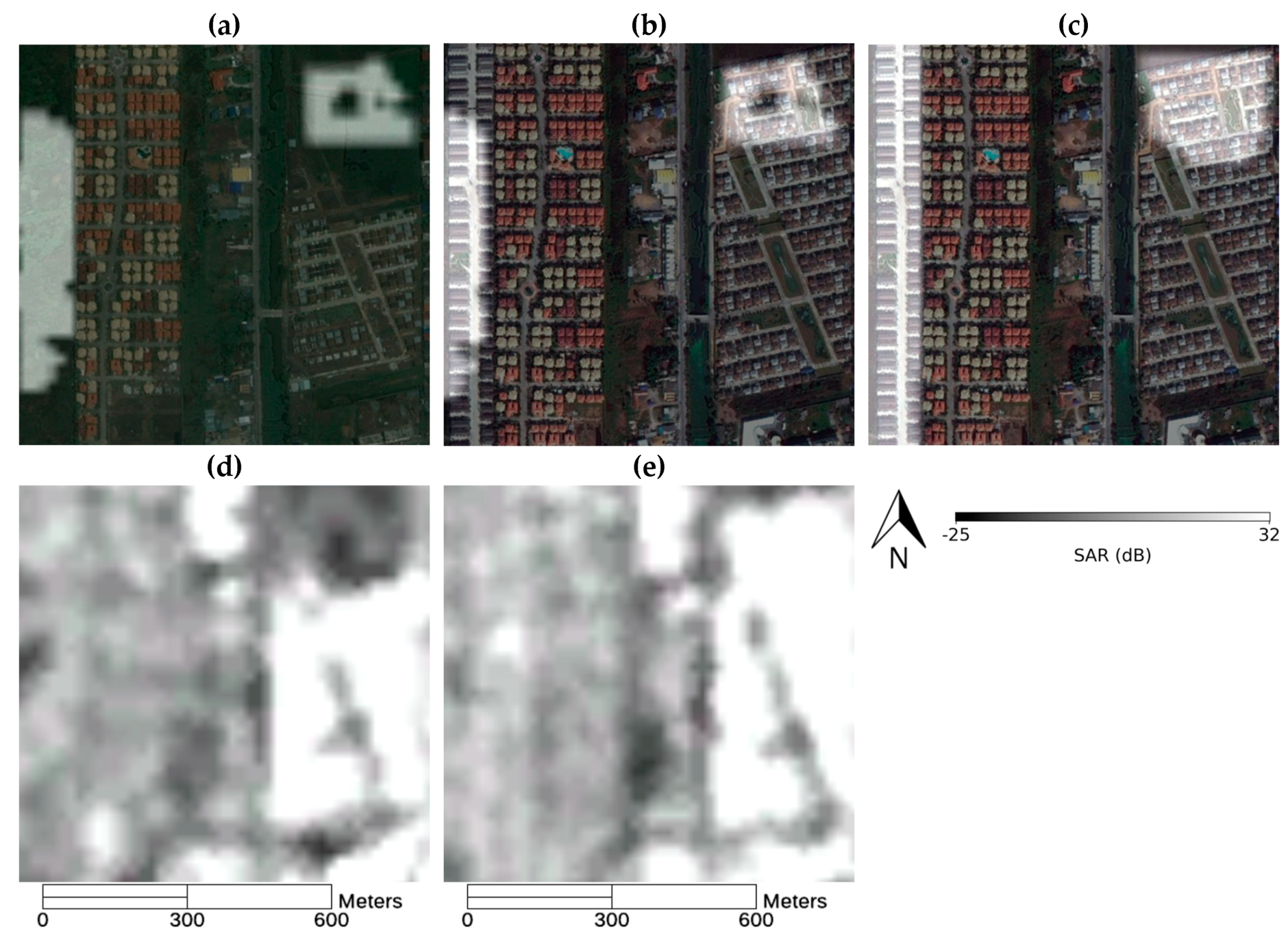
Figure 5.
Optical image showing an example of new constructions of Xiamen testing area. The size of (a) and (b) image are 3.7 × 2.8 km and size of (c) and (d) image are 1.7 × 1.7 km. (a) Time 1 image of first testing area from 12 May 2006, (b) Time 2 image of first testing area from 29 October 2009, (c) Time 1 image of second testing area from 5 December 2006, (d) Time 2 image of second testing area from 17 September 2011.
Figure 6.
Optical image showing an example of the new constructions in the Chiang Mai testing area. The size of each image is 3.77 km × 3.97 km. (a) Time 1 image from 17 November 2015, (b) Time 2 image from 24 December 2017.
Figure 6.
Optical image showing an example of the new constructions in the Chiang Mai testing area. The size of each image is 3.77 km × 3.97 km. (a) Time 1 image from 17 November 2015, (b) Time 2 image from 24 December 2017.
Figure 7.
Results of the Bangkok site in the first area of the SAR pair of 12 January 2009/21 November 2009, where the size of each image is 6 × 6 km: (a) the encoder 8 portion is 6:4, (b) the encoder 8 portion is 7:3, (c) the encoder 8 portion is 8:2, (d) the encoder 8 portion is 9:1, (e) ground truth. 14°1’2.26”N 100°41’15.99”E.
Figure 8.
Results of the Bangkok site in the second area of the SAR pair of 12 January 2009/21 November 2009, where the size of each image is 6 × 6 km: (a) Additional skip connection on one side of the network; (b) Additional skip connection on both sides of the network, (c) ground truth.
Figure 8.
Results of the Bangkok site in the second area of the SAR pair of 12 January 2009/21 November 2009, where the size of each image is 6 × 6 km: (a) Additional skip connection on one side of the network; (b) Additional skip connection on both sides of the network, (c) ground truth.
Figure 9.
Results of the Bangkok site in the first area at 14°1’2.26”N 100°41’15.99”E. The size of each image is 6 × 6 km (for SAR pairs 27 November 2008/15 January 2010: (a) Time 1 SAR image; (b) Time 2 SAR image; (c) ground truth; (d) result of U-net; (e) proposed result).
Figure 9.
Results of the Bangkok site in the first area at 14°1’2.26”N 100°41’15.99”E. The size of each image is 6 × 6 km (for SAR pairs 27 November 2008/15 January 2010: (a) Time 1 SAR image; (b) Time 2 SAR image; (c) ground truth; (d) result of U-net; (e) proposed result).
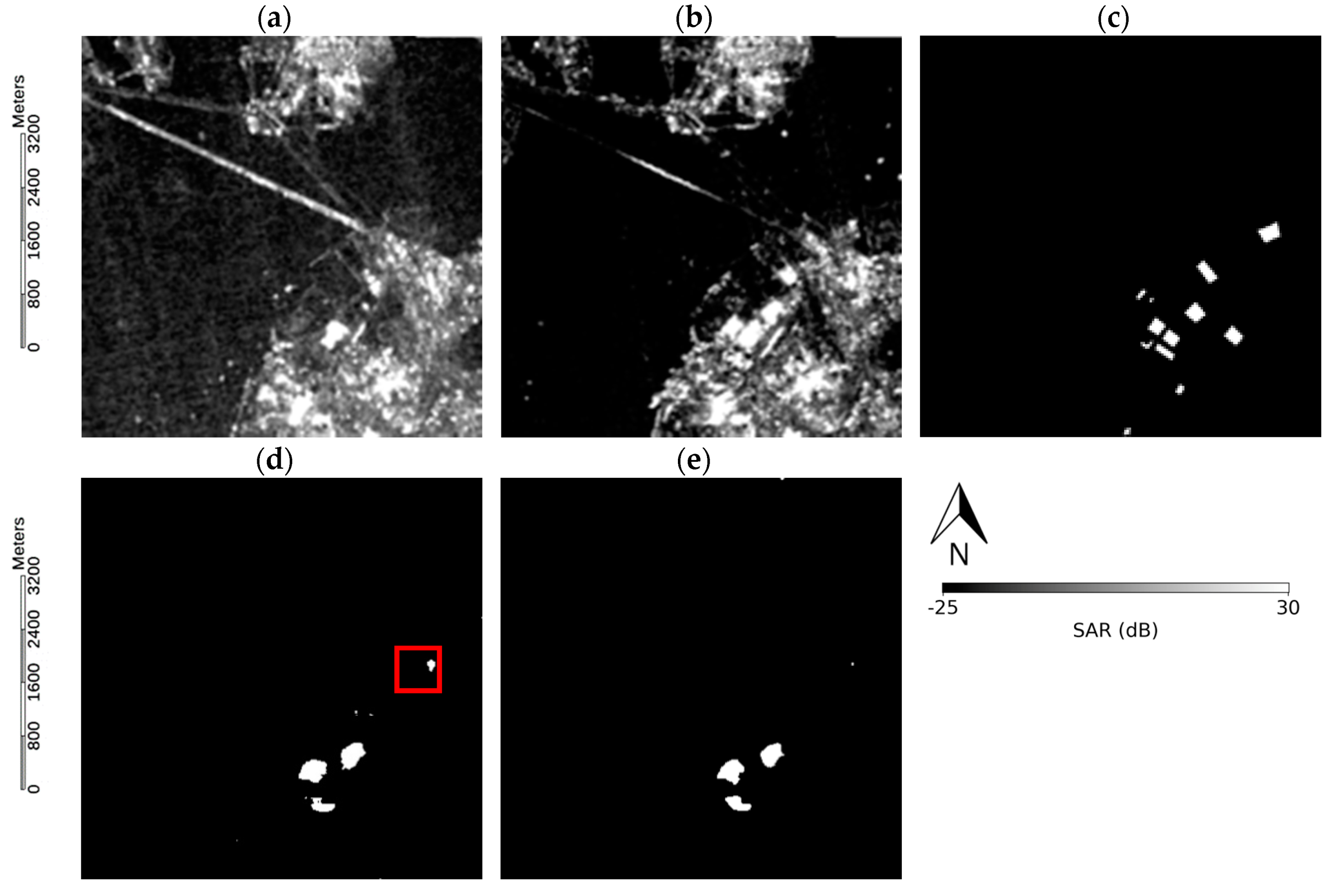
Figure 10.
Results of the Bangkok site in the first area at 14°1’2.26”N 100°41’15.99”E. The size of each image is 6 × 6 km (for SAR pairs 12 January 2009/21 November 2009: (a) Time 1 SAR image; (b) Time 2 SAR image; (c) ground truth; (d) result of U-net; (e) proposed result).
Figure 10.
Results of the Bangkok site in the first area at 14°1’2.26”N 100°41’15.99”E. The size of each image is 6 × 6 km (for SAR pairs 12 January 2009/21 November 2009: (a) Time 1 SAR image; (b) Time 2 SAR image; (c) ground truth; (d) result of U-net; (e) proposed result).
Figure 11.
Result of the Hanoi site at 20°57′06.35”N 105°51′08.87”E. The size of each image is 6 × 6 km. (a) Time 1 SAR data; (b) Time 2 SAR data; (c) ground truth; (d) result of proposed model; (e) result of U-net.
Figure 11.
Result of the Hanoi site at 20°57′06.35”N 105°51′08.87”E. The size of each image is 6 × 6 km. (a) Time 1 SAR data; (b) Time 2 SAR data; (c) ground truth; (d) result of proposed model; (e) result of U-net.
Figure 12.
Result of the first Xiamen test site at 24°28′35.28”N 118°11′36.12”E. The size of each image is 6 × 6 km. (a) Time 1 SAR data; (b) Time 2 SAR data; (c) ground truth; (d) result of proposed model; (e) result of U-net.
Figure 12.
Result of the first Xiamen test site at 24°28′35.28”N 118°11′36.12”E. The size of each image is 6 × 6 km. (a) Time 1 SAR data; (b) Time 2 SAR data; (c) ground truth; (d) result of proposed model; (e) result of U-net.
Figure 13.
Result of the second Xiamen test site at 24°31′59.42”N 118°06′54.51”E. The size of each image is 6 × 6 km. (a) Time 1 SAR data; (b) Time 2 SAR data; (c) ground truth; (d) result of proposed model; (e) result of U-net.
Figure 13.
Result of the second Xiamen test site at 24°31′59.42”N 118°06′54.51”E. The size of each image is 6 × 6 km. (a) Time 1 SAR data; (b) Time 2 SAR data; (c) ground truth; (d) result of proposed model; (e) result of U-net.
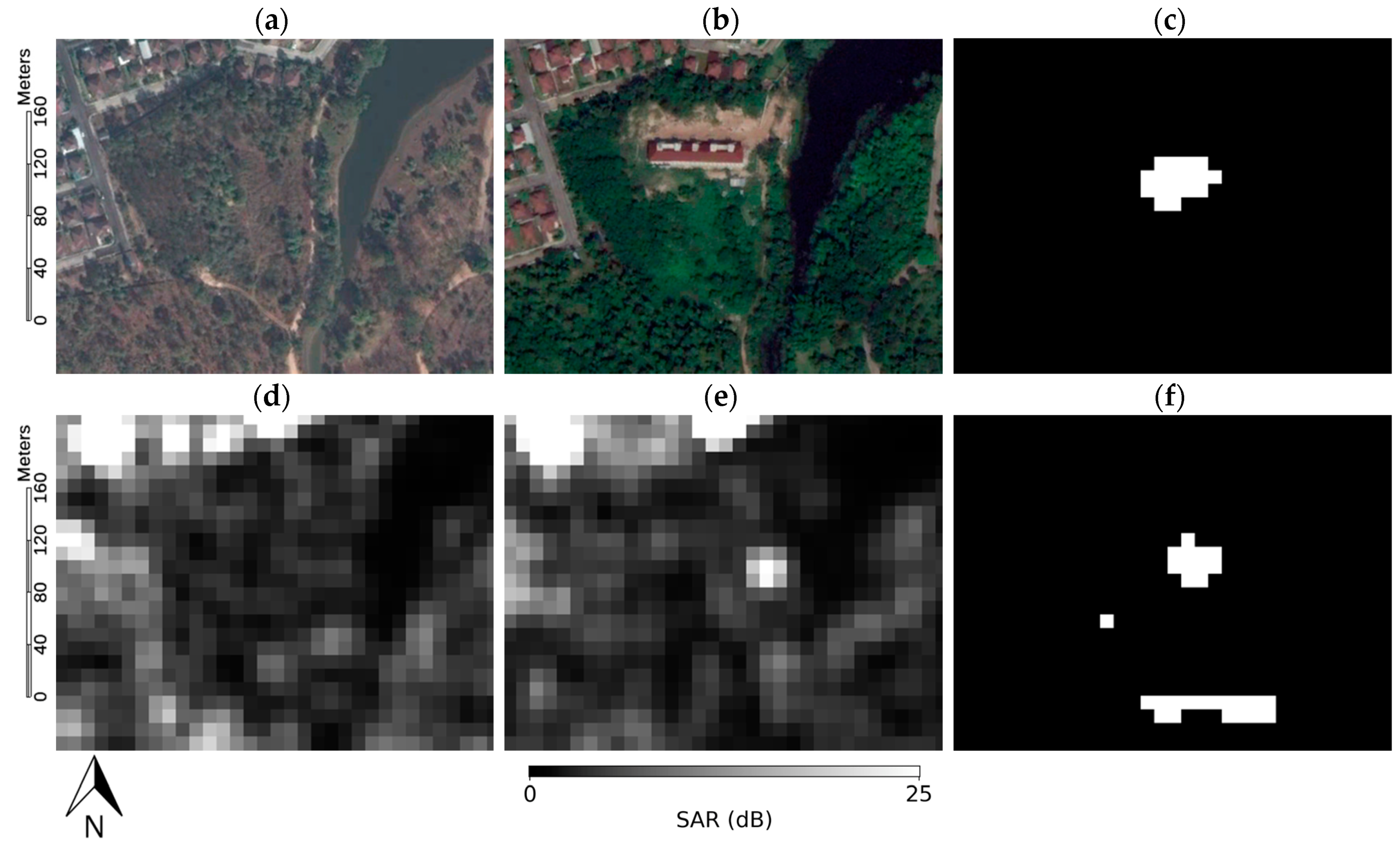
Figure 14.
Detection results of the first area in Chiang Mai at 18°51’23.49”N 98°57’17.90”E. The size of each image is 0.32 × 0.23 km. (a) Time 1 optical data; (b) Time 2 optical data; (c) result of CORN; (d) Time 1 SAR data ‘Copernicus Sentinel data [2015]’; (e) Time 2 SAR data ‘Copernicus Sentinel data [2017]’; (f) result of U-net.
Figure 15.
Detection results of the second area in Chiang Mai at 18°51’22.36”N 98°57’40.70”E. The size of each image is 0.32 × 0.23 km. (a) Time 1 optical data; (b) Time 2 optical data; (c) result of CORN; (d) Time 1 SAR data ‘Copernicus Sentinel data [2015]’; (e) Time 2 SAR data ‘Copernicus Sentinel data [2017]’; (f) result of U-net.
Figure 16.
The result of the proposed model with an image from Sentinel-1 at 18°50’48.34”N 98°56’55.95”E. The size of each image is 0.8 × 1.75 km. (a) Time 1 optical data; (b) Time 2 optical data; (c) Time 1 SAR data ‘Copernicus Sentinel data [2015]’; (d) Time 2 SAR data ‘Copernicus Sentinel data [2017]’; (e) result of CORN; (f) result of U-net.
Figure 17.
Optical image of the second area in Chiang Mai on 3 March 2018 at 18°51’22.36”N 98°57’40.70”E.
Figure 17.
Optical image of the second area in Chiang Mai on 3 March 2018 at 18°51’22.36”N 98°57’40.70”E.
Figure 18.
Example of detection results of CORN at Bangkok testing site for SAR pairs 12 January 2009/21 November 2009. (a) CORN result overlays on Time 1 optical image, (b) CORN result overlays on Time 2 optical image, (c) ground truth overlays on Time 2 optical image, (d) Time 1 SAR image, (e) Time 2 SAR image.
Figure 19.
Example of detection results of CORN at Hanoi testing site. (a) CORN result overlays on Time 1 optical image, (b) CORN result overlays on Time 2 optical image, (c) ground truth overlays on Time 2 optical image, (d) Time 1 SAR image, (e) Time 2 SAR image.
Figure 19.
Example of detection results of CORN at Hanoi testing site. (a) CORN result overlays on Time 1 optical image, (b) CORN result overlays on Time 2 optical image, (c) ground truth overlays on Time 2 optical image, (d) Time 1 SAR image, (e) Time 2 SAR image.
Figure 20.
Example of detection results of CORN at Xiamen testing site. (a) CORN result overlays on Time 1 optical image, (b) CORN result overlays on Time 2 optical image, (c) ground truth overlays on Time 2 optical image, (d) Time 1 SAR image, (e) Time 2 SAR image.
Figure 20.
Example of detection results of CORN at Xiamen testing site. (a) CORN result overlays on Time 1 optical image, (b) CORN result overlays on Time 2 optical image, (c) ground truth overlays on Time 2 optical image, (d) Time 1 SAR image, (e) Time 2 SAR image.
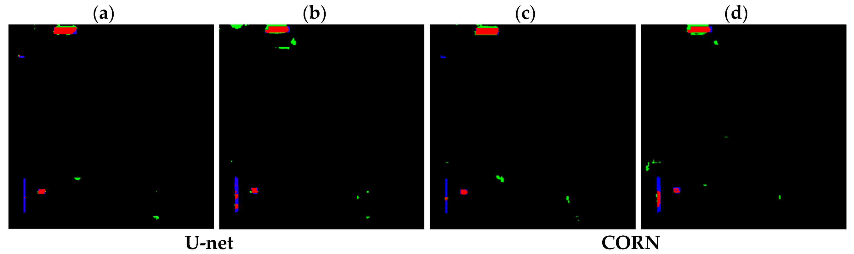
Figure 21.
Comparison of the proposed model’s result and the ground truth of the Bangkok testing site: (a) result of U-net for the SAR pair of 27 November 2008/15 January 2010; (b) result of U-net for the SAR pair of 12 January 2009/21 November 2009; (c) result of CORN for the SAR pair of 27 November 2008/15 January 2010; (d) result of CORN for the SAR pair of 12 January 2009/21 November 2009 ((red—true positive area; green—false positive area, blue—false negative area). The size of each image is 6 × 6 km.
Figure 22.
Detection results of CORN in the first area of Chiang Mai at 18°51’23.49”N 98°57’17.90”E in yellow hollowed polygon overlays on (a) a Time 2 optical images; (b) a Time 1 SAR image ‘Copernicus Sentinel data [2015]’ and (c) a Time 2 SAR image ‘Copernicus Sentinel data [2017]’.
Figure 22.
Detection results of CORN in the first area of Chiang Mai at 18°51’23.49”N 98°57’17.90”E in yellow hollowed polygon overlays on (a) a Time 2 optical images; (b) a Time 1 SAR image ‘Copernicus Sentinel data [2015]’ and (c) a Time 2 SAR image ‘Copernicus Sentinel data [2017]’.
Table 1.
Detail of the encoder and the decoder.
Table 1.
Detail of the encoder and the decoder.
| Encoder | Decoder |
|---|
| PCR (256,2,4,2) | CRD (1,512,2,2) |
| PCBR (128,64,4,2) | CRD (2,1024,2,2) |
| PCBR (64,128,4,2) | CRD (4,1024,2,2) |
| PCBR (32,256,4,2) | CRD (8,1024,2,2) |
| PCBR (16,512,4,2) | CRD (16,1024,2,2) |
| PCBR (8,512,4,2) | CRD (32,512,2,2) |
| PCBR (4,512,4,2) | CRD (64,256,2,2) |
| PCBR (2,512,4,2) | C (128,128,2,2) |
Table 2.
Acquisition information of dataset. SAR—synthetic-aperture radar.
Table 2.
Acquisition information of dataset. SAR—synthetic-aperture radar.
| Purpose | Location | Acquisition Date of SAR Images (Time 1–Time 2) | Acquisition Satellite | Resolution(meters) |
|---|
| Training | Bangkok, Thailand | 1 January 2008–15 January 2010 | ALOS-PALSAR | 15 |
| 12 January 2009–15 January 2010 | ALOS-PALSAR | 15 |
| | 1 January 2008–12 January 2009 | ALOS-PALSAR | 15 |
| Testing | Bangkok, Thailand | 27 November 2008–15 January 2010 | ALOS-PALSAR | 15 |
| 12 January 2009–21 November 2009 | ALOS-PALSAR | 15 |
| Hanoi, Vietnam | 2 February 2007–13 February 2011 | ALOS-PALSAR | 15 |
| Xiamen, China | 22 January 2007–2 November 2010 | ALOS-PALSAR | 15 |
| Chiang Mai, Thailand | 9 December 2015–24 December 2017 | Sentinel-1 | 10 |
Table 3.
The calculation of each validation method. IOU—intersect over union; TP–true positive; TN–true negative.
Table 3.
The calculation of each validation method. IOU—intersect over union; TP–true positive; TN–true negative.
| Validation Method | Calculation |
|---|
| Overall accuracy | |
| Precision | |
| Recall | |
| F measure | |
| F1 measure | |
| Kappa | |
| IOU | |
Table 4.
Accuracy of the model in the different encoder 8 portions at the Bangkok site.
Table 4.
Accuracy of the model in the different encoder 8 portions at the Bangkok site.
| Validation Method | 6:4 | 7:3 | 8:2 | 9:1 |
|---|
| False negative | 47.368 | 54.667 | 55.739 | 59.621 |
| False positive | 0.601 | 0.210 | 0.391 | 0.285 |
| Overall accuracy | 98.928% | 99.791% | 99.614% | 99.717% |
| Precision | 0.471 | 0.687 | 0.535 | 0.590 |
| Recall | 0.526 | 0.453 | 0.442 | 0.404 |
| F measure | 0.475 | 0.659 | 0.526 | 0.568 |
| F1 measure | 0.497 | 0.546 | 0.484 | 0.479 |
| Kappa | 0.492 | 0.543 | 0.480 | 0.475 |
| IOU | 0.331 | 0.376 | 0.320 | 0.315 |
Table 5.
Accuracy of the model in the different skip connections in the architecture at the Bangkok site.
Table 5.
Accuracy of the model in the different skip connections in the architecture at the Bangkok site.
| Validation Method | Proposed Network | Additional Skip Connection on Both Sides |
|---|
| False negative | 54.667 | 66.936 |
| False positive | 0.210 | 0.180 |
| Overall accuracy | 99.791% | 99.149% |
| Precision | 0.687 | 0.652 |
| Recall | 0.453 | 0.331 |
| F measure | 0.659 | 0.603 |
| F1 measure | 0.546 | 0.439 |
| Kappa | 0.543 | 0.435 |
| IOU | 0.376 | 0.281 |
Table 6.
Accuracy of the model in the Bangkok area.
Table 6.
Accuracy of the model in the Bangkok area.
| Validation Method | Proposed Network | U-net |
|---|
| False negative | 54.667 | 55.801 |
| False positive | 0.210 | 0.403 |
| Overall accuracy | 99.791% | 99.04% |
| Precision | 0.687 | 0.527 |
| Recall | 0.453 | 0.442 |
| F measure | 0.659 | 0.519 |
| F1 measure | 0.546 | 0.481 |
| Kappa | 0.543 | 0.476 |
| IOU | 0.376 | 0.316 |
Table 7.
Accuracy of the model in the Hanoi area.
Table 7.
Accuracy of the model in the Hanoi area.
| Validation Method | Proposed Network | U-net |
|---|
| False negative | 62.980 | 58.324 |
| False positive | 0.782 | 0.922 |
| Overall accuracy | 99.522% | 98.77% |
| Precision | 0.204 | 0.196 |
| Recall | 0.370 | 0.417 |
| F measure | 0.211 | 0.205 |
| F1 measure | 0.263 | 0.267 |
| Kappa | 0.258 | 0.261 |
| IOU | 0.151 | 0.154 |
Table 8.
Accuracy of the model in the Xiamen area.
Table 8.
Accuracy of the model in the Xiamen area.
| Validation Method | Proposed Network | U-net |
|---|
| False negative | 68.652 | 77.577 |
| False positive | 0.861 | 0.508 |
| Overall accuracy | 98.189% | 98.412% |
| Precision | 0.341 | 0.385 |
| Recall | 0.313 | 0.224 |
| F measure | 0.338 | 0.364 |
| F1 measure | 0.327 | 0.283 |
| Kappa | 0.317 | 0.276 |
| IOU | 0.195 | 0.165 |
Table 9.
Accuracies of the models in the different number of training data at the Bangkok site.
Table 9.
Accuracies of the models in the different number of training data at the Bangkok site.
| Validation Method | 500 Pairs | 1500 Pairs |
|---|
| CORN | U-net | CORN | U-net |
|---|
| False negative | 40.860 | 27.512 | 53.254 | 47.232 |
| False positive | 1.467 | 17.970 | 0.383 | 0.683 |
| Overall accuracy | 98.136% | 81.934% | 99.085% | 98.848% |
| Precision | 0.310 | 0.100 | 0.590 | 0.492 |
| Recall | 0.591 | 0.725 | 0.467 | 0.528 |
| F measure | 0.321 | 0.107 | 0.571 | 0.488 |
| F1 measure | 0.400 | 0.165 | 0.507 | 0.485 |
| Kappa | 0.391 | 0.150 | 0.503 | 0.480 |
| IOU | 0.251 | 0.092 | 0.340 | 0.321 |

 and
and 


