Abstract
It is important to grasp the number and location of trees, and measure tree structure attributes, such as tree trunk diameter and height. The accurate measurement of these parameters will lead to efficient forest resource utilization, maintenance of trees in urban cities, and feasible afforestation planning in the future. Recently, light detection and ranging (LiDAR) has been receiving considerable attention, compared with conventional manual measurement techniques. However, it is difficult to use LiDAR for widespread applications, mainly because of the costs. We propose a method for tree measurement using 360° spherical cameras, which takes omnidirectional images. For the structural measurement, the three-dimensional (3D) images were reconstructed using a photogrammetric approach called structure from motion. Moreover, an automatic tree detection method from the 3D images was presented. First, the trees included in the 360° spherical images were detected using YOLO v2. Then, these trees were detected with the tree information obtained from the 3D images reconstructed using structure from motion algorithm. As a result, the trunk diameter and height could be accurately estimated from the 3D images. The tree detection model had an F-measure value of 0.94. This method could automatically estimate some of the structural parameters of trees and contribute to more efficient tree measurement.
1. Introduction
Obtaining tree metrics has various applications in fields such as commercial forestry, ecology and horticulture. Tree structure measurement is fundamental for resource appraisal and commercial forest management [1]. In urban spaces, the knowledge of tree structure is important for their maintenance and for understanding their effects on urban environments. Trees in urban spaces have a significant influence upon urban environments through solar shading, transpiration, windbreaking, air purification and soundproofing [2]. Another important reason for measuring tree structure, including height and tree trunk diameter, is the creation of tree registries and regular monitoring for public safety. Therefore, trees in forests and cities play important roles, and the tree structural measurement is essential for their effective utilization.
The conventional method is manual, and the tree measurement should be conducted one by one, meaning that the measurement is very tedious and time consuming. Besides, the manual measurement cannot be done frequently due to the hardness of the experiment. Then, measurement using terrestrial light detection and ranging (LiDAR) has attracted considerable attention. LiDAR is a three-dimensional (3D) scanner that provides highly accurate and dense 3D point clouds. A terrestrial LiDAR, which is placed on the ground, has been used widely.
Previous studies on the LiDAR have estimated tree trunk diameter, tree height [3,4,5], leaf area density [6,7], tree volume [8], biomass and leaf inclination angle [9,10]. However, when we use a LiDAR that should be stationed at one point for the measurement, it can require multiple measurements to cover the study sites, depending on the scale and shape of the study site. Recently, a light weight and portable LiDAR has been used for tree measurement [11]. This LiDAR measurement can be conducted while moving, enabling large area-measurement in a short period. Moreover, the field of view of LiDAR is large when the measurement is carried out during movement, and the maximum distance for measurement is not short (e.g., 100 m). Those LiDAR instruments also can be utilized with unmanned aerial systems or drones [12,13,14]. By combining LiDAR with those platforms, the 3D data of large area including numerous trees can be easily obtained. However, the instrument is costly, and the measurement process, such as in forests, is laborious. Moreover, LiDAR itself cannot obtain the color value.
Structure from Motion (SfM) is a photogrammetric approach for 3D imaging, where the camera positions and orientations are solved automatically after extracting image features to recover 3D information [15]. Liang et al. [16] showed that the mapping accuracy of a plot level and an individual-tree level was 88 %, and the root mean squared error of the diameter at breast height (DBH) estimates of individual trees was 2.39 cm, which is acceptable for practical applications. Additionally, the results achieved using terrestrial LiDAR are similar. Piermattei et al. [17] concluded that the SfM approach was an accurate solution to support forest inventory for estimating the number and the location of trees. In addition, the DBHs and stem curve up to 3 m above the ground. Qiu et al. [18] developed a terrestrial photogrammetric measurement system for recovering 3D information for tree trunk diameter estimation. As a result, the SfM approach with a consumer-based, hand-held camera is considered to be an effective method for 3D tree measurement.
However, the field of view of cameras is limited, compared with LiDAR [19]. For example, to capture trees on the right and left side in the direction of movement, the measurement should be conducted at least twice for both sides. Moreover, a certain distance is necessary from the target to cover the whole tree. However, it is sometimes impossible to achieve this distance because of restrictions in the field.
Recently, 360° spherical cameras that capture images in all directions have been used widely. The field of view of the 360° spherical camera is omnidirectional, while that of the mobile LiDAR is not (e.g., Velodyne VLP-16: vertical ± 15°). In addition, color information can be obtained as well. Moreover, it is much lighter and inexpensive than LiDAR.
As mentioned, the 360° spherical camera has advantages of both a LiDAR and a camera. These are omnidirectional view, availability of color information, light weight and affordable cost. Further, 3D point clouds can be reconstructed from the spherical images using SfM [20,21]. A previous study estimated the sky view factor with the 360° spherical camera with color information. This sky view factor is a ratio of the sky in the upper hemisphere, and it is an important index in many environmental studies [22]. However, structural measurement via 3D imaging has not been explored thus far. Further, if structural measurement can be performed using a spherical camera, automatic tree detection, which leads to automatic tree analysis, is required. Automatic tree detection of each tree enables the estimation of properties such as tree trunk diameter and tree height. Two approaches for automatic tree detection from the spherical images can be considered. The first is to detect trees from the reconstructed 3D images using a 3D image processing technique. For example, a tree identification method with a cylinder or a circle fitting the tree trunk is used popularly [23,24]. As another method [25,26], it utilizes the intensity of the reflectance of the laser beam from the LiDAR for tree detection. However, 3D image processing requires considerable memory size, and the calculation cost tends to be large. In addition, when reconstructing 3D images using SfM, there are many missing points, owing to the absence of matching points among the input images around the missing area, and the mis-localized points. This makes it difficult to detect trees from 3D images.
The second approach is to detect trees in two-dimensional (2D) images and reconstruct the 3D images with the information of each tree identification. As mentioned above, if the 3D images recovered from SfM are not complete because of missing points, the resolution and accuracy of the input 2D images will be much higher than the reconstructed 3D images. Therefore, it is assumed that the detection from 2D images is more accurate than from 3D images. One of the biggest challenges in the tree detection from 2D images is the presence of numerous objects in the background. 2D image processing cannot utilize depth information, unlike 3D image processing. Recently, the methodology for detecting the target automatically has been rapidly improved, because of the use of a deep learning-based technique. A region-convolutional neural network (R-CNN) [27] applied deep learning for target detection for the first time. The traditional features are replaced by features extracted from deep convolution networks [28]. Fast R-CNN and Faster R-CNN have been developed for overcoming the disadvantages of the long processing time of R-CNN [29,30].
Nowadays, other algorithms for object detection are available, such as YOLO and SSD [31,32]. These methods operate at a very fast speed with high accuracy. The YOLO model processes images at more than 45 frames per second. The speed is increasing because the algorithm is being updated. Hence, real-time based detection is now possible. We used the YOLO v2 model [33], and the tree detector constructed based on YOLO v2 is called YO v2 detector in this paper.
In this study, the tree images were obtained with a 360° spherical camera, and its 3D reconstruction was done using SfM to estimate the tree trunk diameter and tree height. Next, the tree detector was developed based on the YOLO v2 network. The 3D point clouds were reconstructed with information from the tree detection. Finally, the trees in the 3D point clouds were automatically detected.
2. Materials and Methods
2.1. Plant Materials
The trees in the campus of the University of Tokyo, Japan, were selected for this study. The study site was full of green spaces and varieties of tree species. Examples of these are Yoshino cherry (Cerasus x yedoensis), Plane tree (Platanus), Japanese zelkova (Zelkova serrata), Ginkgo (Ginkgo biloba L.), Himalayan cedar (Cedrus deodara), Japanese false oak (Lithocarpus edulis), and Azelea (Rhododendron L.).
2.2. Tree Trunk Diameter and Tree Height Measurement
For the tree trunk diameter estimation with a 360° spherical camera, ginkgo trees were selected (n = 20). A vinyl rope was wound around the trunk of the tree, and the diameter was measured using a tree caliper. The diameter ranged from approximately 30 cm to 80 cm. For the height measurement, 20 trees with of height approximately 3–25 m were selected. For the tree height measurement, LiDAR (Velodyne VLP16, USA) was used. For the 3D reconstruction from LiDAR image, a SLAM technique by Zhang et al [34] called LOAM was used. The top and bottom points, which should be used for height measurement in the constructed LiDAR 3D images, were selected for height validation by visual observation.
2.3. Tree Measurement with 360° Spherical Camera and 3D Reconstruction
The 360° spherical camera used in this study was THETA V (Ricoh Company Ltd.) and THETA SC (Ricoh Company Ltd.) [35]. The camera THETA V and THETA SC can record a video with a resolution of 3840 × 1920 and 1920 × 1080, respectively. The video resolution will affect the quality of 3D images. The 360° spherical camera was attached to a Ricoh THETA stick [36], and the stick was hand-held while walking. The height of the camera was approximately 2 m. The images to be input for the 3D reconstruction were derived from the video frames. The walking speed was approximately 1 m/s, and the camera position was stable, resulting in no blurred images in the video frames.
The distance between the target and the camera was set at 4 m and 8 m, for the tree trunk diameter estimation. For the height measurement, the images were taken while walking for approximately 20 m.
The software used for 3D reconstruction was Agisoft Metashape (Agisoft LLC, Russia), which was formerly Agisoft Photoscan. Agisoft Metashape reconstructs 3D images from 2D input images after estimating the camera position and angle through image feature matching. Metashape creates highly dense 3D images by applying the latest multi-view algorithms into a series of overlapped images. The software is reviewed in a previous study [37].
The scale in the reconstructed 3D images was not determined with the input images solely. A reference scale, such as a big caliper or a part of a building, was determined, and the scale of the 3D image was calculated with the length of the reference. For the tree trunk diameter estimation, 60 and 120 images, respectively, from THETA V (video resolution: 3840 × 1920) and THETA SC (video resolution: 1920 × 1080) were used for 3D reconstruction. Eighty images were input from THETA V for the tree height estimation. To obtain the input images, one image per 10 frames and 5 frames was obtained from THETA V and SC, respectively.
2.4. Evaluating the Trunk Diameter and Height Estimation
Two points on the vinyl rope in the reconstructed 3D images, which corresponds to the tree trunk edge, were selected manually, and the distance was calculated. The difference between the estimated value and the measured value was then compared for estimating the tree trunk diameter. Also, the top point of the tree canopy was selected manually from the 3D images to estimate the tree height. Next, the estimated value was compared with the value derived from the LiDAR 3D image. The 3D point cloud images had some points that correspond to the tree trunk edge and the tree top point. This could result in handling errors during estimation. Therefore, the points were selected three times, and their mean value was used for the estimation.
2.5. About YOLO Detector
2.5.1. Overview of YOLO Detector
Figure 1 illustrates the overview of the YOLO detector. Here, YOLO v2 was used. The figure is obtained by modifying the image provided by Redmon et al [31]. The image is split into cells of S by S (in Figure 1a: 5 by 5). The next step is shown in panels [b] and [c]. The probability of the class in each grid, indicating that an object is included in that grid, is calculated. Then, each cell in panel [b] contains information of the class which the object in the cell belongs to. Based on the probability, the predicted class in each cell was illustrated by a different color. In panel [c], the confidence score, as shown in Eq. (1), and the bounding box, were calculated. The confidence score is a product of the conditional class probabilities and the intersection over union (IoU). For details, refer to [31].
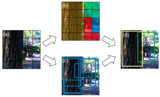
Figure 1.
Overview of the YOLO detector. Input images were divided into cells of S by S (a). In each cell, the class probability (b) and the information related to the location, size, and confidence score (c) were estimated. By considering the information in (b) and (c), the final object detection was done (d). We referred to and modified the figure of Redmon et al. [31] for this image.
In panel [d], the product of the confidence score and the class probability was calculated to obtain the final bounding box for detection.
However, multiple bounding boxes (more than one) per object were observed. To finalize the bounding box to represent each object, non-maximal suppression [38] was performed. For example, in Figure 2, Box 1 and Box 2 intersect. Intersection over union, as defined in Equation (2), was calculated. If the IoU value is more than 0.5, the box was eliminated. The bounding box with a higher score remains. Similarly, Box 4 was deleted.
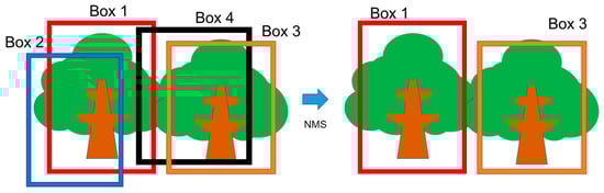
Figure 2.
Non-maximal suppression (NMS) for eliminating redundant bounding boxes. The two boxes with intersection over union (IoU) greater than 0.5 were focused upon. One box with a higher score remains, and the other was reduced.
2.5.2. Network Architecture
First, the YOLO detector extracts image features. The properties of the class of the grid and bounding box were predicted via the deep neural network. Information on the bounding box comprises the width, height and location (x, y). To construct the network from scratch is not easy. Hence, a pre-trained network was imported. ResNet-50 [39] was used for the pre-trained network, which performed image classification with a high accuracy, for an image dataset called ImageNet [40]. In the original paper on YOLO, a CNN inspired by GoogleNet [41] was prepared, and the network was trained using ImageNet. We followed this method and the pre-trained network, Reset-50 trained with ImageNet, was imported. This was implemented with Matlab 2019a (Mathworks, USA). Figure 3 summarizes the network architecture. The input size of image [a] in this network was 224 × 224 × 3, because the ResNet-50 accepts the only image size of 224 × 224 × 3. This “3” stands for red, green and blue channels.
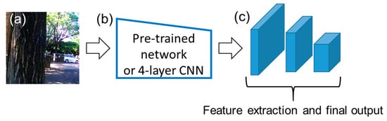
Figure 3.
Network architecture of YOLO. Panel (a) represents the input image. The input images were processed using convolutional operations in the convolutional neural networks (CNNs), as in (b) and (c). The network structure and initial values were imported from a pre-trained network, ResNet-50. The layers from the first to the 141st were used. The input size was 224 by 224 with the RGB channel. Then, a CNN containing three convolutional layers was connected, and the final output was obtained. Added to ResNet-50, a CNN with four layers was used for network [b]. The input size was 252 by 252.
The 141st layer in ResNet-50 was the rectified linear unit (ReLu) layer, and its output size was 14 × 14 × 1024. The ResNet-50 structure from the first to the 141st layer has been utilized, as shown in panel [b]. Herein, the network in Figure 3 [b] was called by the feature extractor; however, the weights and biases were updated throughout the training process. After obtaining the output of 14 × 14 × 1024 from the ResNet-50 based network, the features for the final output were extracted as shown in [c]. The CNN-based network was prepared and directly connected to the end of the network of panel [b]. It was also built by the CNN-based network, comprising three convolutional layers, batch normalization layers and ReLu layers [c]. The final output is the information on the class of each grid, location of the object and confidence of the estimation.
Additionally, instead of ResNet-50, a simple CNN with four layers was also used. The CNN comprises a convolution layer, batch normalization layer, max pooling layer, ReLu layer, fully connected layer and softmax layer. The initial values of the weights in the convolutional and fully connected layers were determined based on [42]. The input size of the image was 252 × 252 × 3.
2.5.3. Anchor Box
In YOLO v2, the anchor box was introduced [33]. The final output in Figure 3c does not regress the location of the bounding boxes directly. As shown in Figure 4, the boxes called anchor boxes are tiled throughout the image. In the final output, the difference in the size and location between the tiled anchor box and the estimated bounding box was predicted. Here, the difference in the location was determined as follows: for the calculation, the position of the x and y values of the center of bounding boxes, and the position of the x and y values of the center of anchor boxes was used. Then, the distance of the two center positions was calculated for determining the difference. Also, the difference in the width and height from the anchor box was estimated. The localization of the anchor box and the size of the final feature map obtained in Figure 3c are identical. If the size of the final feature map is 5 × 5, the localization of the anchor box is also 5 × 5. Here, the size of the anchor box can be a parameter for training the YOLO v2 detector. The number of anchor boxes are optional, where the higher number of anchor boxes translates to a higher object identification ability, with longer processing and prediction times. The manner in which the number and size of the anchor boxes were determined is explained in Section 2.7.
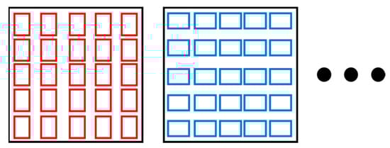
Figure 4.
Anchor boxes for object detection. The number of anchor boxes corresponds to the number of grids in Figure 1a. The number and size of the anchor boxes was pre-determined. In interference, the location and size of the detected objects were denoted using the difference from the location and the size of the anchor boxes.
2.5.4. Cost Calculation
The YOLO v2 network for object detection optimizes the mean squared error (MSE) loss between the properties of the bounding box and the class of the correct label and its prediction. The loss function can be given as follows [43]:
where is the total loss. , and are the losses in the bounding box, confidence score, and class probability estimation, respectively. The loss regarding bounding box () comprises four errors: errors of the coordinates of the center of the bounding box (x, y), and error of the length of the bounding box (width and height). This loss was evaluated based on the pre-determined bounding boxes that were made manually, for the training and test samples, as shown in Section 2.6.1. Their loss can be weighed using parameters , and . The parameter setting is described in Section 2.6.3. The loss, can be divided into two parts; however, it has been combined here.
2.5.5. Number of Grid Cells and Output Sizes of the Final Feature Map is Determined
In this study, YOLO v2 was done in Matlab 2019a (Mathworks, USA). The detailed description on YOLO v2 below is based on how Matlab runs. The output size of the pre-trained network based on ResNet-50, as shown in Figure 3b, was 14 × 14 × 1024. The convolutional filters of the CNN shown in Figure 3c had a stride of 1. When convoluting pixels around the edges, padding was done so that the output had the same size as the input. Here, the height and width of the feature map after convolution was 14. Therefore, the grid size as shown in Figure 1a was 14 × 14. The number of grid cells was determined by the CNN architecture. The height and width of the final feature map and the number of the grid cells was identical. For example, if the value of stride of the convolutional filter increased in the network Figure 3c, the height and width of the final feature map decreased, resulting in fewer grid cells in Figure 1a.
2.5.6. Dimensions of Final Feature Map
As mentioned, the indices predicted by the YOLO v2 network are the offsets of the anchor boxes, regarding the center of the bounding box (x, y), the height and width, confidence score and conditional class probability. If the number of objects that can appear in the image is three (class A, B, and C), three values of class probability corresponding to each class should be estimated. Thus, a total of 8 (4 + 1 + 3) values in each cell should be estimated. Then, the size of the final feature map will be 14 × 14 × 8 when the number of anchor boxes is 1. The indices above were estimated for each anchor box independently. This implies that if the number of anchor boxes is four, the size becomes 14 × 14 × 32. Thus, the greater the number of anchor boxes prepared, the higher the accuracy of object detection, with increasing processing time.
2.6. Training the YOLO v2 Detector
2.6.1. Training and Test Dataset
Videos of the trees in the study site were recorded using THETA SC. The training and test images were retrieved by dividing the videos into image frames. Training with all the frames from the videos increases the training time. Therefore, the frames used were determined randomly.
In total, 799 images were obtained, and the labeling for the training and test was done manually, as shown in Figure 5. The images dataset after labeling were divided into training and test datasets, in a ratio of 9:1.
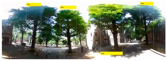
Figure 5.
Example of labeling for object detection. This image was derived from video frames, and the trees in the video were labeled with bounding box manually.
2.6.2. Pre-Training of the Feature Extractor in YOLO v2 Detector
Pre-training for the feature extractor, as shown in Figure 3b, was performed. That is, the initial values in ResNet-50 and the 4-layer network were changed to increase the accuracy of the YOLO v2 detector. ResNet-50 was to be transferred for the future extractor, as shown in Figure 3b. The weight and bias values were obtained by training the images in ImageNet [40], and not for the tree recognition. Then, the transferred network was tuned by solving an image classification problem, to optimize the initial values of the feature extractor as mentioned below. In addition, the 4-layer network shown in Figure 3 does not undergo any training. It was assumed that if the 4-layer network is pre-trained to extract the good features of trees, the detection accuracy could be increased. Then, the initial values of the 4-layer network were tuned by solving the image classification problem as shown below.
The images that contain trees and those that do not contain any trees were obtained by the 360° spherical camera. They were not included in the training and test dataset for the YOLO v2 detector. The binary classification into either a tree image or a non-tree image was done. The number of training and test images were 400 and 100, respectively. The ratio of each class was the same. In this training, 60 validation images were prepared, which were different from the training and test images to determine the parameters for training. The classification accuracy was calculated after every three iterations. When the validation loss was larger than or equal to the previous smallest loss for three consecutive iterations, the training process was stopped (early stopping) [44,45].
Figure 6 shows the training technique for the binary classification of the tree and non-tree images with ResNet-50 and the 4-layer network. ResNet-50 and the 4-layer network were trained using the training data of the tree and non-tree images. The constructed network was used for the feature extractor, as shown in Figure 3b. This changed the weight and bias values in ResNet-50. The parameters for binary classification are listed in Table 1. The accuracy of YOLO v2 with and without the optimization of this initial value of the pre-trained network was compared.
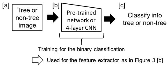
Figure 6.
Training for the feature extractor for YOLO v2 detector. The input images were tree or non-tree images [a]. Pre-trained network and 4-layer CNN [b] were trained with the images to classify into tree or non-tree [c]. Then, the weights of the networks were used for the feature extractor in the YOLO network.

Table 1.
Parameters for binary classification of tree/non-tree images. SGD in the optimizer stands for stochastic gradient decent.
2.6.3. Determination of the Number and Size of the Anchor Box and Other Parameters
Next, the number and size of the anchor boxes was determined based on the labels included in the training data, as discussed in Section 2.6.1. A method proposed in a previous study was used for this determination [33]. First, the heights and widths of the bounding box included in the training data were listed. Then, the pair of width and height was clustered based on IoU, as in Equation (2). To calculate IoU, two boxes were positioned as shown in Figure 7, and the (x, y) coordinate of the centroid of each bounding box was not considered to focus on the width and height.
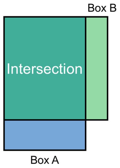
Figure 7.
Positioning of bounding boxes for the intersection over union (IoU) calculation. The bounding boxes are those included in the training dataset. Based on this position, IoU with bounding box A and B was calculated, and the result was used for the clustering in the next step.
Next, the pairs of the heights and widths of the bounding boxes were clustered using the K-medoids algorithm [46]. The clustering algorithm such as K-means and K-medoid are run using the distance between each data. Here, the distance was defined as shown in Eq. 4, instead of the Euclidean distance.
The distance was based on IoU, which implies that the bounding boxes that cover similar areas should be in the same group. In the clustering algorithms, a pair of data with small distance should be in the same group. However, with increased similarity in the properties of the bounding boxes, the IoU value increases with the maximum of 1. Hence, the distance was defined after reducing from 1, as in Equation (4). Here, the list of bounding box properties was clustered in groups of eight to determine the width and height of the eight bounding boxes. Figure 8 represents the clustering results based on the IoU value between bounding boxes. The horizontal and vertical axis in Figure 8 shows the area and aspect ratio of the bounding box.
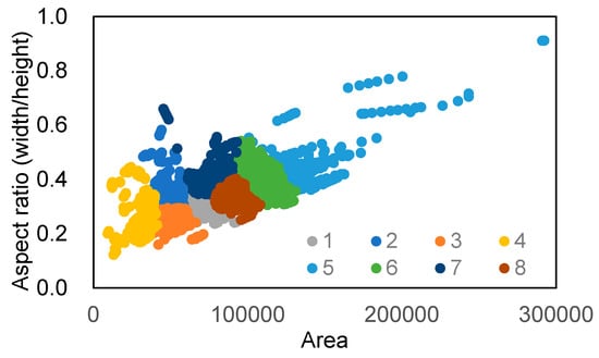
Figure 8.
Clustering result of bounding boxes included in the training dataset. Each plot in this figure corresponds to each bounding box. Each plot was clustered using the K-medoids algorithm based on the distance defined in Equation (4).
The area was calculated based on the pixel number of the height and width of the bounding boxes. Note that the clustering result was obtained with the IoU, and the values of the x and y axis were not directly used for clustering.
For training the YOLO v2 detector, the weights of K1, K2 and K3 in the loss function shown in Equation (3) were set to 5, 1 and 1, respectively. The training parameters for YOLO v2 detector are listed in Table 2. The workstation used for the calculation for training and 3D reconstruction, using SfM, was DELL Precision T7600. The CPU was Xeon E5-2687w, 3.1GHz, the RAM was 64 GB, and the GPU was Quadro K5000.
Table 2.
Parameters for training the YOLO v2 detector. The optimizer was the aforementioned stochastic gradient decent (SGD) with momentum.
The processing times of the YOLO v2 detector with the ResNet-50 and 4-layer network were compared. The inference with 80 images was demonstrated individually, and the processing time per image was calculated. The PC for this inference was Let’s note CF-SV8KDPQR (Panasonic, Japan), with Intel Core i5-8265U CPU. The RAM and Processor Base Frequency were 16 GB and 1.6 GHz, respectively.
2.7. Post Processing after 3D Reconstruction
After reconstructing the 3D images using SfM with the information obtained on tree detection, post processing was conducted to separate each tree. Here, the trees in the 360° spherical images were detected using the YOLO v2 detector, which was trained with ResNet-50 without pre-training. Figure 9 shows the overview of the post-processing of the reconstructed 3D images. This method is referred to as Itakura and Hosoi [47,48]. First, the 3D images were reconstructed with the information of the tree in panel [a].
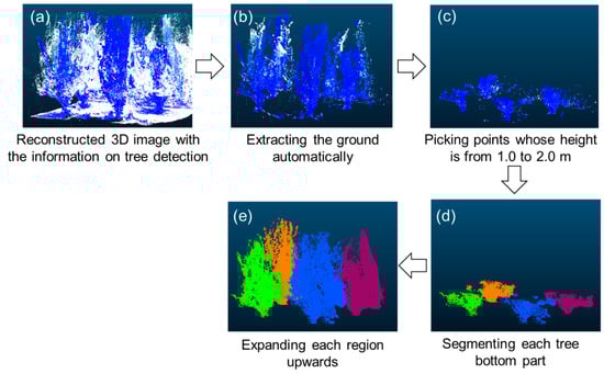
Figure 9.
Overview of the post-processing of 3D images reconstructed using Structure from Motion (SfM). This method referred to previous methods [47,48]. Panel (a) shows the reconstructed 3D image with the information of “tree”, as predicted by the YOLO v2 detector. The point indicated by blue corresponds to the tree point. Then, the ground was automatically reduced using the Maximum Likelihood Estimation Sample and Consensus (MLESAC) algorithm [49] as shown in the panel (b). Next, the points with the heights of 1.0–2.0 m were extracted (c). Then, the points within 30 cm were clustered into the same group (d). Finally, each tree could be segmented after expanding each region into the upper direction (e).
The points with the label “tree” are illustrated in blue. The xyz value (unit: meter) was rounded to one decimal place to reduce the number of points in the 3D images. Next, the ground was automatically removed using the Maximum Likelihood Estimation Sample and Consensus (MLESAC) algorithm [49], as shown in panel [b]. The noises included in the 3D images were excluded based on the density [50]. Then, the points with height of 1.0–2.0 m with the label “tree” were selected [c]. The clusters were considered as tree trunks and the lower part of tree canopies. Here, the cluster with less than 100 points was excluded. The maximum distance among all the points included in each cluster was calculated. If the distance was greater than 3 m, the cluster was also reduced, because the cluster is unlikely to be a tree trunk and more likely to be a wall or other object. The points with distances within 30 cm were clustered into the same group [d]. By expanding the region upwards, each tree could be detected. In this expanding process, only the points that can be considered as leaves were considered. The point with the G/R value greater than 1.2, or the point assigned to the tree by the YOLO v2 detector was used for expansion. Automatic tree detection was done with video frames not included either in the training or the test dataset. In total, 69 trees were tested for detection.
3. Results
3.1. Tree Trunk Diameter and Height Estimation
The video recorded by THETA V had a resolution of 3840 × 1920. The mean absolute error of the tree trunk diameter estimation was approximately 2.6 2.3 and 2.8 2.6 cm, when the distance between the camera and the tree was 4 m and 8 m, respectively. The mean absolute error with THETA SC, whose resolution was 1920 × 1080, was approximately 5.0 4.4 and 4.4 3.7 cm, when the distance was 4 m and 8 m, respectively.
The absolute error of the estimated tree height was approximately 58.1 62.7 cm. In all samples, the tree trunk could be reconstructed in 3D images. However, certain trunks, particularly those from THETA SC, were sometimes unclear, resulting in a higher estimation error.
3.2. Automatic Tree Detection
3.2.1. Pre-Training of the Feature Extractor of YOLO v2 Detector
Binary classification of tree and non-tree objects was carried out to pre-train the feature extractor of the YOLO v2 detector. The accuracy with the test dataset was 93 % and 87 % when using ResNet-50 and 4-layer CNN, respectively, as shown in Figure 6b. The images that failed to be classified were, for example, non-tree images containing a small part of the tree around their edges. Many trees can be observed around pedestrian paths. Thus, non-tree images that did not contain any trees at all were difficult to obtain. The misclassification of non-tree images as tree images was owing to the presence of small trees or shrubs in the image. In addition, tree images that only included small trees were prone to error. However, the objective of binary classification was to construct a network that can extract good features for tree identification. Hence, the classification error owing to image selection is not a major issue.
Figure 10 illustrates the class activation maps for the binary classification of tree and non-tree images with ResNet-50. Similar activation maps were obtained when using the 4-layer CNN. The maps were created based on a previous study [51]. Panels [a] and [c] in Figure 10 represent the raw images of the 360° spherical camera. Panels [b] and [d] in Figure 10 show the activation maps. To create these maps, the input images were convoluted before the final fully connected layer, and the feature maps were obtained. Then, the feature map of each channel was multiplied by the weights of the fully connected layer, and all the maps were summed up. These activation maps imply which part the network focuses on. The red and blue colors indicate higher and lower activations, respectively. The branches were highlighted in panels [b] and [d] in Figure 10, implying that the network classified the images into trees, based upon the branch-like parts. The same tendency could be observed in other activation maps derived from the remaining test images. These activation maps suggest that the network for binary classification appropriately considers the tree shape, which might be useful for feature extraction in tree detection using YOLO v2.
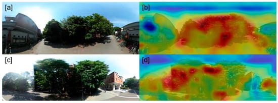
Figure 10.
The class activation map of the binary classification of tree and non-tree images with ResNet-50. The panels (a) and (c) show the original image of the 360° spherical camera. The panels (b) and (d) illustrate the class activation map. The maps were created based on [51]. The red and blue colors indicate the higher and lower activation, respectively.
3.2.2. Tree Detection from 360° Spherical Images Using YOLO v2
As shown in Figure 3b, the pre-trained networks, ResNet-50 and 4-layer CNN, were used for the feature extractor. In addition, the weights and biases were tuned with tree and non-tree image classification, as represented in Figure 6. The two feature extractors, which are original, and are tuned based on ResNet-50 and 4-layer CNN, was used for YOLO v2. Table 3 shows the average precision [52], which indicates the accuracy of the YOLO v2 detector. In Table 3, the result of YOLO v2 detector, which used pre-training for tuning the weights and bias in ResNet-50 and 4-layer CNN, as shown in the Section 3.2.1, is indicated as “Pre-training.” In contrast, the result when pre-training was not conducted is shown as “No pre-training.” There were no considerable differences between the “Pre-training” and the “No pre-training” results. The approximate model size of the YOLO v2 detector using ResNet-50 and the 4-layer CNN is also shown. This model size was based on results obtained using MATLAB software. The time for inference per image using the YOLO v2 detector with ResNet-50 and 4-layer CNN was 0.26 and 0.075 s, respectively.
Table 3.
Average precision of tree detection by the YOLO v2 detector. The feature extractor in the network was based on ResNet-50 and 4-layer CNN, as explained in the Section 2.5.2. The weight and bias were tuned for tree/non-tree classification, as shown in Section 3.2.1. The result with the network is denoted as “Pre-training”. In contrast, the result with no training, where the transferred ResNet-50 and 4-layer CNN with a randomly determined initial value were used, is represented by “No pre-training”. The approximate model size of the YOLO v2 detector using ResNet-50 and the 4-layer network in MATLAB is shown.
3.2.3. Tree Detection from the 3D Images Constructed by SfM
Figure 11 shows the tree detection result in the 3D images recovered by SfM. The panels [a] and [b] show the 3D images constructed by SfM. The 3D images were identical, but viewed from different angles. The 3D structure of plants could be reconstructed clearly, including color information and the shadow of the trees. Panel [c] represents the 3D image with the label “tree”. The blue points correspond to the tree detected using the YOLO v2 detector. Panel [d] shows the tree detection result. Each color represents different trees. The neighboring trees were illustrated with different colors. This implies that tree detection and classification could be carried out accurately. A different color, however, does not represent a different species. The trees are of the same species, namely ginkgo. As for the tree detection accuracy, the precision and recall were 0.88 and 1.0, respectively, and the F-measure was 0.94.
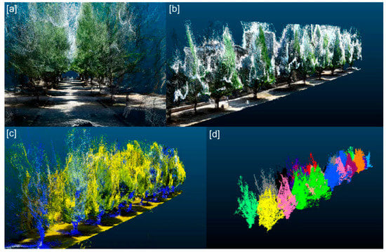
Figure 11.
Result of tree detection in 3D images reconstructed by SfM (structure from motion). Panels (a) and (b) represent 3D images constructed from a 360° spherical camera. Panel (c) illustrates the 3D image containing tree information obtained by YOLO v2 detector. The points corresponding to trees are indicated in blue. This 3D image underwent post-processing, and each tree could be segmented, as shown in panel (d). Each tree is illustrated by a different color.
4. Discussion
4.1. Tree Trunk Diameter and Height Estimation
Tree trunk diameter estimation could be carried out. According to Barazzetti et al [53], the accuracy of the 3D images reconstructed from spherical images was consistent with the typical results of more traditional photogrammetric projects based on central perspectives. The tree diameter estimation error was smaller when the video resolution was higher. 3D images from lower resolution videos contained missing points, and the points corresponding to the tree trunk could not be accurately reconstructed. This resulted in an estimation error of trunk diameters. The higher resolution leads to an increase in the correct image matching in the process of SfM. When the distance to the target is 4 m, the tree trunk estimation error was lower than when the target was 8 m away, with an image resolution of 3840×1920. This is because the point matching among input images was successfully conducted when the distance from the target is shorter, resulting in more detailed 3D reconstruction. A higher resolution and shorter distances between the target and the camera are desirable in terms of accuracy. However, a higher resolution leads to longer processing times for 3D reconstruction. Therefore, appropriate conditions should be determined based on experiments.
Tree height estimation was not considerably dependent on the tree height of the target tree. However, the tree top could not be reconstructed when conducting measurements beneath the canopy. If the canopy blocks the line of sight to the tree top, and it cannot be observed by the camera, the tree height is underestimated. It is not rare that approximating height suffices, and more precise values are typically not required. An example of this is a forest investigation. In such cases, the tree height under tree canopies is estimated, even with an approximate accuracy would be useful.
Videos were recorded while walking to acquire numerous images with a high overlap ratio. When the movement speed is higher, blurred images will be included in the frames, preventing the model from constructing 3D images.
However, these blurred images can be excluded using deep learning [54], allowing large-area measurement with a higher moving speed. As shown in Figure 11a,b, the color information was also recovered. Chlorophyll distribution in small plants could be estimated accurately using SfM [55]. Additionally, a previous study reported a method which combines the 3D point clouds derived from LiDAR, and multi-spectral images for estimating the chlorophyll distribution of a bigger tree [56]. Depending on the foliage structure, a serious occlusion of the inner crown is shown, however, it can be alleviated when the spherical camera is used for the image acquisition while moving, and the 3D information is reconstructed using structure from the motion algorithm. The chlorophyll distribution in trees could also be estimated.
4.2. Automatic Tree Detection
As shown in Table 3, accurate tree detection from 360° spherical images could be accomplished with the YOLO v2 detector. The image dataset was obtained from video frames in this study. Images obtained from a series of video frames were divided into training and test images, so that, sometimes, images can be similar to each other. This would increase the average precision of detection. Then, the average precision, as shown in Table 3, may not be equivalent to an accuracy with the unknown images. However, accurate tree detection was confirmed, even with other images that were not included in the training or test datasets like the images used for the 3D reconstruction and the tree detection in the 3D space. In addition, the highlight of this study was the accuracy of tree detection from 3D images reconstructed using SfM, and not the average precision of the YOLO detector itself. Trees have complicated shapes, which are difficult to be defined quantitatively. Accordingly, it is difficult to detect them with rule-based image processing techniques. In contrast, a deep learning-based approach for object detection such as YOLO does not require defining features. In terms of including unnecessary definitions of tree features, using the YOLO network is effective. Here, a good performance of the tree detection from the spherical images was observed. However, if higher performance is required, other pre-trained networks that accept the larger size of the images can be tested.
The images included in the dataset, ImageNet and the tree are not very similar. Therefore, the weight and bias values in ResNet-50 may be inappropriate for the feature extractor of tree images. As the activation map in Figure 10 shows, the network extracts the appropriate features of trees, which increases the reliability of the feature extractor itself. Furthermore, if the accuracy of the binary classification is sufficient, but the activation locates a region which is not related to the region of interest, the network is implied to be inappropriate for the feature extractor. This kind of confirmation could make the detection system robust and reliable. Although there are no significant differences between the results obtained with and without pre-training, pre-training could increase the object detection accuracy in other tasks. This pre-training does not require annotation for rectangle labeling of the targets, just because the training is for classification. While the object detection necessitates the labeling of all objects of interest, the classification does not need it, leading to ease in the collection of training and test images.
High average precision could also be obtained with the 4-layer CNN for the feature extractor. In this study, the detection targets were only trees, leading to a high detection accuracy with the simple CNN architecture as a feature extractor. The model size of the YOLO v2 detector with the 4-layer CNN was much smaller than that with ResNet-50, as shown in Table 3, which is convenient for its implementation. Moreover, the smaller number of parameters enables faster inference and the careful adjustment of hyper-parameters in training due to shorter training times. Therefore, a pre-trained network was not necessarily required as a feature extractor, especially when the target to detect did not vary widely.
The accuracy with “No pre-training” was also sufficiently high for tree detection. The features obtained via the convolutional operations of pre-trained networks are called Deep Convolutional Activation Feature (Decaf), and it returns the features that are effective for object recognition [57].
We wanted the weights and biases in ResNet-50 and the 4-layer CNN to be optimized via the pre-training, as shown in Figure 6. However, it can be suggested that the features that should be returned could be sufficiently acquired from the training process in YOLO v2, without pre-training. Furthermore, as for ResNet-50, the network was trained with ImageNet, which includes a wide variety of general images. The 360° spherical images were taken outdoors. ImageNet comprises several natural scenes as well. The similarity of those images could contribute to the accuracy of the YOLO v2 detector without pre-training. The pre-training of the feature extractor could contribute to higher accuracy when the images in ImageNet and the targets in the new task are completely different. The necessity and effectiveness this feature extractor’s pre-training will be dependent on the tasks and the network. Tree detection using YOLO v2 was performed on the 3D images reconstructed using SfM in this study. However, tree detection in the 2D images itself will be useful for purposes with 2D-based tasks. For example, a map with tree species in a target area could be made by combining this tree identification method and tree species classification.
4.3. Tree Detection in 3D Images
Tree detection from the 3D images could be done with a high F-measure of 0.94. This is due to the fact that the 2D images were taken by 360° spherical cameras. After 3D reconstruction, the regions corresponding to the tree trunk and the lower part of the tree canopy were clustered, as shown in Figure 9c. If the number of points constituting the region was less than 100, the region was deleted, because it was recognized as a noise cluster. However, if the tree trunk diameter is small, it will also be deleted due to the small number of points, resulting in an omission error. Moreover, if the tree trunk diameter is very small, that part is difficult to be recovered into 3D images using SfM; this can also result in an omission error. However, there were no omission errors in this study. The accurate YOLO v2 detector detected the trees, and only a few non-tree objects were recognized as trees. This automatic tree detection leads to automated tree structural parameters extraction. The tree trunk can be calculated using a circle or a cylinder fitting, and the tree height can also be estimated. Therefore, it was suggested that after image acquisition, all processes from tree detection to structural parameter retrieval can be done automatically, which can contribute to many fields, such as labor-less forest research and tree administration in urban streets and parks.
4.4. Comparison with the Automatic Tree Detection from LiDAR 3D Images
Some previous studies utilized 3D image processing for tree detection from LiDAR 3D images. For example, a cylinder or circle was fitted to tree trunks [23,24]. Other methods that combine 3D image processing and machine leaning techniques have also been reported [48]. The study, first, detected tree trunks and excluded non-tree objects, using a one-class support vector machine. However, the tree trunks in the LiDAR 3D images were not as clear as the ones in 2D images, causing their omission. Furthermore, artificial objects with pole-like structures are mis-recognized as trees, especially with a cylinder or circle fitting. In contrast, the 2D images capture tree shapes with a high resolution and color information as shown in this study, enabling accurate tree detection, even with complicated backgrounds. One advantage of the use of 2D image is the high resolution, which may make it possible to classify the tree species through the information of the 2D images. Species classification with 3D point clouds is not easy. Further, more object detection algorithms are available for 2D images than for 3D point clouds. We employed a deep learning-based method (YOLO v2) for tree detection, which can be used with other non-tree objects in the background. With this method, a high detection performance could be observed. On the other hand, if we would like a deep neural network to train with 3D input data, the time for training and inference would be longer, and to collect the training data is not easy. As the laser beam emitted from LiDAR is invisible in many cases, it becomes difficult to check if the laser beam successfully reaches the target. If the target is not emitted by the laser beam, the target cannot be reconstructed into 3D images. On the other hand, the measurement with the 360° spherical camera can be done with portable devices, such as smart phones. This allowed for the entire area for taking measurements to be checked.
If the camera position or angle is not appropriate, it is comparatively easy to fix them when measuring the study sites with the 360° spherical camera. To our best knowledge, few studies have showed the feasibility of plant measurements with the 360° spherical camera and 3D reconstruction, using SfM. The result from the omnidirectional image acquisition to the automatic object identification in a 3D space would be valuable.
5. Conclusions
In this study, the feasibility of a 360° spherical camera was examined, and a method for the automatic detection of trees in 3D images, reconstructed using SfM, was demonstrated. First, the tree trunk diameter and its height were estimated from the 3D images reconstructed from the 360° images. The images of trees were taken using a 360° spherical camera of THETA V and THETA SC. Then, the 3D images were reconstructed using SfM. From the 3D images, the tree trunk diameter and height were estimated, and these values were compared with their measured values. As a result, the tree trunk diameter could be estimated with an absolute error of less than 3 cm. The tree height estimation error was approximately 50 cm. We found that the tree trunk diameter and height can be estimated by combining a 360° spherical camera and the photometric approach, SfM. When the resolution of the spherical images was higher, the 3D images have fewer missing points, resulting in a higher estimation accuracy. When we use a LiDAR for the tree trunk diameter estimation, the accuracy would be higher than one with the spherical camera in this study. However, the diameter estimation result with the spherical camera could be enhanced, for example, by increasing the number of input or optimizing the angle and distance to the target from the camera. In our future work, we try to improve the diameter estimation accuracy more.
Next, a method for detecting trees in the 3D images, constructed using SfM, was proposed. First, the trees in the 360° spherical images were detected using a deep learning-based detector, YOLO v2. For the YOLO v2 detector, a pre-trained network, ResNet-50, or convolutional neural network with four layers (4-layer CNN) was used. The weights and biases in ResNet-50 and 4-layer CNN were changed via the binary classification of tree and non-tree objects. Instead of using the weight and bias value of ResNet-50 or randomly determined values in a 4-layer CNN, the adjusted values for the tree/non-tree classification were used. The class activation map for classifying an image shows that the branch-like objects were considered, and the images were classified into trees. This implies that the network is appropriate for extracting tree features. The result of tree detection using the YOLO v2 detector with the network indicated higher detection accuracy. In the tree detection from 3D images, the trees could be accurately detected with an F-measure value of 0.94. We found that the trees in the 3D images can be detected using the tree detection in the 2D images. Accurate tree detection using YOLO v2 leads to a higher detection accuracy. The tree detection from 360° spherical images was demonstrated accurately with a 4-layer CNN, with model size considerably smaller than that of ResNet-50. It contributes to a shorter training time, inference time and ease of tuning the hyper-parameters in training.
This study reveals the feasibility of the combination of 360° spherical cameras, automatic object detection and 3D reconstruction, using SfM. This technique can not only help in tree structural parameter extraction, as in this study, but could also be a solution for a wide variety of plant measurements. For example, plant disease detection will be possible by detecting leaves and classifying its condition. The structural information can be obtained with 3D reconstruction. In the discussion section, the use of LiDAR and that of the 360° spherical camera were compared. However, it is possible to combine them. An example of this is a sensor fusion technique. A technique which combines LiDAR 3D imaging and multi-spectral imaging has been reported [56]. It may be possible to automatically project the 360° image onto the LiDAR 3D image to retrieve physiological parameters from the detailed LiDAR 3D image and the spectral information. In our future work, other structural parameters, such as crown diameter, branch patterns and the branch angles, will be calculated, and the tree identification method should be tested with much more images. In addition, the parameters estimated in this study (i.e., tree trunk diameter and height) should be estimated automatically after the automatic tree separation in the 3D images.
Author Contributions
K.I. conducted the experiment and analysis. This paper was written by K.I. with the supervision of F.H. All authors have read and agreed to the published version of the manuscript.
Funding
This work was supported by JSPS KAKENHI Grant Number JP19J22701.
Conflicts of Interest
The authors declare no conflict of interest.
References
- Miller, J.; Morgenroth, J.; Gomez, C. 3D modelling of individual trees using a handheld camera: Accuracy of height, diameter and volume estimates. Urban Fore. Urban Green. 2015, 14, 932–940. [Google Scholar] [CrossRef]
- Oshio, H.; Asawa, T.; Hoyano, A.; Miyasaka, S. Estimation of the leaf area density distribution of individual trees using high-resolution and multi-return airborne LiDAR data. Remote Sens. Environ. 2015, 166, 116–125. [Google Scholar] [CrossRef]
- Chen, C.; Wang, Y.; Li, Y.; Yue, T.; Wang, X. Robust and Parameter-Free Algorithm for Constructing Pit-Free Canopy Height Models. ISPRS Int. J. Geo-Info. 2017, 6, 219. [Google Scholar] [CrossRef]
- Nelson, R.; Krabill, W.; Tonelli, J. Estimating forest biomass and volume using airborne laser data. Remote sensing of environment. Remote Sens. Environ. 1988, 24, 247–267. [Google Scholar] [CrossRef]
- Omasa, K.; Hosoi, F.; Konishi, A. 3D lidar imaging for detecting and understanding plant responses and canopy structure. Exp. Bot. 2007, 58, 881–898. [Google Scholar] [CrossRef]
- Hosoi, F.; Omasa, K. Voxel-based 3-D modeling of individual trees for estimating leaf area density using high-resolution portable scanning lidar. IEEE Trans. Geosci. Remote. 2006, 44, 3610–3618. [Google Scholar] [CrossRef]
- Hosoi, F.; Omasa, K. Factors contributing to accuracy in the estimation of the woody canopy leaf-area-density profile using 3D portable lidar imaging. J. Exp. Bot. 2007, 58, 3464–3473. [Google Scholar] [CrossRef]
- Hosoi, F.; Nakai, Y.; Omasa, K. 3-D voxel-based solid modeling of a broad-leaved tree for accurate volume estimation using portable scanning lidar. ISPRS J. Photogramm. 2013, 82, 41–48. [Google Scholar] [CrossRef]
- Bailey, B.N.; Mahaffee, W.F. Rapid measurement of the three-dimensional distribution of leaf orientation and the leaf angle probability density function using terrestrial LiDAR scanning. Remote Sens. Environ. 2017, 194, 63–76. [Google Scholar] [CrossRef]
- Itakura, K.; Hosoi, F. Estimation of Leaf Inclination Angle in Three-Dimensional Plant Images Obtained from Lidar. Remote Sens. 2019, 11, 344. [Google Scholar] [CrossRef]
- Pan, Y.; Kuo, K.; Hosoi, F. A study on estimation of tree trunk diameters and heights from three-dimensional point cloud images obtained by SLAM. Eco Eng. 2017, 29, 17–22. [Google Scholar]
- Jozkow, G.; Totha, C.; Grejner-Brzezinska, D. UAS topographic mapping with velodyne lidar sensor. ISPRS Ann. Photogram. Remote Sens. Spatial Info. Sci. 2016, 3, 201–208. [Google Scholar] [CrossRef]
- Elaksher, A.F.; Bhandari, S.; Carreon-Limones, C.A.; Lauf, R. Potential of UAV lidar systems for geospatial mapping. In Lidar Remote Sensing for Environmental Monitoring 2017. Int. Soc. Opt. Photon. 2017, 10406, 104060L. [Google Scholar]
- Liu, K.; Shen, X.; Cao, L.; Wang, G.; Cao, F. Estimating forest structural attributes using UAV-LiDAR data in Ginkgo plantations. ISPRS J. Photogram. Remote Sens. 2018, 146, 465–482. [Google Scholar] [CrossRef]
- Westoby, M.J.; Brasington, J.; Glasser, N.F.; Hambrey, M.J.; Reynolds, J.M. ‘Structure-from-Motion’photogrammetry: A low-cost, effective tool for geoscience applications. Geomorphology 2012, 179, 300–314. [Google Scholar] [CrossRef]
- Liang, X.; Jaakkola, A.; Wang, Y.; Hyyppä, J.; Honkavaara, E.; Liu, J.; Kaartinen, H. The use of a hand-held camera for individual tree 3D mapping in forest sample plots. Remote Sens. 2014, 6, 6587–6603. [Google Scholar] [CrossRef]
- Piermattei, L.; Karel, W.; Wang, D.; Wieser, M.; Mokroš, M.; Surový, P.; Koreň, M.; Tomaštík, J.; Pfeifer, N.; Hollaus, M. Terrestrial Structure from Motion Photogrammetry for Deriving Forest Inventory Data. Remote Sens. 2019, 11, 950. [Google Scholar] [CrossRef]
- Qiu, Z.; Feng, Z.; Jiang, J.; Lin, Y.; Xue, S. Application of a continuous terrestrial photogrammetric measurement system for plot monitoring in the Beijing Songshan national nature reserve. Remote Sens. 2018, 10, 1080. [Google Scholar] [CrossRef]
- Itakura, K.; Kamakura, I.; Hosoi, F. A Comparison study on three-dimensional measurement of vegetation using lidar and SfM on the ground. Eco Eng. 2018, 30, 15–20. [Google Scholar]
- Barazzetti, L.; Previtali, M.; Roncoroni, F. 3D modelling with the Samsung Gear 360. In Proceedings of the 2017 TC II and CIPA-3D Virtual Reconstruction and Visualization of Complex Architectures, International Society for Photogrammetry and Remote Sensing, Nafplio, Greece, 1–3 March 2017. [Google Scholar]
- Firdaus, M.I.; Rau, J.-Y. Accuracy analysis of three-dimensional model reconstructed by spherical video images. In Proceedings of the International Symposium on Remote Sensing (ISPRS 2018), Dehradun, India, 20–23 November 2018. [Google Scholar]
- Honjo, T.; Lin, T.-P.; Seo, Y. Sky view factor measurement by using a spherical camera. J. Agric. Meteol. 2019, 75, 59–66. [Google Scholar] [CrossRef]
- Aschoff, T.; Spiecker, H. Algorithms for the automatic detection of trees in laser scanner data. Proceedings of International Archives of Photogrammetry, Remote Sensing and Spatial Information Sciences 2004. Available online: https://www.isprs.org/proceedings/xxxvi/8-w2/aschoff.pdf (accessed on 25 October 2019).
- Henning, J.G.; Radtke, P.J. Detailed stem measurements of standing trees from ground-based scanning lidar. Forest Sci. 2006, 52, 67–80. [Google Scholar]
- Lovell, J.L.; Jupp, D.L.B.; Newnham, G.J.; Culvenor, D.S. Measuring tree stem diameters using intensity profiles from ground-based scanning lidar from a fixed viewpoint. ISPRS J. Photogram. Remote Sens. 2011, 66, 46–55. [Google Scholar] [CrossRef]
- Liang, X.; Hyyppä, J.; Kaartinen, H.; Wang, Y. International benchmarking of terrestrial laser scanning approaches for forest inventories. ISPRS J. Photogram. Remote Sens. 2018, 144, 137–179. [Google Scholar] [CrossRef]
- Girshick, R.; Donahue, J.; Darrell, T.; Malik, J. Rich feature hierarchies for accurate object detection and semantic segmentation. In Proceedings of the 27th IEEE conference on computer vision and pattern recognition, Columbus, OH, USA, 24–27 June 2014. [Google Scholar]
- A Zhang, T.; Zhang, X. High-Speed Ship Detection in SAR Images Based on a Grid Convolutional Neural Network. Remote Sens. 2019, 11, 1206. [Google Scholar] [CrossRef]
- Girshick, R. Fast r-cnn. In Proceedings of the 28th IEEE conference on computer vision and pattern recognition, Boston, MA, USA, 7–12 June 2015. [Google Scholar]
- Ren, S.; He, K.; Girshick, R.; Sun, J. Faster r-cnn: Towards real-time object detection with region proposal networks. In Proceedings of the 29th Conference on Neural Information Processing Systems, Montreal, QC, Canada, 7–12 December 2015. [Google Scholar]
- Redmon, J.; Divvala, S.; Girshick, R.; Farhadi, A. You only look once: Unified, real-time object detection. In Proceedings of the 29th IEEE Conference on Computer Vision and Pattern Recognition, Las Vegas, NV, USA, 26 June–1 July 2016. [Google Scholar]
- Liu, W.; Anguelov, D.; Erhan, D.; Szegedy, C.; Reed, S.; Fu, C.-Y.; Berg, A.C. Ssd: Single shot multibox detector. In Proceedings of the 14th European Conference on Computer Vision, Amsterdam, The Netherlands, 8–16 October 2016. [Google Scholar]
- Redmon, J.; Farhadi, A. YOLO9000: better, faster, stronger. In Proceedings of the 30th IEEE Conference on Computer Vision and Pattern Recognition, Honolulu, HI, USA, 22–25 July 2017. [Google Scholar]
- Zhang, J.; Singh, S. 2014: LOAM: Lidar odometry and mapping in real-time. In Proceedings of the Robotics: Science and Systems Conference (RSS), Berkeley, CA, USA, 12–16 July 2014. [Google Scholar]
- RICHO THETA ACCESORY. Available online: https://theta360.com/en/ (accessed on 25 October 2019).
- RICHO THETA ACCESORY. Available online: https://theta360.com/en/about/theta/accessory.html (accessed on 25 October 2019).
- Verhoeven, G. Taking computer vision aloft–archaeological three-dimensional reconstructions from aerial photographs with photoscan. Archaeol. Prospect. 2011, 18, 67–73. [Google Scholar] [CrossRef]
- Neubeck, A.; Van Gool, L. Efficient non-maximum suppression. In Proceedings of the 18th International Conference on Pattern Recognition, Hong Kong, China, 20–24 August 2006. [Google Scholar]
- He, K.; Zhang, X.; Ren, S.; Sun, J. Deep residual learning for image recognition. In Proceedings of the 29th IEEE Conference on Computer Vision and Pattern Recognition, Las Vegas, NV, USA, 26 June–1 July 2016. [Google Scholar]
- Deng, J.; Dong, W.; Socher, R.; Li, L.J.; Li, K.; Fei-Fei, L. Imagenet: A large-scale hierarchical image database. In Proceedings of the IEEE Conference on Computer Vision and Pattern Recognition, Miami, FL, USA, 20–25 June 2009. [Google Scholar]
- Szegedy, C.; Liu, W.; Jia, Y.; Sermanet, P.; Reed, S.; Anguelov, D.; Erhan, D.; Vanhoucke, V.; Rabinovich, A. Going deeper with convolutions. In Proceedings of the 28th IEEE conference on computer vision and pattern recognition, Boston, MA, USA, 7–12 June 2015. [Google Scholar]
- Glorot, X.; Bengio, Y. Understanding the difficulty of training deep feedforward neural networks. In Proceedings of the thirteenth international conference on artificial intelligence and statistics, Sardinia, Italy, 13–15 May 2010. [Google Scholar]
- Mathworks Documentation, trainYOLOv2ObjectDetector, training Loss. Available online: https://jp.mathworks.com/help/vision/ref/trainyolov2objectdetector.html (accessed on 25 October 2019).
- Goodfellow, I.; Bengio, Y.; Courville, A. Deep learning; MIT press Cambridge: London, UK, 2016. [Google Scholar]
- Mathworks Documentation, trainingOptions, ValidationPatience. Available online: https://jp.mathworks.com/help/deeplearning/ref/trainingoptions.html?lang=en (accessed on 25 October 2019).
- Park, H.-S.; Jun, C.-H. A simple and fast algorithm for K-medoids clustering. Expert Syst. Appl. 2009, 36, 3336–3341. [Google Scholar] [CrossRef]
- Itakura, K.; Hosoi, F. Automatic individual tree detection and canopy segmentation from three-dimensional point cloud images obtained from ground-based lidar. J. Agric. Meteol. 2018, 74, 109–113. [Google Scholar] [CrossRef]
- Itakura, K.; Hosoi, F. Automated tree detection from 3D lidar images using image processing and machine learning. Appl. Opt. 2019, 58, 3807–3811. [Google Scholar] [CrossRef]
- Torr, P.H.S.; Zisserman, A. MLESAC: A new robust estimator with application to estimating image geometry. Comput. Vis. Image Und. 2000, 78, 138–156. [Google Scholar] [CrossRef]
- Rusu, R.B.; Marton, Z.C.; Blodow, N.; Dolha, M.; Beetz, M. Towards 3D point cloud based object maps for household environments. Robot. Auton. Syst. 2008, 56, 927–941. [Google Scholar] [CrossRef]
- Zhou, B.; Khosla, A.; Lapedriza, A.; Oliva, A.; Torralba, A. Learning deep features for discriminative localization. In Proceedings of the 29th IEEE Conference on Computer Vision and Pattern Recognition, Las Vegas, NV, USA, 26 June–1 July 2016. [Google Scholar]
- Henderson, P.; Ferrari, V. End-to-end training of object class detectors for mean average precision. In Proceedings of the 13th Asian Conference on Computer Vision, Taipei, Taiwan, 20–24 November 2016. [Google Scholar]
- Barazzetti, L.; Previtali, M.; Roncoroni, F. Can we use low-cost 360 degree cameras to create accurate 3D models? In Proceedings of the ISPRS TC II Mid-term Symposium “Towards Photogrammetry 2020”, Riva del Garda, Italy, 4–7 June 2018. [Google Scholar]
- Itakura, K.; Hosoi, F. Estimation of tree structural parameters from video frames with removal of blurred images using machine learning. J. Agric. Meteol. 2018, 74, 154–161. [Google Scholar] [CrossRef]
- Itakura, K.; Kamakura, I.; Hosoi, F. Three-Dimensional Monitoring of Plant Structural Parameters and Chlorophyll Distribution. Sensors 2019, 19, 413. [Google Scholar] [CrossRef] [PubMed]
- Hosoi, F.; Umeyama, S.; Kuo, K. Estimating 3D chlorophyll content distribution of trees using an image fusion method between 2D camera and 3D portable scanning lidar. Remote Sens. 2019, 11, 2134. [Google Scholar] [CrossRef]
- Donahue, J.; Jia, Y.; Vinyals, O.; Hoffman, J.; Zhang, N.; Tzeng, E.; Darrell, T. Decaf: A deep convolutional activation feature for generic visual recognition. Proc. Int. Conf. Mach. Learn. 2014, 647–655. [Google Scholar]


© 2020 by the authors. Licensee MDPI, Basel, Switzerland. This article is an open access article distributed under the terms and conditions of the Creative Commons Attribution (CC BY) license (http://creativecommons.org/licenses/by/4.0/).