OIC-MCE: A Practical Land Cover Mapping Approach for Limited Samples Based on Multiple Classifier Ensemble and Iterative Classification

 , ,
, ,
Abstract

1. Introduction
2. Study Area and Data
2.1. Study Area
2.2. Data
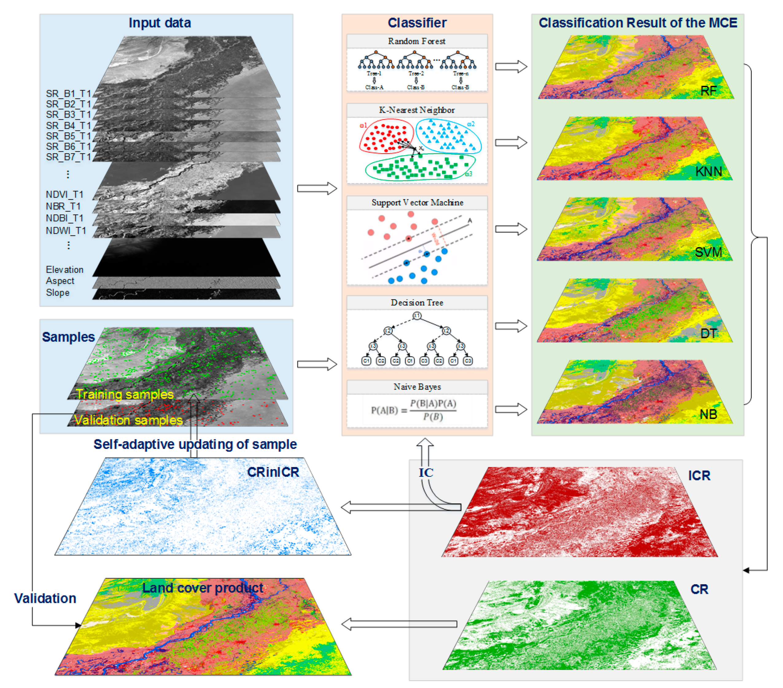
3. Methodology
3.1. Initial Training Samples Collection
3.2. Object-Oriented Multi-Resolution Segmentation and Classification Features Selection
3.3. Multiple Classifiers Ensemble (MCE)
3.4. Self-Adaptive Updating of Training Samples
3.5. Iterative Classification (IC)
3.6. Integration of Iterative Classification Result
3.7. Accuracy Assessment
4. Results
4.1. The Self-Adaptively Updated Training Samples
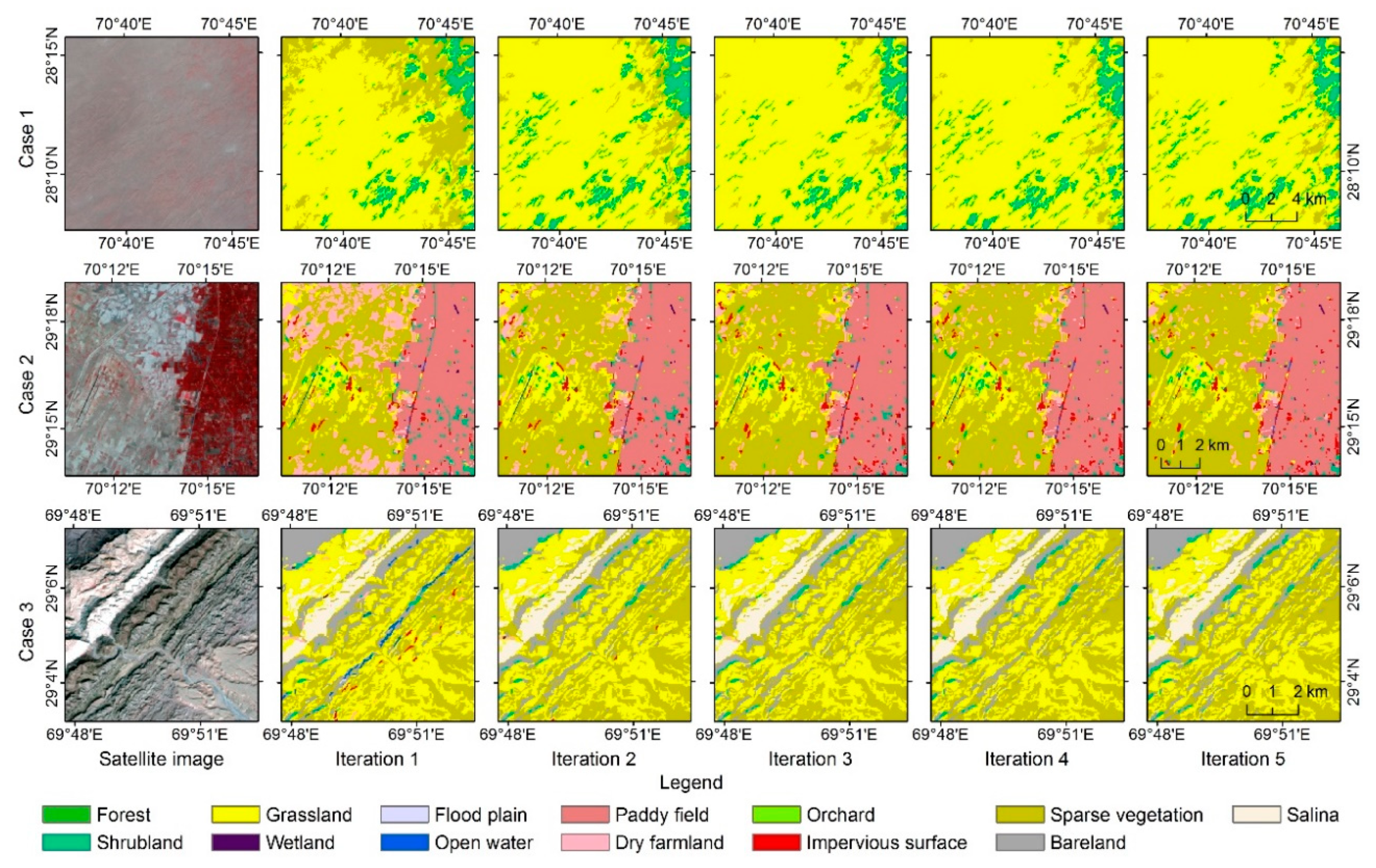
4.2. The CR of Each Iteration
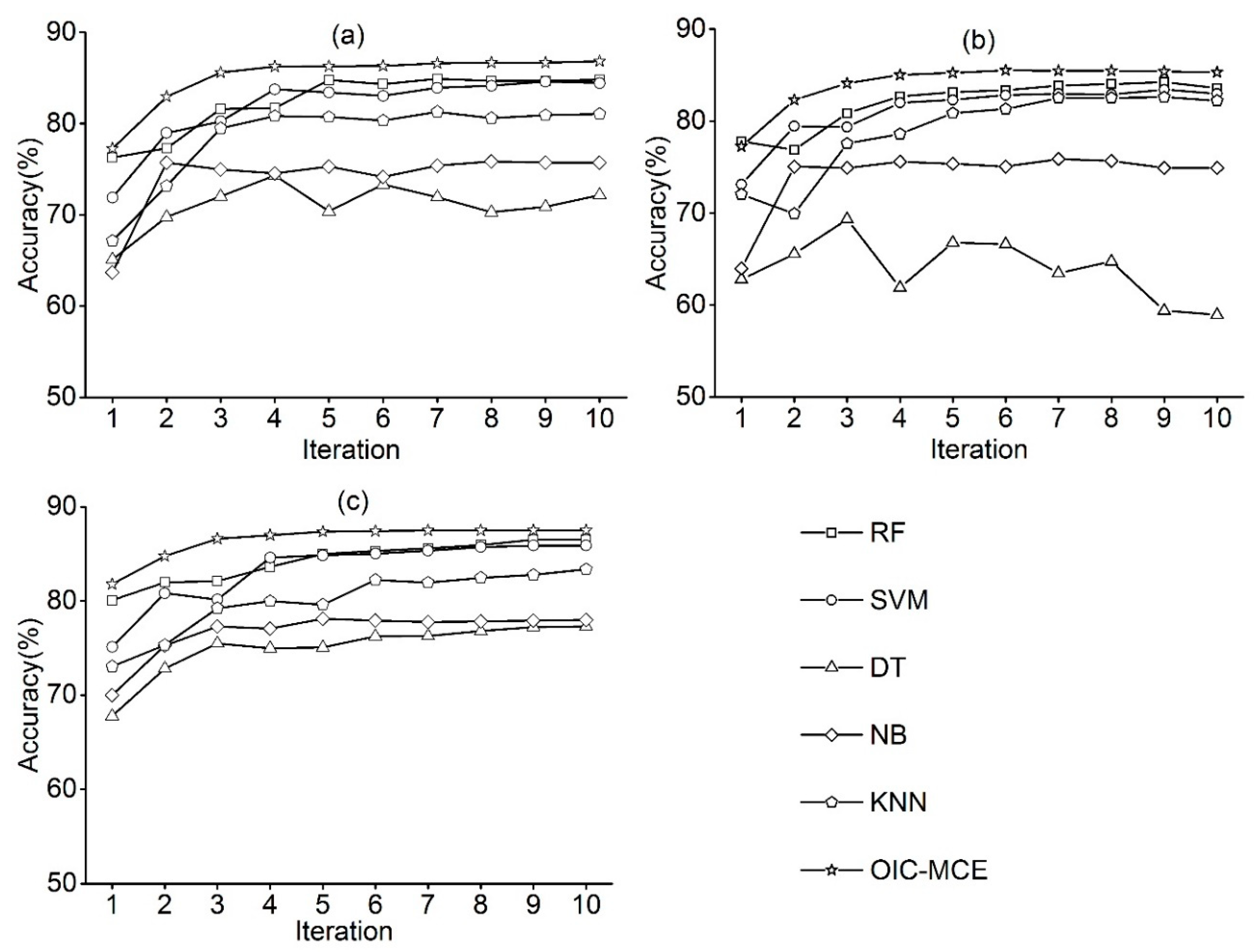
4.3. The Accuracy of the OIC-MCE and Each Single Classifier in the Iterative Process
4.4. The Accuracy of Each Land Cover Class in Iterative Classification
5. Discussion
5.1. Adaptively Updating of Training Samples
5.2. The OIC-MCE
5.2.1. Effects of Initial Sample Size on the Performance of the OIC-MCE Method
5.2.2. The Stability of the OIC-MCE Method
5.3. Merits and Limitations of the Proposed Method
5.4. Application of the Proposed OIC-MCE Method in the Land Cover Mapping of CPEC
6. Conclusions
Supplementary Materials
Author Contributions
Funding
Acknowledgments
Conflicts of Interest
References
- Wulder, M.A.; Coops, N.C.; Roy, D.P.; White, J.C.; Hermosilla, T. Land cover 2.0. Int. J. Remote Sens. 2018, 39, 4254–4284. [Google Scholar] [CrossRef]
- Turner, B.L.; Lambin, E.F.; Reenberg, A. The emergence of land change science for global environmental change and sustainability. Proc. Natl. Acad. Sci. USA 2007, 104, 20666–20671. [Google Scholar] [CrossRef] [PubMed]
- Gómez, C.; White, J.C.; Wulder, M.A. Optical remotely sensed time series data for land cover classification: A review. ISPRS J. Photogramm. Remote Sens. 2016, 116, 55–72. [Google Scholar] [CrossRef]
- Phiri, D.; Morgenroth, J. Developments in landsat land cover classification methods: A review. Remote Sens. 2017, 9, 967. [Google Scholar] [CrossRef]
- Gong, P.; Yu, L.; Li, C.; Wang, J.; Liang, L.; Li, X.; Ji, L.; Bai, Y.; Cheng, Y.; Zhu, Z. A new research paradigm for global land cover mapping. Ann. GIS 2016, 22, 87102. [Google Scholar] [CrossRef]
- Pandey, P.C.; Koutsias, N.; Petropoulos, G.P.; Srivastava, P.K.; Ben Dor, E. Land use/land cover in view of earth observation: Data sources, input dimensions, and classifiers-a review of the state of the art. Geocarto Int. 2019, 191, 1–32. [Google Scholar] [CrossRef]
- Ma, L.; Li, M.; Ma, X.; Cheng, L.; Du, P.; Liu, Y. A review of supervised object-based land-cover image classification. ISPRS J. Photogramm. Remote Sens. 2017, 130, 277293. [Google Scholar] [CrossRef]
- Yang, L.; Jin, S.; Danielson, P.; Homer, C.; Gass, L.; Bender, S.M.; Case, A.; Costello, C.; Dewitz, J.; Fry, J.; et al. A new generation of the United States National Land Cover Database: Requirements, research priorities, design, and implementation strategies. ISPRS J. Photogramm. Remote Sens. 2018, 146, 108123. [Google Scholar] [CrossRef]
- Li, C.; Gong, P.; Wang, J.; Zhu, Z.; Biging, G.S.; Yuan, C.; Hu, T.; Zhang, H.; Wang, Q.; Li, X.; et al. The first all-season sample set for mapping global land cover with Landsat-8 data. Sci. Bull. 2017, 62, 508–515. [Google Scholar] [CrossRef]
- Zhao, Y.Y.; Gong, P.; Yu, L.; Hu, L.Y.; Li, X.Y.; Li, C.C.; Zhang, H.Y.; Zheng, Y.M.; Wang, J.; Zhao, Y.C.; et al. Towards a common validation sample set for global land-cover mapping. Int. J. Remote Sens. 2014, 35, 4795–4814. [Google Scholar] [CrossRef]
- Stehman, S.V. Sampling designs for accuracy assessment of land cover. Int. J. Remote Sens. 2009, 30, 5243–5272. [Google Scholar] [CrossRef]
- Xie, H.; Li, A.; Tang, J.; Lei, G.; Bian, J. Research and application on the field sampling software of the land use and land cover in the mountainous area. Remote Sens. Technol. Appl. 2016, 31, 430–437. [Google Scholar] [CrossRef]
- Fritz, S.; McCallum, I.; Schill, C.; Perger, C.; See, L.; Schepaschenko, D.; van der Velde, M.; Kraxner, F.; Obersteiner, M. Geo-Wiki: An online platform for improving global land cover. Environ. Modell. Softw. 2012, 31, 110–123. [Google Scholar] [CrossRef]
- Stehman, S.V.; Fonte, C.C.; Foody, G.M.; See, L. Using volunteered geographic information (VGI) in design-based statistical inference for area estimation and accuracy assessment of land cover. Remote Sens. Environ. 2018, 212, 47–59. [Google Scholar] [CrossRef]
- Gong, P.; Liu, H.; Zhang, M.; Li, C.; Wang, J.; Huang, H.; Clinton, N.; Ji, L.; Li, W.; Bai, Y.; et al. Stable classification with limited sample: Transferring a 30-m resolution sample set collected in 2015 to mapping 10-m resolution global land cover in 2017. Sci. Bull. 2019, 64, 370–373. [Google Scholar] [CrossRef]
- Mountrakis, G.; Im, J.; Ogole, C. Support vector machines in remote sensing: A review. ISPRS J. Photogramm. Remote Sens. 2011, 66, 247–259. [Google Scholar] [CrossRef]
- Belgiu, M.; Drăguţ, L. Random forest in remote sensing: A review of applications and future directions. ISPRS J. Photogramm. Remote Sens. 2016, 114, 24–31. [Google Scholar] [CrossRef]
- Li, A.; Jiang, J.; Bian, J.; Deng, W. Combining the matter element model with the associated function of probability transformation for multi-source remote sensing data classification in mountainous regions. ISPRS J. Photogramm. Remote Sens. 2012, 67, 80–92. [Google Scholar] [CrossRef]
- Wessel, M.; Brandmeier, M.; Tiede, D. Evaluation of Different Machine Learning Algorithms for Scalable Classification of Tree Types and Tree Species Based on Sentinel-2 Data. Remote Sens. 2018, 10, 1419. [Google Scholar] [CrossRef]
- Li, M.; Ma, L.; Blaschke, T.; Cheng, L.; Tiede, D. A systematic comparison of different object-based classification techniques using high spatial resolution imagery in agricultural environments. Int. J. Appl. Earth Obs. Geoinf. 2016, 49, 87–98. [Google Scholar] [CrossRef]
- Steele, B.M. Combining multiple classifiers: An application using spatial and remotely sensed information for land cover type mapping. Remote Sens. Environ. 2000, 74, 545–556. [Google Scholar] [CrossRef]
- Zhong, B.; Yang, A.X.; Nie, A.H.; Yao, Y.J.; Zhang, H.; Wu, S.L.; Liu, Q.H. Finer resolution land-cover mapping using multiple classifiers and multisource remotely sensed data in the heihe river basin. IEEE JSTARS 2015, 8, 4973–4992. [Google Scholar] [CrossRef]
- Shen, H.F.; Lin, Y.H.; Tian, Q.J.; Xu, K.J.; Jiao, J.N. A comparison of multiple classifier combinations using different voting-weights for remote sensing image classification. Int. J. Remote Sens. 2018, 39, 3705–3722. [Google Scholar] [CrossRef]
- Bian, Z.; Tang, P.; Yan, J. Land-cover classification from multiple classifiers using decision fusion based on the probabilistic graphical model. Int. J. Remote Sens. 2019, 40, 4560–4576. [Google Scholar] [CrossRef]
- Du, P.; Xia, J.; Zhang, W.; Tan, K.; Liu, Y.; Liu, S. Multiple classifier system for remote sensing image classification: A review. Sensors 2012, 12, 4764–4792. [Google Scholar] [CrossRef]
- Jia, K.; Li, Q.Z.; Wei, X.Q.; Zhang, L.; Du, X.; Yao, Y.J.; Wang, X.X. Multi-temporal remote sensing data applied in automatic land cover update using iterative training sample selection and Markov Random Field model. Geocarto Int. 2015, 30, 882–893. [Google Scholar] [CrossRef]
- Mack, B.; Roscher, R.; Stenzel, S.; Feilhauer, H.; Schmidtlein, S.; Waske, B. Mapping raised bogs with an iterative one-class classification approach. ISPRS J. Photogramm. Remote Sens. 2016, 120, 53–64. [Google Scholar] [CrossRef]
- Zhou, Z.H.; Li, M. Tri-training: Exploiting unlabeled data using three classifiers. IEEE Trans. Knowl. Data Eng. 2005, 17, 1529–1541. [Google Scholar] [CrossRef]
- Han, X.P.; Huang, X.; Li, J.Y.; Li, Y.S.; Yang, M.Y.; Gong, J.Y. The edge-preservation multi-classifier relearning framework for the classification of high-resolution remotely sensed imagery. ISPRS J. Photogramm. Remote Sens. 2018, 138, 57–73. [Google Scholar] [CrossRef]
- Liu, X.; Blackburn, T.M.; Song, T.; Li, X.; Huang, C.; Li, Y. Risks of biological invasion on the belt and road. Curr. Biol. 2019, 29, 499–505. [Google Scholar] [CrossRef]
- Shaikh, F.; Ji, Q.; Fan, Y. Prospects of Pakistan-China energy and economic corridor. Renew. Sustain. Energy Rev. 2016, 59, 253–263. [Google Scholar] [CrossRef]
- Tan, J.B.; Li, A.N.; Lei, G.B.; Xie, X.Y. A SD-MaxEnt-CA model for simulating the landscape dynamic of natural ecosystem by considering socio-economic and natural impacts. Ecol. Model. 2019, 410, 108783. [Google Scholar] [CrossRef]
- Li, A.; Deng, W.; Zhao, W.; Liu, B.; Zhang, J.; Kong, B.; Nan, X.; Bian, J.; Koirala, H.L.; Gilani, H.; et al. A geo-spatial database about the eco-environment and its key issues in South Asia. Big Earth Data 2018, 2, 298–319. [Google Scholar] [CrossRef]
- Gong, P.; Wang, J.; Yu, L.; Zhao, Y.C.; Zhao, Y.Y.; Liang, L.; Niu, Z.G.; Huang, X.M.; Fu, H.H.; Liu, S.; et al. Finer resolution observation and monitoring of global land cover: First mapping results with Landsat TM and ETM+ data. Int. J. Remote Sens. 2013, 34, 2607–2654. [Google Scholar] [CrossRef]
- Chen, J.; Chen, J.; Liao, A.P.; Cao, X.; Chen, L.J.; Chen, X.H.; He, C.Y.; Han, G.; Peng, S.; Lu, M.; et al. Global land cover mapping at 30 m resolution: A POK-based operational approach. ISPRS J. Photogramm. Remote Sens. 2015, 103, 7–27. [Google Scholar] [CrossRef]
- Kuenzer, C.; Leinenkugel, P.; Vollmuth, M.; Dech, S. Comparing global land-cover products—Implications for geoscience applications: An investigation for the trans-boundary Mekong Basin. Int. J. Remote Sens. 2014, 35, 2752–2779. [Google Scholar] [CrossRef]
- Yu, L.; Liang, L.; Wang, J.; Zhao, Y.Y.; Cheng, Q.; Hu, L.Y.; Liu, S.; Yu, L.; Wang, X.Y.; Zhu, P.; et al. Meta-discoveries from a synthesis of satellite-based land-cover mapping research. Int. J. Remote Sens. 2014, 35, 4573–4588. [Google Scholar] [CrossRef]
- Zhang, R.; Andam, F.; Shi, G. Environmental and social risk evaluation of overseas investment under the China-Pakistan Economic Corridor. Environ. Monit. Assess 2017, 189, 253. [Google Scholar] [CrossRef]
- Gudex-Cross, D.; Pontius, J.; Adams, A. Enhanced forest cover mapping using spectral unmixing and object-based classification of multi-temporal Landsat imagery. Remote Sens. Environ. 2017, 196, 193–204. [Google Scholar] [CrossRef]
- Zhang, L.; Wu, B.; Li, X.; Xing, Q. Classification system of China land cover for carbon budget. Acta Ecol. Sin. 2014, 34, 7158–7166. [Google Scholar] [CrossRef]
- Cao, X.; Li, A.; Lei, G.; Tan, J.; Zhang, Z.; Yan, D.; Xie, H.; Zhang, S.; Yang, Y.; Sun, M. Land cover mapping and spatial pattern analysis with remote sensing in Nepal. J. Geo-Inf. Sci. 2016, 18, 1384–1398. [Google Scholar] [CrossRef]
- Kobayashi, T.; Tsend-Ayush, J.; Tateishi, R. A New Tree Cover Percentage Map in Eurasia at 500 m Resolution Using MODIS Data. Remote Sens. 2014, 6, 209–232. [Google Scholar] [CrossRef]
- Lei, G.; Li, A.; Cao, X.; Zhao, W.; Bian, J.; Deng, W.; Koirala, H.L. Land cover mapping and its spatial pattern analysis in Nepal. In Land Cover Change and Its Eco-environmental Responses in Nepal; Li, A., Deng, W., Zhao, W., Eds.; Springer: Singapore, 2017; pp. 17–39. [Google Scholar] [CrossRef]
- Liu, D.; Xia, F. Assessing object-based classification: Advantages and limitations. Remote Sens. Lett. 2010, 1, 187–194. [Google Scholar] [CrossRef]
- De Luca, G.; Silva, N.; João, M.; Cerasoli, S.; Araújo, J.; Campos, J.; Di Fazio, S.; Modica, G. Object-based land cover classification of cork oak woodlands using UAV imagery and orfeo toolbox. Remote Sens. 2019, 11, 1238. [Google Scholar] [CrossRef]
- Costa, H.; Foody, G.M.; Boyd, D.S. Supervised methods of image segmentation accuracy assessment in land cover mapping. Remote Sens. Environ. 2018, 205, 338–351. [Google Scholar] [CrossRef]
- Akcay, O.; Avsar, E.O.; Inalpulat, M.; Genc, L.; Cam, A. Assessment of segmentation parameters for object-based land cover classification using color-infrared imagery. ISPRS Int. J. Geo-Inf. 2018, 7, 424. [Google Scholar] [CrossRef]
- Lei, G.B.; Li, A.N.; Bian, J.H.; Zhang, Z.J.; Jin, H.A.; Nan, X.; Zhao, W.; Wang, J.Y.; Cao, X.M.; Tan, J.B.; et al. Land cover mapping in Southwestern China using the HC-MMK approach. Remote Sens. 2016, 8, 305. [Google Scholar] [CrossRef]
- Goward, S.N.; Markham, B.; Dye, D.G.; Dulaney, W.; Yang, J.L. Normalized difference vegetation index measurements from the advanced very high-resolution radiometer. Remote Sens. Environ. 1991, 35, 257–277. [Google Scholar] [CrossRef]
- Roy, D.R.; Boschetti, L.; Trigg, S.N. Remote sensing of fire severity: Assesing the performance of the normalized Burn ratio. IEEE Geosci. Remote Sens. Lett. 2006, 3, 112–116. [Google Scholar] [CrossRef]
- Zha, Y.; Gao, J.; Ni, S. Use of normalized difference built-up index in automatically mapping urban areas from TM imagery. Int. J. Remote Sens. 2003, 24, 583–594. [Google Scholar] [CrossRef]
- Gao, B.C. NDWI—A normalized difference water index for remote sensing of vegetation liquid water from space. Remote Sens. Environ. 1996, 58, 257–266. [Google Scholar] [CrossRef]
- Canovas-Garcia, F.; Alonso-Sarria, F. Optimal combination of classification algorithms and feature ranking methods for object-based classification of submeter resolution Z/I-Imaging DMC imagery. Remote Sens. 2015, 7, 4651–4677. [Google Scholar] [CrossRef]
- Amani, M.; Salehi, B.; Mahdavi, S.; Brisco, B.; Shehata, M. A Multiple Classifier System to improve mapping complex land covers: A case study of wetland classification using SAR data in Newfoundland, Canada. Int. J. Remote Sens. 2018, 39, 7370–7383. [Google Scholar] [CrossRef]
- Pontius, R.G.; Millones, M. Death to Kappa: Birth of quantity disagreement and allocation disagreement for accuracy assessment. Int. J. Remote Sens. 2011, 32, 4407–4429. [Google Scholar] [CrossRef]
- Bian, J.H.; Li, A.N.; Liu, Q.N.; Huang, C.Q. Cloud and snow discrimination for CCD images of HJ-1A/B constellation based on spectral signature and spatio-temporal context. Remote Sens. 2016, 8, 31. [Google Scholar] [CrossRef]
- Huang, B.; Zhao, B.; Song, Y. Urban land-use mapping using a deep convolutional neural network with high spatial resolution multispectral remote sensing imagery. Remote Sens. Environ. 2018, 214, 73–86. [Google Scholar] [CrossRef]
- Ma, L.; Liu, Y.; Zhang, X.; Ye, Y.; Yin, G.; Johnson, B.A. Deep learning in remote sensing applications: A meta-analysis and review. ISPRS J. Photogramm. Remote Sens. 2019, 152, 166–177. [Google Scholar] [CrossRef]


| Types | Features | Calculation Method | References |
|---|---|---|---|
| Spectral Features | Surface reflectance of b1, b2, b3, b4, b5, b6, and b7 | The mean value of each segmented object | |
| Spectral Indices | NDVI | NDVI = (b5 − b4)/(b5 + b4) | [49] |
| NBR | NBR = (b5 − b7)/(b5 + b7) | [50] | |
| NDBI | NDBI = (b6 − b5)/(b6 + b5) | [51] | |
| NDWI | NDWI = (b3 − b5)/(b3 + b5) | [52] | |
| Topographic Features | Elevation | SRTM DEM | |
| Slope | Calculated in ERDAS | ||
| Aspect | |||
| Texture Features | GLCM-mean | Calculated in the eCognition 8.7 platform | |
| GLCM-standard deviation | |||
| GLCM-entropy | |||
| GLCM-contrast | |||
| Shape Features | Shape index (SI) | SI = bv/pv | |
| Length/Width |
| Classifier | Parameters | Value |
|---|---|---|
| RF | Tree size | 200 |
| SVM | Kernel type | RBF |
| C | 10 | |
| Gamma | 0.1 | |
| DT | minsplit | 6 |
| KNN | K | 20 |
| RF | SVM | DT | NB | KNN | OIC-MCE | |
|---|---|---|---|---|---|---|
| RF | − | |||||
| SVM | −1.1826 | − | ||||
| DT | −13.8160 ** | −13.8500 ** | − | |||
| NB | −9.1913 ** | −12.7080 ** | 3.9505 * | − | ||
| KNN | −5.9630 ** | −7.7331 ** | 8.2106 ** | 5.4075 ** | − | |
| OIC-MCE | 5.4562 ** | 8.6304 ** | 28.0670 ** | 21.9000 ** | 11.6260 ** | − |
| RF | SVM | DT | NB | KNN | OIC-MCE | |
|---|---|---|---|---|---|---|
| RF | − | |||||
| SVM | −1.6672 | − | ||||
| DT | −11.9410 ** | −10.9380 ** | − | |||
| NB | −8.4201 ** | −14.0330 ** | 7.0487 ** | − | ||
| KNN | −4.8420 ** | −2.4375 * | 7.5772 ** | 3.8908 ** | − | |
| OIC-MCE | 4.2639 ** | 11.1250 ** | 14.9820 ** | 21.0830 ** | 5.5153 ** | − |
| RF | SVM | DT | NB | KNN | OIC-MCE | |
|---|---|---|---|---|---|---|
| RF | − | |||||
| SVM | −1.5712 | − | ||||
| DT | −21.2650 ** | −17.1240 ** | − | |||
| NB | −14.8500 ** | −11.0420 ** | 3.0862 * | − | ||
| KNN | −8.8470 ** | −7.2224 ** | 13.9810 ** | 5.4912 ** | − | |
| OIC-MCE | 6.4869 ** | 4.9370 ** | 32.1640 ** | 41.2540 ** | 11.2970 ** | − |
© 2020 by the authors. Licensee MDPI, Basel, Switzerland. This article is an open access article distributed under the terms and conditions of the Creative Commons Attribution (CC BY) license (http://creativecommons.org/licenses/by/4.0/).
Share and Cite
Lei, G.; Li, A.; Bian, J.; Yan, H.; Zhang, L.; Zhang, Z.; Nan, X. OIC-MCE: A Practical Land Cover Mapping Approach for Limited Samples Based on Multiple Classifier Ensemble and Iterative Classification. Remote Sens. 2020, 12, 987. https://doi.org/10.3390/rs12060987
Lei G, Li A, Bian J, Yan H, Zhang L, Zhang Z, Nan X. OIC-MCE: A Practical Land Cover Mapping Approach for Limited Samples Based on Multiple Classifier Ensemble and Iterative Classification. Remote Sensing. 2020; 12(6):987. https://doi.org/10.3390/rs12060987
Chicago/Turabian StyleLei, Guangbin, Ainong Li, Jinhu Bian, He Yan, Lulu Zhang, Zhengjian Zhang, and Xi Nan. 2020. "OIC-MCE: A Practical Land Cover Mapping Approach for Limited Samples Based on Multiple Classifier Ensemble and Iterative Classification" Remote Sensing 12, no. 6: 987. https://doi.org/10.3390/rs12060987
APA StyleLei, G., Li, A., Bian, J., Yan, H., Zhang, L., Zhang, Z., & Nan, X. (2020). OIC-MCE: A Practical Land Cover Mapping Approach for Limited Samples Based on Multiple Classifier Ensemble and Iterative Classification. Remote Sensing, 12(6), 987. https://doi.org/10.3390/rs12060987