Seismic Impact of Large Earthquakes on Estimating Global Mean Ocean Mass Change from GRACE


Abstract
1. Introduction
2. Data and Method
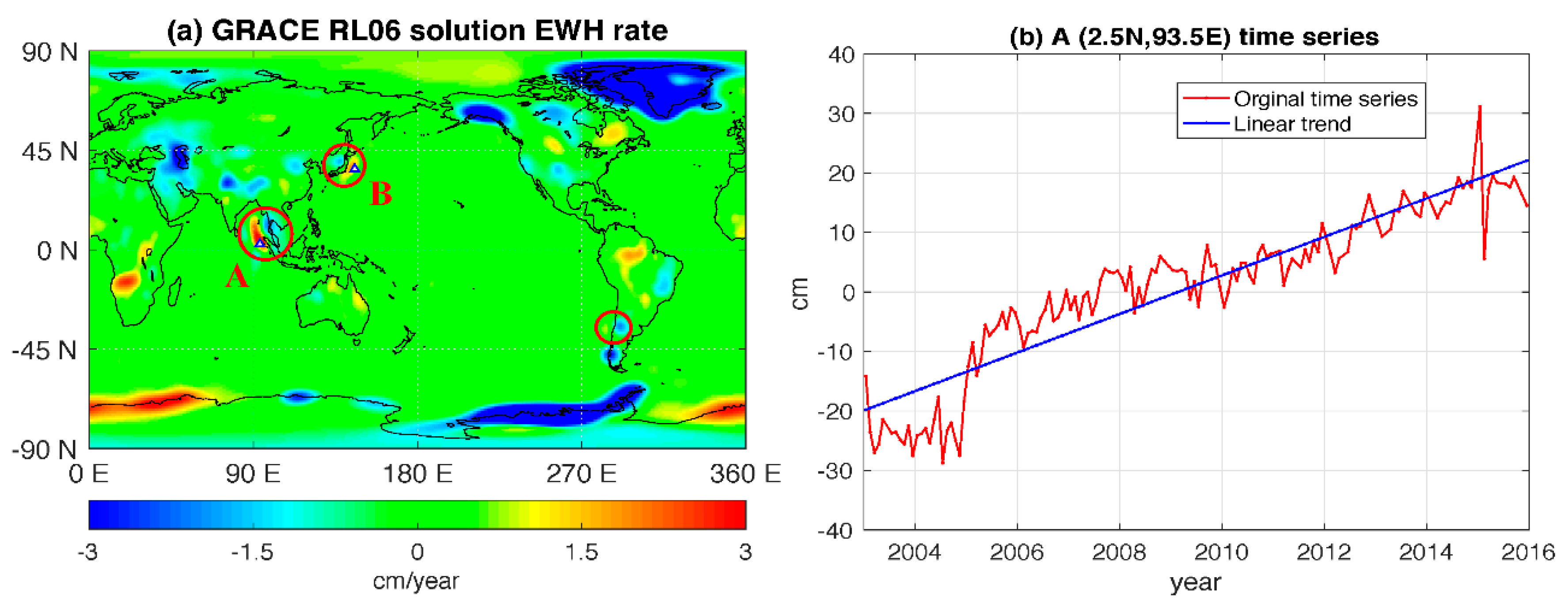
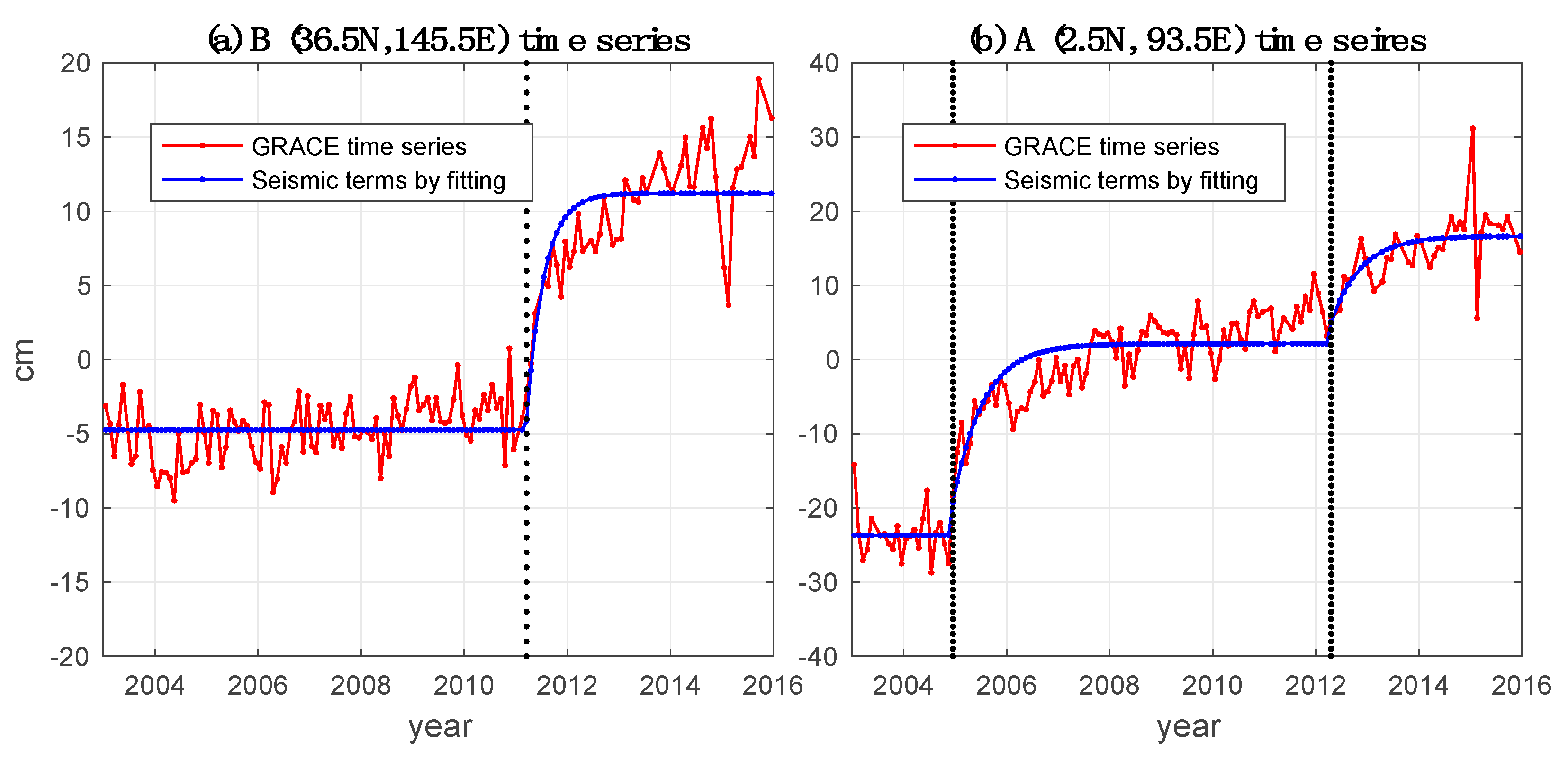
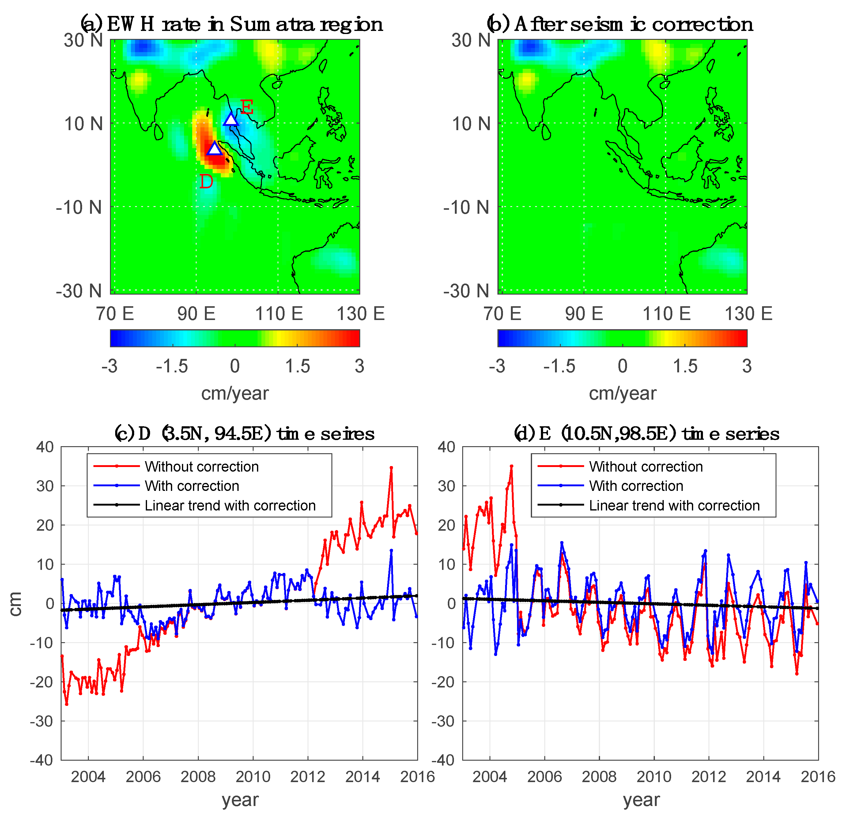
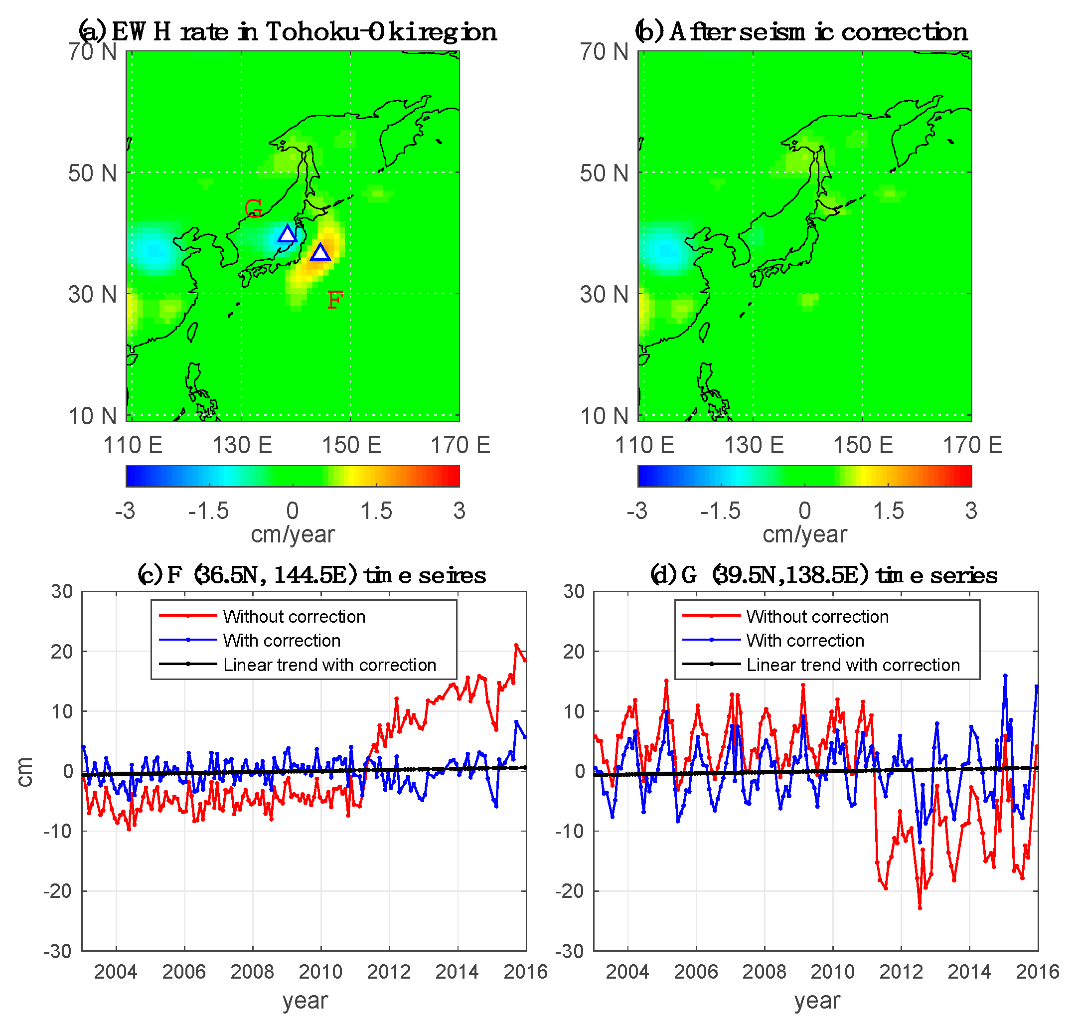
3. Results
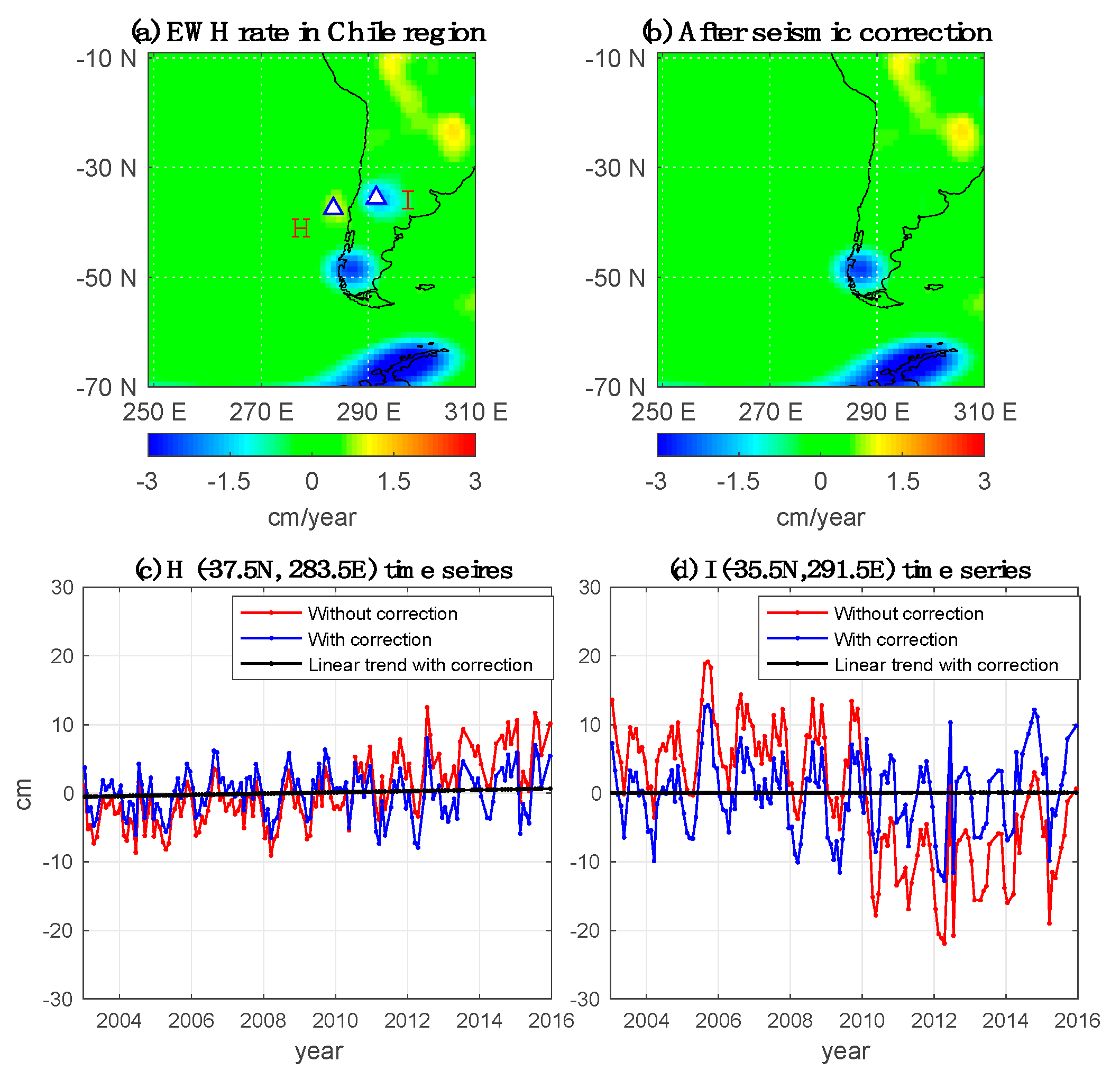
3.1. Seismic Effect Correction
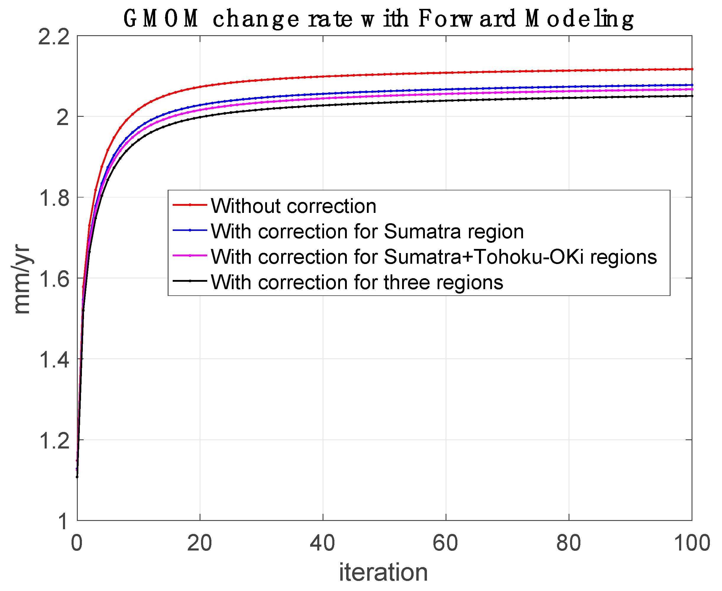
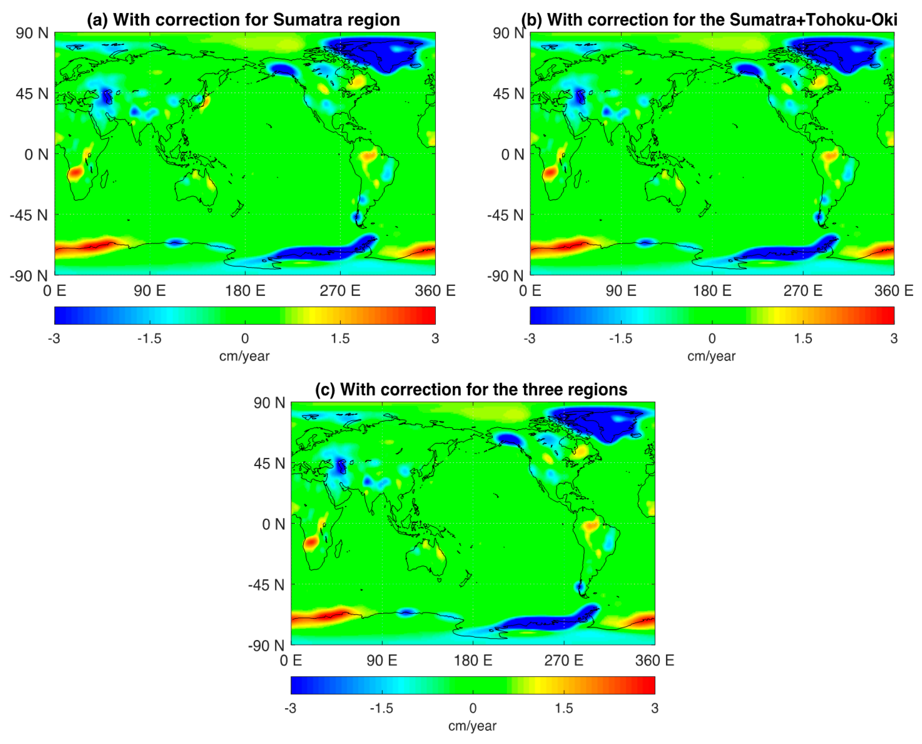
3.2. Impact of Seismic Effect on the GMOM Change Rate
4. Discussion
4.1. Uncertainty Estimate of GMOM Change Rate
4.2. Uncertainty Estimate of Seismic Impact on the GMOM Change Rate
4.3. Comparison with Estimates from Altimery and Argo
4.4. Seismic Impact for Shorter Time Spans and Regional Scales
5. Conclusions
Supplementary Materials
Author Contributions
Funding
Acknowledgments
Conflicts of Interest
References
- WCRP Global Sea Level Budget Group. Global sea-level budget 1993-present. Earth Syst. Sci. Data 2018, 10, 1551–1590. [Google Scholar] [CrossRef]
- The IMBIE Team. Mass balance of Greenland Ice Sheet from 1992 to 2018. Nature 2019. [Google Scholar] [CrossRef]
- The IMBIE Team. Mass balance of Antarctica Ice Sheet from 1992 to 2017. Nature 2019. [Google Scholar] [CrossRef]
- Wouters, B.; Gardner, A.S.; Moholdt, G. Global Glacier Mass Loss during the GRACE satellite Mission (2002–2016). Front. Earth Sci. 2019, 7, 96. [Google Scholar] [CrossRef]
- Reager, J.T.; Gardner, A.S.; Famiglietti, J.S.; Wiese, D.N.; Eicker, A.; Lo, M.-H. A decade of sea level rise slowed by climate-driven hydrology. Science 2016, 351, 699–703. [Google Scholar] [CrossRef]
- Dieng, H.B.; Cazenave, A.; von Schuckmann, K.; Ablain, M.; Meyssignac, B. Sea level budget over 2005–2013: Missing contributions and data errors. Ocean Science 2015, 11, 789–802. [Google Scholar] [CrossRef]
- Cazenave, A.; Palanisamy, H.; Ablain, M. Contemporary sea level changes from satellite altimetry: What have we learned? What are the new challenges? Adv. Space Res. 2018, 62, 1639–1653. [Google Scholar] [CrossRef]
- Chen, J.L.; Wilson, C.R.; Tapley, B.D. Contribution of ice sheet and mountain glacier melt to recent sea level rise. Nat. Geosci. 2013, 6, 549–552. [Google Scholar] [CrossRef]
- Chen, J.L.; Tapley, B.D.; Save, H.; Tamisiea, M.E.; Bettadpur, S.; Ries, J. Quantification of ocean mass change using gravity recovery and climate experiment, satellite altimeter, and Argo floats observations. J. Geophys. Res. Solid Earth 2018, 123, 10221–10225. [Google Scholar] [CrossRef]
- Dieng, H.B.; Cazenave, A.; Meyssignac, B.; Ablain, M. New estimate of the current rate of sea level rise from a sea level budget approach. Geophys. Res. Lett. 2017, 44, 3744–3751. [Google Scholar] [CrossRef]
- Xi, H.; Zhang, Z.; Lu, Y.; Li, Y. Mass sea level variation in the South China Sea from GRACE, altimetry and model and the connection with ENSO. Adv. Space Res. 2019, 64, 117–128. [Google Scholar] [CrossRef]
- Sun, Y.; Riva, R.; Ditmar, P. Optimizing estimates of annual variations and trends in geocenter motion and J2 from a combination of GRACE data and geophysical models. J. Geophys. Res. Solid Earth 2016, 121, 8352–8370. [Google Scholar] [CrossRef]
- Jeon, T.; Seo, K.W.; Youm, K.; Chen, J.L.; Wilson, C.R. Global sea level change signatures observed by GRACE satellite gravimetry. Sci. Rep. 2018, 8, 13519. [Google Scholar] [CrossRef] [PubMed]
- Chen, J.L.; Tapley, B.D.; Seo, K.-W.; Wilson, C.R.; Ries, J. Improved Quantification of Global Mean Ocean Mass Change Using GRACE Satellite Gravimetry Measurements. Geophys. Res. Lett. 2019, 46, 13984–13991. [Google Scholar] [CrossRef]
- Kim, J.-S.; Seo, K.-W.; Jeon, T.; Chen, J.L.; Wilson, C.R. Missing hydrological contribution to sea level rise. Geophys. Res. Lett. 2019, 46. [Google Scholar] [CrossRef]
- Wahr, J.; Zhong, S. Computations of the viscoelastic response of a 3-D compressible Earth to surface loading: An application to Glacial Isostatic Adjustment in Antarctica and Canada. Geophys. J. Int. 2013, 192, 557–572. [Google Scholar] [CrossRef]
- Peltier, R.W.; Argus, D.F.; Drummond, R. Comment on “An assessment of the ICE-6G_C (VM5a) glacial isostatic adjustment model” by Purcell et al. J. Geophys. Res. Solid Earth 2018, 123, 2019–2028. [Google Scholar] [CrossRef]
- Caron, L.; Ivins, E.R.; Larour, E.; Adhikari, S.; Nilsson, J.; Blewitt, G. GIA Model Statistics for GRACE Hydrology, Cryosphere, and Ocean Science. Geophys. Res. Lett. 2018, 45, 2203–2212. [Google Scholar] [CrossRef]
- Uebbing, B.; Kushce, J.; Rietbroek, R.; Landerer, F.W. Processing Choices Affect Ocean Mass Estimates from GRACE. J. Geophys. Res. Oceans 2019, 124, 1029–2044. [Google Scholar] [CrossRef]
- Han, S.C.; Riva, R.; Sauber, J.; Okal, E. Source parameter inversion for recent great earthquakes from a decade-long observation of global gravity fields. J. Geophys. Res. Solid Earth 2013, 118, 1240–1267. [Google Scholar] [CrossRef]
- Chao, B.F.; Liau, J.R. Gravity changes due to large earthquakes detected in GRACE satellite data via empirical orthogonal function analysis. J. Geophys. Res. Solid Earth 2019, 124, 3024–3035. [Google Scholar] [CrossRef]
- Han, S.C.; Shum, C.K.; Bevis, M.; Ji, C.; Kuo, C. Crustal dilatation observed by GRACE after the 2004 Sumatra-Andaman earthquake. Science 2006, 313, 658–661. [Google Scholar] [CrossRef]
- Han, S.C.; Sauber, J.; Riva, R. Contribution of satellite gravimetry to understanding seismic source processes of the 2011 Tohoku-Oki earthquake. Geophys. Res. Lett. 2011, 38, L24312. [Google Scholar] [CrossRef]
- Matsuo, K.; Heki, K. Coseismic gravity changes of the 2011 Tohoku-Oki earthquake from satellite gravimetry. Geophys. Res. Lett. 2011, 38, L00G12. [Google Scholar] [CrossRef]
- Han, S.C.; Sauber, J.; Luthcke, S. Regional gravity decrease after the 2010 Maule (Chile) earthquake indicates large-scale mass redistribution. Geophys. Res. Lett. 2010, 37, L23307. [Google Scholar] [CrossRef]
- Han, S.C.; Sauber, J.; Pollitz, F. Coseismic compression/dilatation and viscoelastic uplift/subsidence following the 2012 Indian Ocean earthquakes quantified from satellite gravity observations. Geophys. Res. Lett. 2015, 42. [Google Scholar] [CrossRef]
- Han, S.C.; Sauber, J.; Pollitz, F. Postseismic gravity change after the 2006–2007 great earthquake doublet and constraints on the asthenosphere structure in the central Kuril Islands. Geophys. Res. Lett. 2016, 43, 3169–3177. [Google Scholar] [CrossRef] [PubMed]
- Rahimi, A.; Li, J.; Naeeni, M.R.; Shahrisvand, M.; Fatolazadeh, F. On the extraction of co-seismic signal for the Kuril Island earthquakes using GRACE observations. Geophys. J. Int. 2018, 215, 346–362. [Google Scholar] [CrossRef]
- Tanaka, Y.-S.; Heki, K.; Matsuo, K.; Shestakov, N.V. Crustal subsidence observed by GRACE after the 2013 Okhotsk deep-focus earthquake. Geophys. Res. Lett. 2015, 42, 3204–3209. [Google Scholar] [CrossRef]
- Bettadpur, S. CSR Level-2 Processing Standards Document for Product Release 06, GRACE 327-742, Revision 5.0, The GRACE Project, Center for Space Research, University of Texas at Austin. Available online: https://podaac-tools.jpl.nasa.gov/drive/files/allData/grace/docs/L2-CSR006_ProcStd_v5.0.pdf (accessed on 18 April 2018).
- Wahr, J.; Molenaar, M.; Bryan, F. Time variability of the Earth’s gravity field: Hydrological and oceanic effects and their possible detection using GRACE. J. Geophys. Res. 1998, 103, 30205–30229. [Google Scholar] [CrossRef]
- Cheng, M.K.; Ries, J.R. Monthly Estimates of C20 from 5 SLR Satellites Based on GRACE RL06 Models, GRACE Technical Note 11, The GRACE Project, Center for Space Research, University of Texas at Austin. 2019. Available online: https://podaac-tools.jpl.nasa.gov/drive/files/allData/grace/docs/TN-11_C20_SLR.txt (accessed on 22 October 2019).
- Landerer, F. Monthly Estimates of Degree-1 (Geocenter) Gravity Coefficients, Generated from GRACE (04-2002–06/2017) and GRACE – FO (06/2018 onward) RL06 Solutions, GRACE Technical Note 13, The GRACE Project, NASA Jet Propulsion Laboratory. 2019. Available online: https://podaac-tools.jpl.nasa.gov/drive/files/allData/grace/docs/TN-13_GEOC_CSR_RL06.txt (accessed on 17 October 2019).
- Swenson, S.; Chambers, D.; Wahr, J. Estimating geocenter variations from a combination of GRACE and ocean model output. J. Geophys. Res. 2008, 113, B08410. [Google Scholar] [CrossRef]
- de Linage, C.; Rivera, L.; Hinderer, J.; Boy, J.-P.; Rogister, Y.; Lambotte, S.; Biancale, R. Separation of coseismic and postseismic gravity changes for the 2004 Sumatra–Andaman earthquake from 4.6 yr of GRACE observations and modelling of the coseismic change by normal-modes summation. Geophys. J. Int. 2009, 176, 695–714. [Google Scholar] [CrossRef]
- Li, J.; Chen, J.L.; Zhang, Z. Seismologic applications of GRACE time-variable gravity measurements. Earthq. Sci. 2014, 27, 229–245. [Google Scholar] [CrossRef]
- Chen, J.L.; Wilson, C.R.; Li, J.; Zhang, Z. Reducing leakage error in GRACE-observed long-term ice mass change: A case study in West Antarctica. J. Geod. 2015, 89, 925–940. [Google Scholar] [CrossRef]
- Dahle, C.; Flechtner, F.; Murböck, M.; Michalak, G.; Neumayer, H.; Abrykosov, O.; Reinhold, A.; König, R. GFZ Level-2 Processing Standards Document for Level-2 Product Release 06; GRACE 327-743, (Rev. 1.0), (Scientific Technical Report STR—Data; 18/04); GFZ German Research Centre for Geosciences: Potsdam, Germany, 2018. [Google Scholar] [CrossRef]
- Yuan, D.-N. JPL Level-2 Processing Standards Document for Product Release 06, GRACE 327-744, Revision 6.0, Jet Propulsion Laboratory, California Institute of Technology. Available online: https://podaac-ftp.jpl.nasa.gov/allData/grace/docs/L2-JPL_ProcStds_v6.0.pdf (accessed on 1 June 2018).
- Paulson, A.; Zhong, S.; Wahr, J. Inference of mantle viscosity from GRACE and relative sea level data. Geophys. J. Int. 2007, 171, 497–508. [Google Scholar] [CrossRef]
- Peltier, W.R.; Argus, D.F.; Drummond, R. Space geodesy constrains ice-age terminal deglaciation: The global ICE-6G_C (VM5a) model. J. Geophys. Res. Solid Earth 2015, 120, 450–487. [Google Scholar] [CrossRef]
- Li, J.; Chen, J.L.; Wilson, C.R. Topographic effects on coseismic gravity change for the 2011 Tohoku-Oki earthquake and comparison with GRACE. J. Geophys. Res. Solid Earth 2016, 121, 5509–5537. [Google Scholar] [CrossRef]


| Without Correction | With Correction for Sumatra Region | With Correction for Sumatra + Tohoku-Oki Regions | With Correction for the Three Regions | |
|---|---|---|---|---|
| GMOM rate (mm/yr) | 2.12 ± 0.11 * | 2.08 ± 0.12 * | 2.07 ± 0.12 * | 2.05 ± 0.12 * |
| Without Correction (mm/year) | With Correction (mm/year) | |
|---|---|---|
| CSR RL06 | 2.12 ± 0.11 | 2.05 ± 0.12 |
| GFZ RL06 | 2.05 ± 0.11 | 1.97 ± 0.11 |
| JPL RL06 | 2.16 ± 0.11 | 2.07 ± 0.11 |
© 2020 by the authors. Licensee MDPI, Basel, Switzerland. This article is an open access article distributed under the terms and conditions of the Creative Commons Attribution (CC BY) license (http://creativecommons.org/licenses/by/4.0/).
Share and Cite
Tang, L.; Li, J.; Chen, J.; Wang, S.-Y.; Wang, R.; Hu, X. Seismic Impact of Large Earthquakes on Estimating Global Mean Ocean Mass Change from GRACE. Remote Sens. 2020, 12, 935. https://doi.org/10.3390/rs12060935
Tang L, Li J, Chen J, Wang S-Y, Wang R, Hu X. Seismic Impact of Large Earthquakes on Estimating Global Mean Ocean Mass Change from GRACE. Remote Sensing. 2020; 12(6):935. https://doi.org/10.3390/rs12060935
Chicago/Turabian StyleTang, Lu, Jin Li, Jianli Chen, Song-Yun Wang, Rui Wang, and Xiaogong Hu. 2020. "Seismic Impact of Large Earthquakes on Estimating Global Mean Ocean Mass Change from GRACE" Remote Sensing 12, no. 6: 935. https://doi.org/10.3390/rs12060935
APA StyleTang, L., Li, J., Chen, J., Wang, S.-Y., Wang, R., & Hu, X. (2020). Seismic Impact of Large Earthquakes on Estimating Global Mean Ocean Mass Change from GRACE. Remote Sensing, 12(6), 935. https://doi.org/10.3390/rs12060935