Article

Optical Water Type Guided Approach to Estimate Optical Water Quality Parameters

1
Tartu Observatory, University of Tartu, 50090 Tartu, Estonia
2
Department of Marine Systems, School of Science, Tallinn University of Technology, 12616 Tallinn, Estonia
3
Estonian Marine Institute, University of Tartu, 12618 Tallinn, Estonia
*
Author to whom correspondence should be addressed.
Remote Sens. 2020, 12(6), 931; https://doi.org/10.3390/rs12060931
Submission received: 10 February 2020 / Revised: 9 March 2020 / Accepted: 11 March 2020 / Published: 13 March 2020

Abstract

:
Currently, water monitoring programs are mainly based on in situ measurements; however, this approach is time-consuming, expensive, and may not reflect the status of the whole water body. The availability of Multispectral Imager (MSI) and Ocean and Land Colour Instrument (OLCI) free data with high spectral, spatial, and temporal resolution has increased the potential of adding remote sensing techniques into monitoring programs, leading to improvement of the quality of monitoring water. This study introduced an optical water type guided approach for boreal regions inland and coastal waters to estimate optical water quality parameters, such as the concentration of chlorophyll-a (Chl-a) and total suspended matter (TSM), the absorption coefficient of coloured dissolved organic matter at a wavelength of 442 nm (aCDOM(442)), and the Secchi disk depth, from hyperspectral, OLCI, and MSI reflectance data. This study was based on data from 51 Estonian and Finnish lakes and from the Baltic Sea coastal area, which altogether were used in 415 in situ measurement stations and covered a wide range of optical water quality parameters (Chl-a: 0.5–215.2 mg·m−3; TSM: 0.6–46.0 mg·L−1; aCDOM(442): 0.4–43.7 m−1; and Secchi disk depth: 0.2–12.2 m). For retrieving optical water quality parameters from reflectance spectra, we tested 132 empirical algorithms. The study results describe the best algorithm for each optical water type for each spectral range and for each optical water quality parameter. The correlation was high, from 0.87 up to 0.93, between the in situ measured optical water quality parameters and the parameters predicted by the optical water type guided approach.

Graphical Abstract

1. Introduction

Remote sensing offers effective ways to observe spatial and/or temporal variations in water quality, which is vital for the comprehensive assessment and management of water bodies [1]. Currently, water monitoring programs are mainly based on in situ measurements; however, considering that water bodies are dynamic in nature, this method may not reflect the status of the whole water body. Therefore, it is important to implement techniques that allow more effective monitoring of the aquatic environment. However, remote sensing of inland and coastal waters can be challenging as they are independently influenced by different optically significant constituents (OSC)-coloured dissolved organic matter (CDOM), phytoplankton, and total suspended matter (TSM). All of these OSCs shape the spectral characteristics that are measured by the remote sensor.
Phytoplankton consists of single-celled, free-floating, photosynthetic organisms that form the base of the aquatic food web, being an important component of the carbon cycle. Seasonal phytoplankton blooms are natural processes in the aquatic environment [2]. However, a rise in phytoplankton biomass may also be a sign of eutrophication, which indicates increased nutrient inputs [3,4], all of which, in turn, leads to drastic changes in the aquatic ecosystem (e.g., altered species composition, hypoxia, decreased water transparency, toxins, problems for fishes) [5,6]. The photosynthetic phytoplankton pigment chlorophyll-a (Chl-a) is typically used as a proxy for phytoplankton biomass [7]. Chl-a absorbs strongly in the blue (440–500 nm) and red (650–680 nm) regions of the visible spectrum and reflects in the green (550 nm) [8]. Remote sensing algorithms for the retrieval of Chl-a are based on the ratios of reflectance, such as the blue-green ratio [9], which are empirically related to the Chl-a concentration. However, this is not valid for optically complex waters, where CDOM and TSM also affect the optical properties of water. Several studies have suggested the use of various combinations of near-infrared (NIR) and red band combinations instead [10,11,12].
TSM is used as an indicator of physical forcing, for instance, wind-driven resuspension, land runoff, as well as dredging operations, which lead to much higher TSM concentrations in the area [13,14]. TSM is divided into suspended particulate organic matter (SPOM) and suspended particulate inorganic matter (SPIM). SPOM contains a mixture of planktonic organisms (e.g., phytoplankton, bacterioplankton, etc.,) and non-living organic matter, and the optical properties are similar to those of CDOM [15]. The presence of terrigenous particles in the water often accounts for the bulk of SPIM. SPIM scatters light, whereas the scattering depends on the size and shape of the particles—particles < 1 µm scatter more strongly at shorter wavelengths, while in the case of larger particles, the wavelength dependence is weak [15,16]. This limits the accuracy of algorithms for estimating TSM. The use of red and/or NIR wavelengths is suggested to quantify the SPIM part due to strong water absorption in the NIR wavelengths [17].
CDOM is an optically active fraction of dissolved organic matter [18]. It may have a local origin, for instance, from degradation of phytoplankton cells, or it may be advected from a distant source, for example, from organic-rich rivers. CDOM can be used as a proxy for assessing dissolved organic carbon dynamics, identifying organic pollution in agricultural and urban catchments, and detecting influences of anthropogenic activities (e.g., land-use change) [19]. Light absorption by CDOM tends to be the strongest at shorter wavelengths (350–450 nm) of the electromagnetic spectrum. Absorbance increases exponentially with decreasing wavelengths and diminishes to near-zero in the red wavelength region [20]. Therefore, the water-leaving reflectance at 440 nm is often used to estimate CDOM from remote sensing data [21,22].
Secchi disk depth (ZSD) is a measure of water transparency or of the depth of penetration of visible light in the aquatic environment, which is relevant for primary production [23]. The lower the Secchi disk depth value, the more turbid and less clear the water. Substances that influence the transparency of water include phytoplankton, CDOM, and suspended matter (i.e., OSCs). Therefore, changes in the ZSD also reflect variations in the water properties. Many regional algorithms have been developed to estimate ZSD from remote sensing reflectance. For optically complex waters, different spectral band combinations between blue, green, and red bands are often used [24,25].
The launches of Multispectral Imager (MSI) and Ocean and Land Colour Instrument (OLCI) on board Sentinel-2 and Sentinel-3, respectively, have increased the potential for improved monitoring of water quality. MSI was primarily designed to support land monitoring for Europe’s environmental monitoring Copernicus programme, but owing to its high spatial resolution (10, 20, and 60 m), with 13 spectral bands [26], it has opened new opportunities to investigate smaller water bodies [27] and different phenomena in more detail (e.g., filaments and eddies of biological activity) [28,29]. OLCI, on the other hand, is specially designed for water quality monitoring. It is a follow-up of the MERIS (Medium Resolution Imaging Spectrometer) mission, with improved capabilities. It has a 300 m spatial resolution with 21 spectral bands optimised to measure ocean colour over optically complex water bodies [26].
Different approaches have been used to evaluate water quality products from these sensors [30,31,32,33]. In the case of optically complex waters, where optical properties are more diverse and can vary over short spans of time and space, standard remote sensing products often fail [30,34,35,36], which has led to the development of regionally specific algorithms [37]. However, regional algorithms also do not show consistency in terms of changes in their optical properties [30]. The possible solution could be to use remote sensing algorithms based on the classification of the optical water types (OWTs). For instance, a similar OWT-based solution was also used to interpret data from the first satellite ocean color sensor Coastal Zone Color Scanner (CZCS) [38,39], where the classification of OWTs by Morel and Prieur [40] was used for the separation of water masses. Using remote sensing to classify waters according to their optical properties will help to identify relationships between different OSCs and to understand the biogeochemical processes therein. Several studies have developed optical pre-classification schemes to select regional algorithms for water quality parameters [41,42,43,44]. Uudeberg et al. [45] developed an OWT classification based on reflectance spectral features for boreal inland and coastal waters. This classification divides waters into five OWTs dominated by Chl-a, TSM, or CDOM, and the classification is compatible with data from OLCI and MSI. This OWT classification forms the base of this study.
The main aim was to find a solution for boreal region inland and coastal waters to estimate optical water quality parameters from reflectance spectra as an alternative to standard algorithms that do not work in this region. For this, we chose the OWT guided approach and tested various published empirical algorithms to find the best algorithm for every OWT for different spectral ranges for different optical water quality parameters. Our study included optical water quality parameters, such as the concentration of Chl-a and TSM, the absorption coefficient of CDOM at a wavelength of 442 nm (aCDOM(442)), the Secchi disk depth; and spectral ranges, such as in situ measured hyperspectral reflectance with 1 nm steps, the OLCI, onboard the Sentinel-3 satellite, bands, and the MSI, onboard the Sentinel-2 satellite, bands. Since there are still many problems associated with the removal of the atmospheric influence from satellite imagery; this work is based on in situ measured reflectance spectra and in situ measured reflectance spectra convolved into OLCI and MSI bands using sensor spectral response functions. Furthermore, the OWT guided approach was later applied to OLCI images to map the OWT guided approach and selected algorithms’ strengths and weaknesses.

2. Materials and Methods

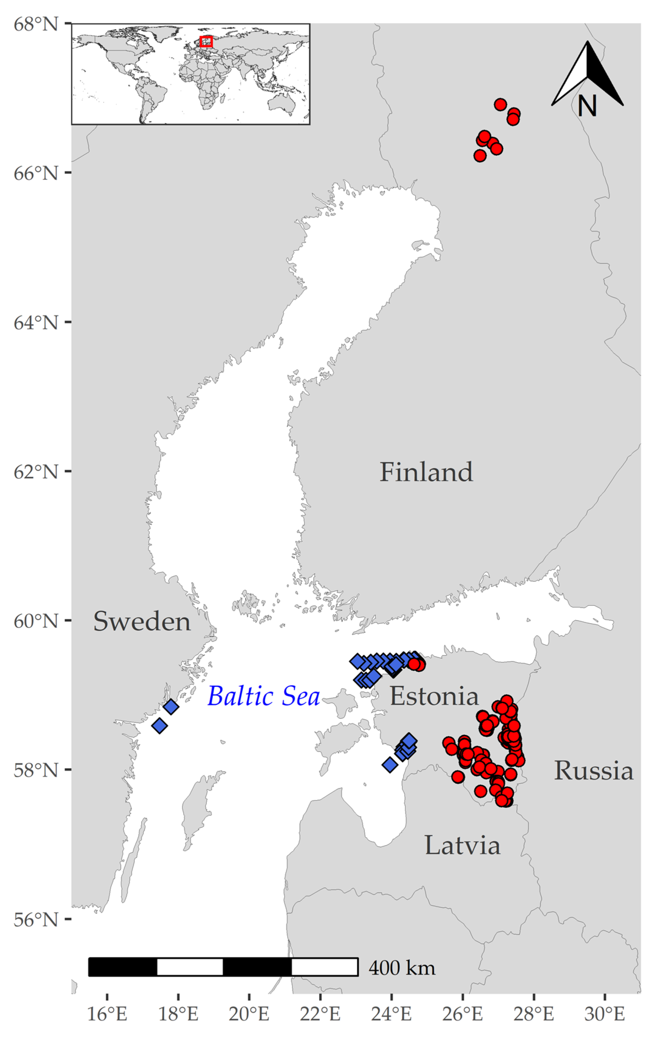
2.1. Study Sites and In Situ Dataset

This study was based on data from 415 in situ measurement stations gathered from the boreal region inland and coastal waters from April to September in 2012–2019. Data were collected from 51 different Estonian and Finnish lakes and from three coastal locations in the Baltic Sea (Figure 1). The first area in the Baltic Sea was Pärnu Bay, located on the west coast of Estonia, where the mean depth is 4.7 m (maximum 8 m) and the water is well mixed. Since Pärnu Bay is shallow, open to winds, and has sandy, clayey, and muddy bottom, wind-derived resuspension can lead to quite high and changeable TSM concentrations. The second area is located in the Gulf of Finland region, where the mean depth is 37 m, with a maximum of 123 m (Paldiski Deep), and where the water column is vertically stratified [16]. The area is prone to upwelling and downwelling events in the summer and autumn [46,47]. The third area is located in the Western Gotland Basin close to the coast of Sweden. The Baltic Sea reaches its greatest depth in the Western Gotland Basin, Landsort Deep (459 m), but in our measurement stations, the water depth was up to 30 m. In situ lake data were mainly collected from Estonian lakes (42 lakes), from small lakes, such as Lake Holstre (0.04 km2), to large lakes, such as Lake Peipsi (3555 km2); from lakes with highly transparent water, such as Lake Nohipalo Valgjärv (Secchi disk depth 5 m), to lakes with very brown-water, such as Nohipalo Mustjärv (Secchi disk depth 0.3 m) (Figure 2).
The in situ dataset contains data from measurements of water-leaving reflectance (R(λ)), concentrations of OSC (such as the concentration of Chl-a and TSM, and aCDOM(442)), Secchi disk depth, and different environment parameters, such as wind speed, waves heights, cloudiness, and sun condition. The Secchi disk depths were measured on the shadowed side of the vessel with a white disk with a 30 cm diameter or with a 20 cm diameter white disk with holes. The wind speed was measured with a handheld mechanical anemometer. The wave height, cloudiness, and sun condition were estimated by visual inspection.

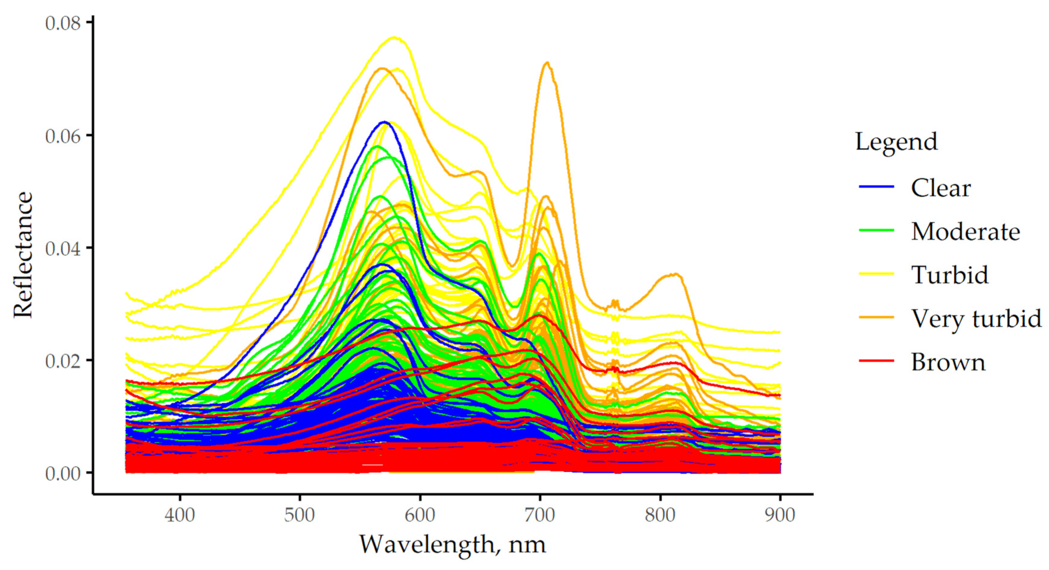
2.1.1. Water-Leaving Reflectance (R(λ))

R(λ) was measured with TriOS-RAMSES hyperspectral radiometers using two different setups. The first setup was used in 233 in situ measurement stations and the second setup was used on 182 in situ measurement stations.
For the first setup, the above the water system consisted of three TriOS-RAMSES hyperspectral radiometers: two radiance sensors measuring upwelling radiance (Lt(λ)) and downwelling radiance (Lsky(λ)) in the same azimuthal plane, and one irradiance sensor measuring downwelling irradiance (Ed(λ)) [48]. The radiance sensor’s nadir/zenith angles of 40° were fixed in the frame. The measured spectral range was 350–900 nm. The recording interval was once per 10-second interval. The solar azimuth angle was kept between 90° and 180° and was adjusted manually during measurements. The calculation of R(λ) followed the protocol of REVAMP [48] and included the next steps. First, all measured radiance and irradiance spectra were linearly interpolated to a 1 nm step. Secondly, R(λ) was calculated as
R ( λ ) = π L t ( λ ) ρ ( w ) L s k y ( λ ) E d ( λ ) ,
where ρ ( w ) is the sea surface reflectance as function of wind speed (w, m·s−1) and calculated as ρ ( w ) = 0.0256 + 0.00039 w + 0.000034 w 2 [48]. Finally, the median R(λ) was calculated and used as the representative of the measurement station.
For the second setup, the profiling system consisted of two TriOS-RAMSES hyperspectral radiometers: one irradiance sensor measuring downwelling irradiance (Ed(λ)) and one radiance sensor measuring upwelling radiance (Lu(λ)). Measurements were made above the water, below the water surface, and at different depths in the water column. In this study, only above-the-water measurements were used. The measured spectral range was 350–900 nm. At every depth, five recordings were made. The R(λ) calculations included three steps. First, all measured spectra were linearly interpolated to a 1 nm step. Secondly, R(λ) was calculated as
R ( λ ) = π L u ( λ ) E d ( λ ) .
Finally, the median R(λ) was calculated and used as the representative of the in situ measurement station.
To study the implementation capacity of the OWT guided approach for retrieving water quality parameters, the R(λ) spectra representing the in situ measurement stations were also convolved into MSI and OLCI bands using spectral response functions (SRFs) of satellite sensor bands and calculated according to Uudeberg et al. [45]. The SRFs for the MSI and OLCI were taken from [49] and [50], respectively.

2.1.2. Analysis of Water Samples

Water samples for measurements of the concentrations of OSC were collected from the water surface (up to 0.5 m depth) according to ISO 5667-3 [51] and analysed according to ISO 10260 [52]. After the samples were filtered through Whatman GF/F filters that retain fine particles down to 0.7 μm, and the pigments were extracted with 5 ml of 96% ethanol, the concentrations of Chl-a were measured spectrophotometrically with a Hitachi U-3010 spectrophotometer and calculated according to Jeffrey and Humphrey [53]. After the samples were filtered through a filter with a pore size of 0.2 µm, CDOM was measured in a 5 cm optical cuvette against distilled water with a Hitachi U-3010 spectrophotometer and calculated according to Lindell et al. [54]. The concentrations of TSM were measured gravimetrically after the samples were filtered through pre-washed, pre-ashed, and pre-weighed Whatman GF/F filters.
The water samples collected during July 2018 in the Gulf of Finland had some differences in analysis. For TSM, a fixed amount of water (0.750 L) was filtered through pre-combusted and pre-weighted Millipore membrane filters with a pore size of 0.45 µm. For Chl-a, the Thermo Helios γ spectrophotometer was used and the concentrations of Chl-a were calculated according to Lorenzen [55].

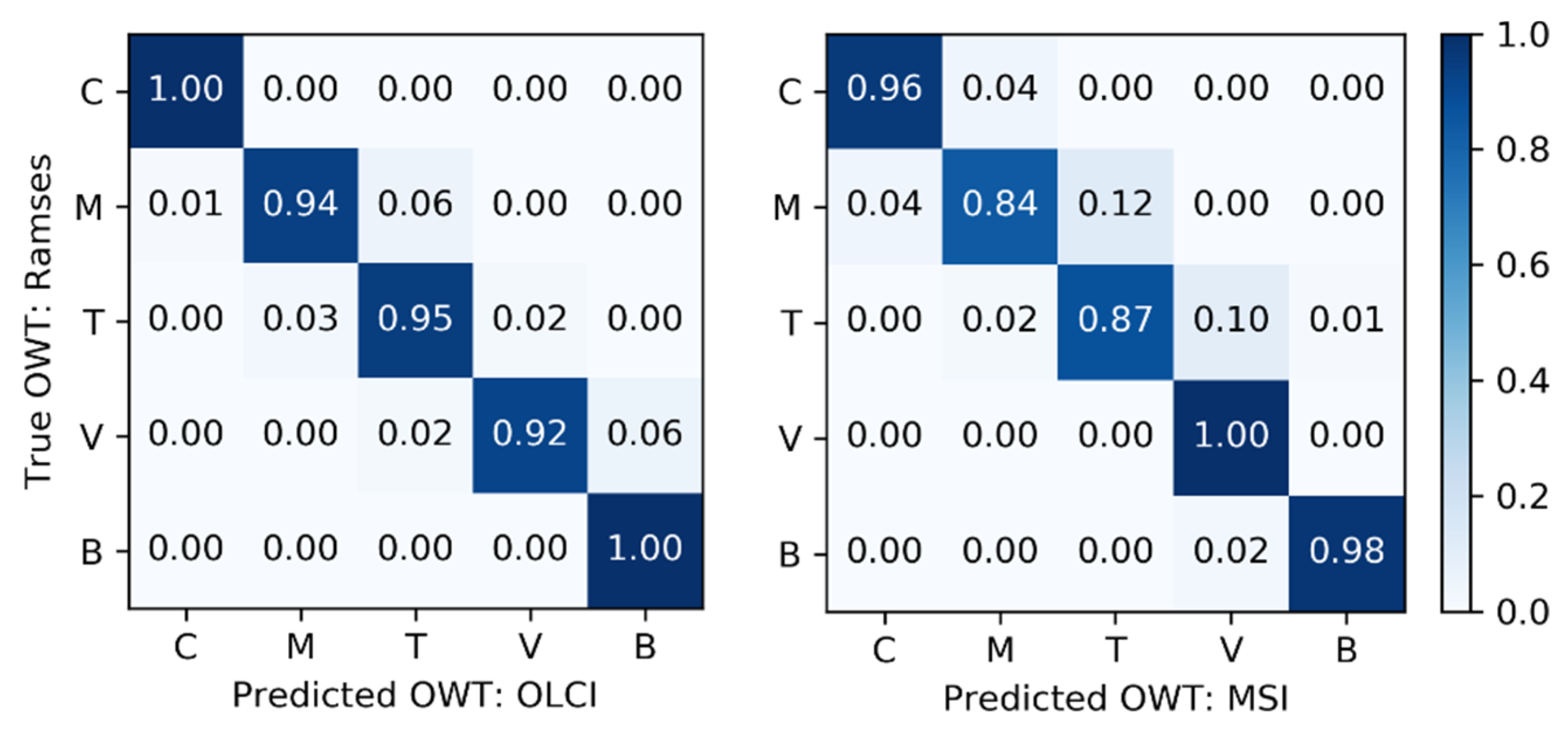
2.2. Classification of Optical Water Types (OWTs)

The classification of OWTs introduced by Uudeberg et al. [45] was used to determine the OWT. The classification divides the boreal region inland and coastal waters into five OWTs, each linked to the specific bio-optical condition in order to reflect the dominance of group OSC concentrations. The Clear OWT corresponds to water with the highest transparency and lowest OSC concentrations. In the Moderate OWT, the concentrations of OSC have risen, but none of them dominate. In the Turbid OWT, the TSM is the dominant OSC and the R(λ) values are the highest. In the Very Turbid OWT, Chl-a is the dominant OSC. The strong Chl-a peak, which is associated with blooms, occur in the red part of spectra. The Brown OWT water is dominated by CDOM.
The OWT classification is based on reflectance spectra key features, such as the wavelength of the maximum, the slopes, and the amplitude of R(λ). The maximum likelihood of individual spectra to reference spectra using a combination of spectral correlation similarity and modified spectral angle similarity was used to determine the OWT for measured R(λ) spectra. The OWTs were assigned on each in situ measurement of R(λ) and the in situ measurements of R(λ) convolved into MSI and OLCI sensor bands.

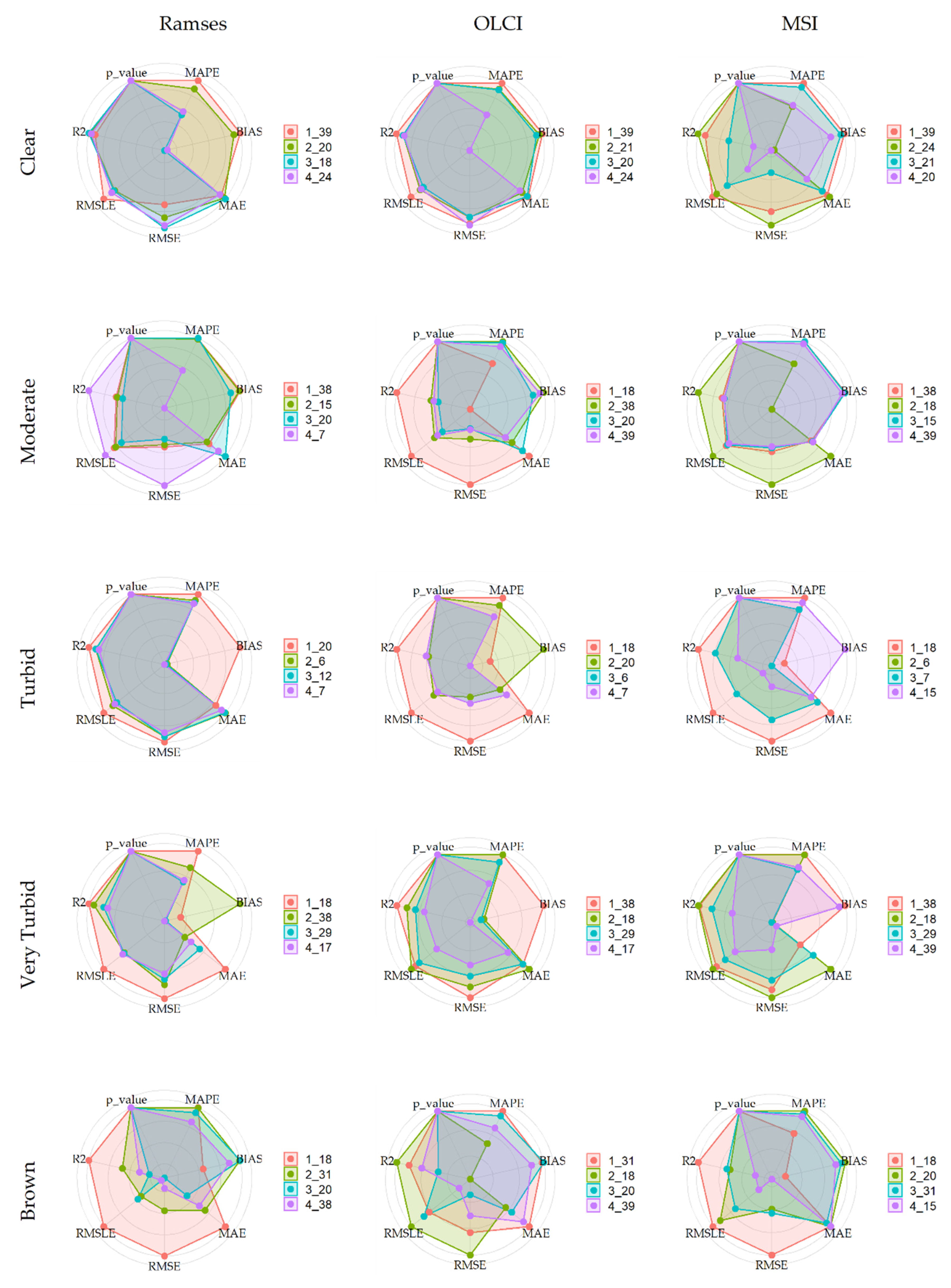
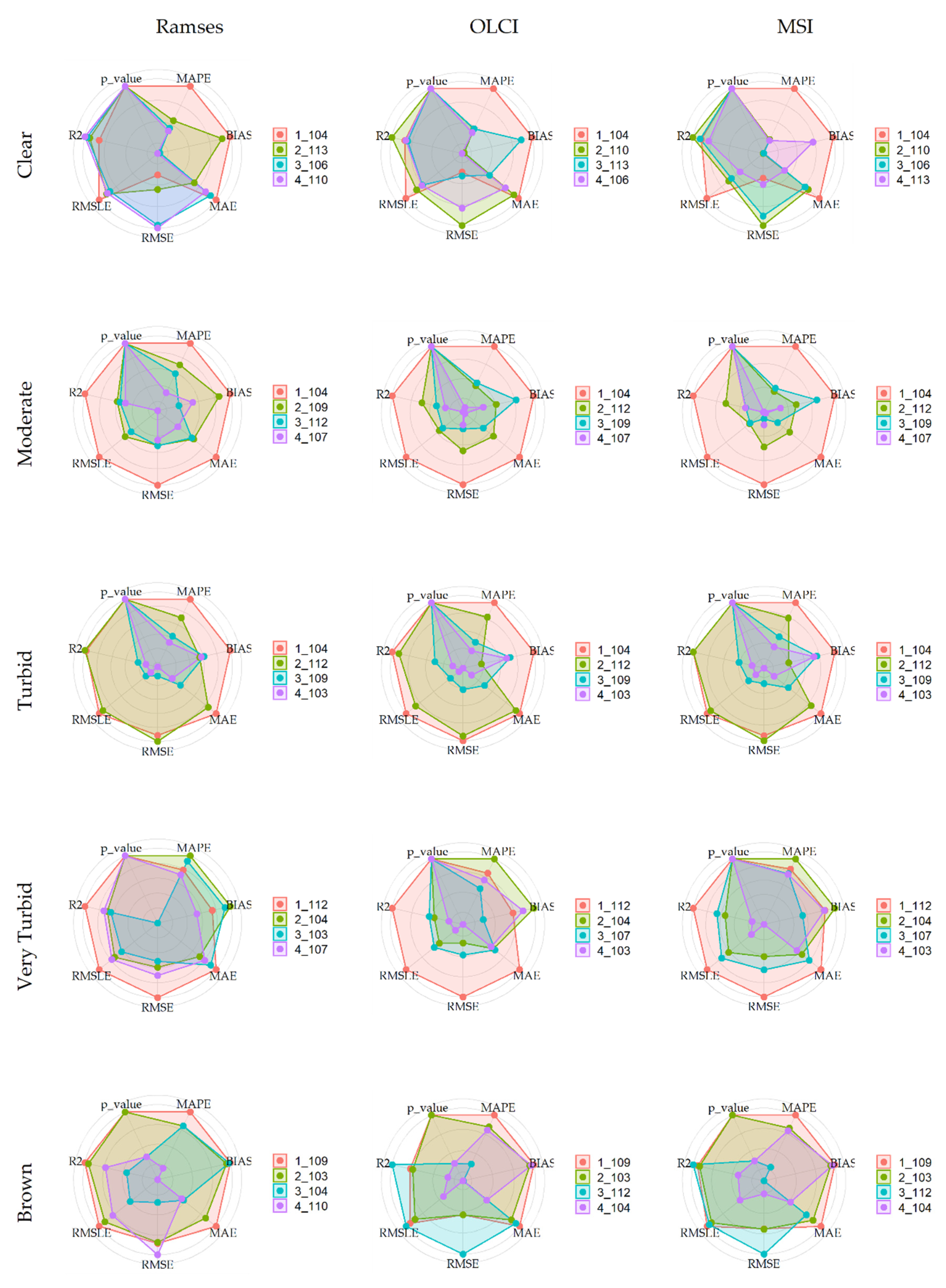
2.3. Algorithms for Retrieving Water Quality Parameters

OWT guided approach was used for finding models for retrieving water quality parameters, such as the concentration of Chl-a, the concentration of TSM, the aCDOM(442), and Secchi disk depth, from R(λ) spectra. Since the inland and coastal waters are optically complex and cover large variations of OSC concentrations, the OWT guided approach allows to find the best model for different bio-optical conditions. In this study, we used 132 previously published algorithms from manuscripts that were available for us, including 60 for Chl-a, 39 for TSM, 21 for CDOM, and 12 for Secchi disk depth. Details of used algorithms are shown in Appendix A Table A1.
Repeated K-fold Cross-validation [56] was the statistical method to build and select the model using published algorithms for optical water quality parameter and the R package caret [57] by Max Kuhn was used for implementation. The Repeated K-fold Cross-validation contains following steps: (1) the data are divided randomly into k folds of equal size; (2) the k-1 folds are used for the model training; (3) the hold-out fold is used for the model validation; and (4) steps (1)–(3) are repeated n times. Finally, based on a selected statistical metric, the model with the best average score is assigned as the final model. Ten folds, ten repeats, and the root mean squared error as metrics were used in this study.
The ranking system used a combination of scaled and threshold-based statistical metrics to select the model for retrieving the optical water quality parameter from R(λ) per OWTs. Statistical metrics, such as RMSE, RMSLE, MAE, MAPE, and BIAS, were scaled from 0 (maximum value) to 1 (minimum value); the R2 was scaled from 0 (minimum value) to 1 (maximum value); and for the p-value, the thresholds were used as 1 for p-value under 0.001, 0.5 for p-value between 0.001 and 0.05, and 0, when p-value was over 0.05. Finally, all values were summed up and the model with the highest score was selected as the model for future retrievals. The following statistical metrics were used in this study and they are described in detail in R package Metrics [58].
  • RMSE (Root Mean Squared Error)—represents the average difference between the measured values and the values predicted by the model. This metric indicates the fit of the model to the data. The lower the RMSE, the better the model.
  • RMSLE (Root Mean Squared Logarithmic Error)—represents the average difference between the log-transformed measured values and the log-transformed values predicted by the model. This metric does not penalize big differences when both the predicted and the measured values are big numbers. This is useful when the measurement values are in a wide range. The lower the RMSLE, the better the model.
  • MAE (Mean Absolute Error)—represents the average absolute difference between the measured and predicted model values. This metric measures the model prediction error and is robust against the effect of outliers. The lower the MAE, the better the model.
  • MAPE (Mean Absolute Percentage Error)—measures the average absolute percentage error from the measured value and the values predicted by the model divided by the measured value. This metrics shows the model prediction accuracy. The lower the MAPE, the better the model.
  • R2—represents the squared correlation between the measured values and the predicted values by the model. This metric shows the percentage of variance explained by the model. The closer to 1 the R2, the better the model.
  • BIAS—represents the average amount by which the measured value is greater than predicted. The lower the bias, the better the model.
  • p-value—tests the null hypothesis and shows if the model is statistically significant or not. A low p-value (<0.05) suggests that the model is statistically significant.
To find the best solutions also for the MSI and OLCI sensors R(λ) spectral range, all calculations were made separately on R(λ) spectra range with a 1 nm step, R(λ) spectra convolved into OLCI sensor bands, and R(λ) spectra convolved into MSI sensor bands. Since the OLCI and MSI band locations were sometimes different than the band locations described in algorithms, the closest possible band was selected in case of OLCI or MSI were lacking exact bands.

2.4. Satellite Dataset
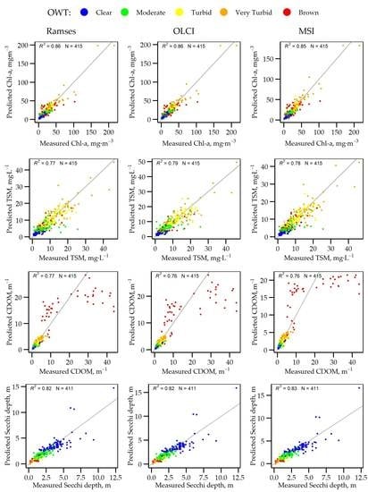
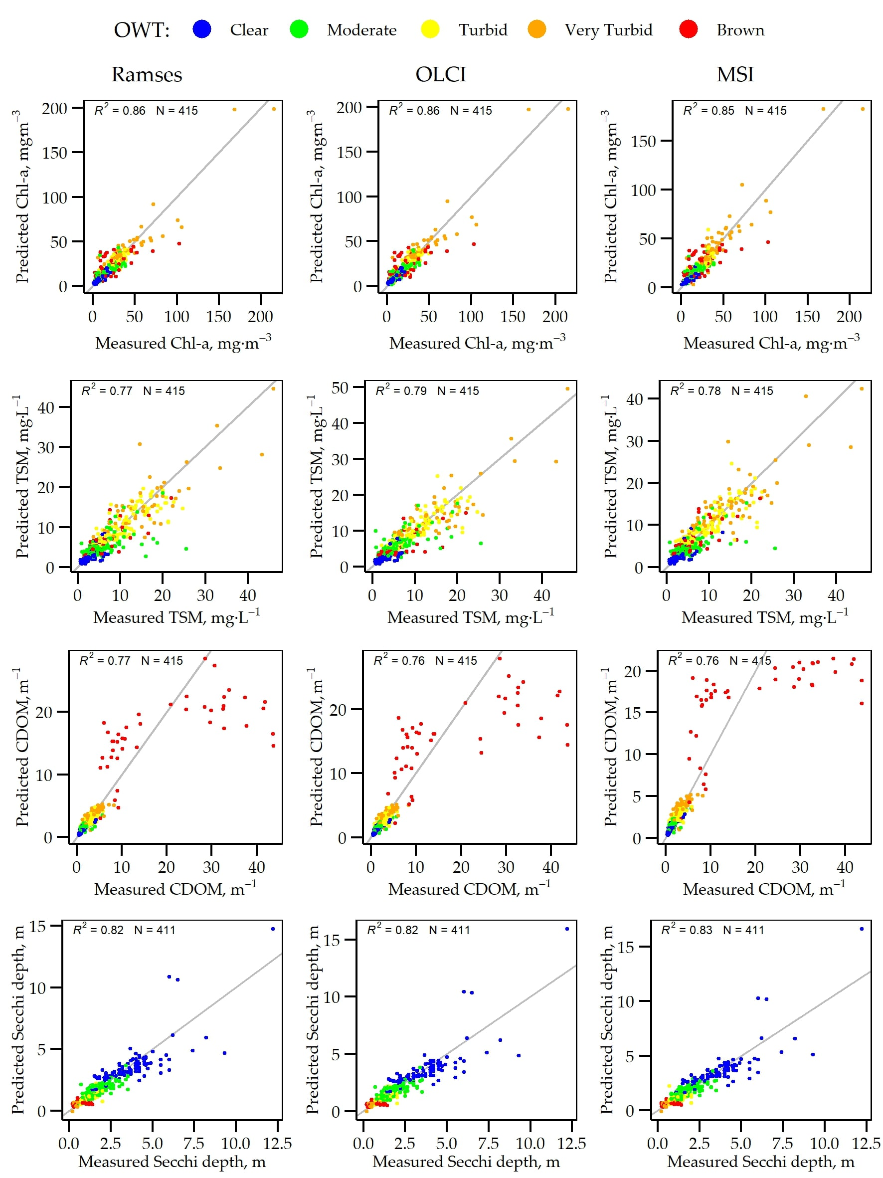
To assess the ability of the OWT guided approach to obtain optical water quality parameters from satellite data, the full resolution Level-1 images acquired in 2018 and 2019 by OLCI, onboard the Sentinel-3 satellite, were used. Level-1 images were processed with the Case-2 Regional CoastColour (C2RCC) atmospheric correction processor v1.15, based on the previous study’s recommendation [45]. Image primary processing, such as subsetting the region of interest and atmospheric correction processing, and downloading was done using the ESTHub Processing Platform, which is the Estonian Land Board’s national mirror site for Copernicus satellite data and processing [59]. After that, the OWT were determined for every pixel of the satellite images. Finally, the OWT-based models described in Table 2, Table 3, Table 4 and Table 5 were used to find the optical water quality parameters.

3. Results

3.1. Description of In Situ Dataset

Our in situ dataset from 415 in situ measurement stations covers wide ranges of the OSC concentrations and Secchi disk depth. However, datasets of all four parameters are significantly non-Gaussian. Table 1 shows the skewness of Chl-a and CDOM are 4.3 and 4.1, respectively. This indicates that their distributions are not symmetrical and are skewed strongly towards higher values. Moreover, Table 1 allows us to assume based on the high maximum and median values of the Chl-a, CDOM, and Secchi disk depth, that the dataset includes also measurements from extreme optical conditions for the boreal region. For example, the high transparency (Secchi disk depth up to 12.2 m) was measured in July in the Gulf of Finland during an upwelling event. Therefore, water masses with different properties (low OSC concentrations, high transparencies, and cold temperatures (~4 °C)) were present compared to the usual situations. High CDOM values around 40 m−1 were measured multiple times through the vegetation period in dark-water small Estonian lakes. Chl-a values of 215.2 mg·m−3 and 168.4 mg·m−3 were captured during the blooming situation in large Lake Peipsi. However, in the dataset, there is a lack of measurement stations where the TSM was dominated by mineral particles. For instance, the median proportion of suspended particulate organic matter in TSM is 76%.
Figure 3 shows the in situ measured R(λ) at 415 stations classified into various OWTs, and Figure 4 shows the range of the variations of the OSC concentrations and Secchi disk depth for OWTs. The OWT for each in situ measured R(λ) was determined by the maximum likelihood of the individual spectrum to type averages. The Clear OWT was assigned to the R(λ) of 100 measurement stations. The maxima of R(λ) were between 540 and 580 nm and the mean maximum value was 0.012. Waters were the most transparent (maximum Secchi disk depth 12.2 m) and with the lowest OSC concentrations. However, in Figure 3, one Clear OWT station has a too high maximum value at 550 nm (0.06) compared to the rest of the Clear OWT spectra, but inspection of the station OSC concentration does not confirm a misclassification. The Moderate OWT was the most frequent in our dataset, with the R(λ) of 124 stations being assigned to this OWT. The Turbid OWT was assigned to the R(λ) of 98 measurement stations. This OWT is dominated by TSM and the highest TSM values were expected to be in this OWT. However, in this dataset, the highest TSM values were in stations assigned to the Very Turbid OWT. TSM is mainly dominated by SPOM in our dataset, and especially in these high TSM valued Very Turbid OWT stations (88% of TSM was SPOM). These waters are generally dominated by Chl-a, and stations are classified correctly. The Very Turbid OWT was assigned to the R(λ) of 51 measurement stations, which were dominated by Chl-a. The Brown OWT was assigned to the R(λ) of 42 stations. These stations had very low R(λ) values (median value 0.003), with maxima in the red part of the spectrum, and very high aCDOM(442) values with a median at 13.6 m−1.
The accuracies of OWT estimations, based on in situ measurements of R(λ) convolved into MSI and OLCI sensor bands using sensor-specific SRFs, were 96% for OLCI and 91% for MSI. As the goal was to use the OWT guided approach to retrieve optical water quality parameters, it was important to understand the capability to assign the same OWT on in situ measurements of R(λ) regardless of spectral scale (Ramses with 1 nm step resolution, and distinct bands for OLCI and MSI). Confusion matrices were constructed between the OWTs assigned on in situ measurements of R(λ) (set as the true OWT value) and those which were assigned based on in situ measurements of R(λ) convolved into various sensor bands (set as the predicted OWT value). As shown in Figure 5, the OLCI confusion matrix demonstrates a strong distinction for Clear and Brown OWTs (100% correct assignment) and the highest rate of misclassification in Very Turbid OWT, with 8% of spectra being misclassified as Brown or Turbid OWT. The MSI confusion matrix illustrates a strong distinction for Very Turbid, and Brown OWTs (100% and 98% correct assignment respectively); however, 16% of Moderate OWT spectra were misclassified.

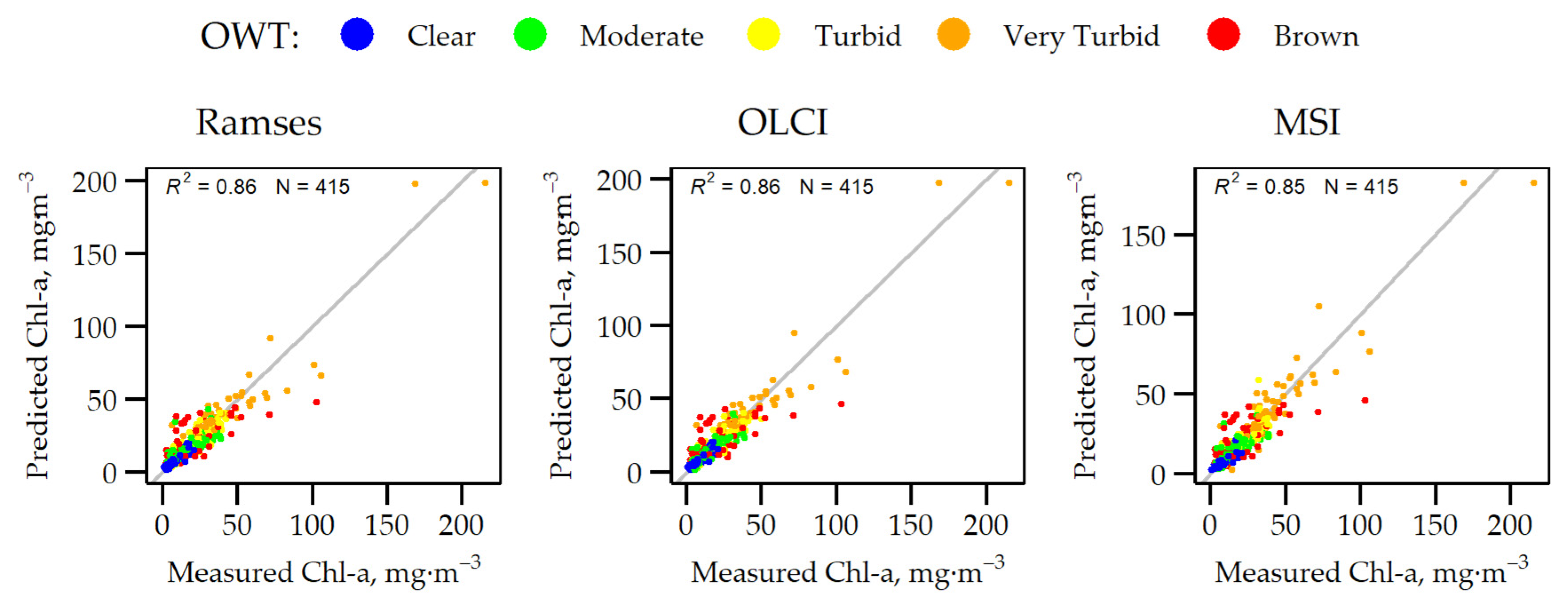
3.2. Predictive Models for Concentration of Chlorophyll-a (Chl-a)

The best models to retrieve the concentration of Chl-a from the R(λ) spectra for each OWT and each spectral ranges, such as Ramses with 1 nm step, and OLCI and MSI bands, are defined in Table 2. We tested 60 published empirical algorithms to retrieve the Chl-a values and the best ones for all the cases were chosen based on our model ranking system described in paragraph 2.3. As a result, the four best models for each OWT and each spectral range are shown on radar plots in Appendix B Figure A1. The linear regression models showed a better performance for all the cases.
For the Clear OWT, in the case of Ramses and OLCI, the model CHL69 using the Gitelson et al. [60] algorithm had the highest score, and, for MSI, the model using the MERIS maximum chlorophyll index by Gower et al. [61] was the most suitable. The model CHL97 using the Mishra and Mishra [62] algorithm was the best for Moderate OWT for Ramses and in Very Turbid OWT, for all the different spectral ranges. For Turbid OWT, all three spectral ranges were described best with different models with different approaches: for Ramses, the model using the Kutser et al. [63] algorithm based on two-band ratio approach; for OLCI, the model using the Gitelson et al. [64] algorithm based on a three-band approach, and for MSI, the model using the Zimba and Gitelson [11] four-band approach. For Brown OWT, retrieving the concentration of Chl-a from R(λ) was the most difficult and the coefficient of determination suggested that the regression model explained about 40% of the variance observed in the in situ measured data. However, all models were statistically significant based on the p-values.
The correlations shown in Figure 6, between the concentration of Chl-a predicted using OWT based models and in situ measured concentration of Chl-a, were strong, such as 0.93 for Ramses and OLCI, and 0.92 for MSI. Overall, the predicted concentrations of Chl-a were the most accurate compared to other optical water quality parameters explored in this study.
Table 2. The best published chlorophyll-a (Chl-a) predictive models tested in this study for each optical water types (OWT) and for sensors with different spectral scales. Descriptions of the algorithms used for these models are found in Table A1, and the acronyms and abbreviations are in Table A2. The band central wavelength is used to mark the Ocean and Land Colour Instrument (OLCI) and Multispectral Imager (MSI) models bands.
OWTModelModel FormulaST 1R2p-value
Ramses
ClearCHL69 C h l a = 5956.0 · ( R 709 R 665 + R 754 2 ) + 3.84 LR0.79< 2.2E-16
ModerateCHL97 C h l a = 84.42 · ( ( 1 R 705 1 R 665 ) / ( 1 R 705 + 1 R 665 ) ) + 18.69 LR0.62< 2.2E-16
TurbidCHL88 C h l a = 55.85 · ( R 702 R 674 ) 43.08 LR0.79< 2.2E-16
Very TurbidCHL97 C h l a = 180.6 · ( ( 1 R 705 1 R 665 ) / ( 1 R 705 + 1 R 665 ) ) + 19.89 LR0.88< 2.2E-16
BrownCHL67 C h l a = 46.56 · ( R 748 R 667 ) 8.310 LR0.414.3E-06
OLCI
ClearCHL69 C h l a = 6097.2 · ( R 708.75 R 665 + R 753.75 2 ) + 3.998 LR0.78< 2.2E-16
ModerateCHL65 C h l a = 33.91 · ( R 673.75 R 708.75 ) + 54.07 LR0.67< 2.2E-16
TurbidCHL98 C h l a = 177.4 · ( 1 R 673.75 1 R 708.75 ) · R 753.75 + 20.68 LR0.79< 2.2E-16
Very TurbidCHL97 C h l a = 173.6 · ( ( 1 R 708.75 1 R 665 ) / ( 1 R 708.75 + 1 R 665 ) ) + 25.6 LR0.89< 2.2E-16
BrownCHL67 C h l a = 42.96 · ( R 753.75 R 665 ) 5.470 LR0.385.9E-06
MSI
ClearCHL101 C h l a = 4367.1 · ( R 705 R 665 705 665 740 665 · ( R 740 R 665 ) ) + 2.658 LR0.61< 2.2E-16
ModerateCHL65 C h l a = 40.83 · ( R 665 R 705 ) + 61.71 LR0.60< 2.2E-16
TurbidCHL57 C h l a = 184.1 · ( R 740 R 705 R 740 R 665 ) + 21.20 LR0.63< 2.2E-16
Very TurbidCHL65 C h l a = 171.4 · ( R 665 R 705 ) + 183.6 LR0.89< 2.2E-16
BrownCHL67 C h l a = 46.98 · ( R 740 R 665 ) 9.360 LR0.406.0E-06
1 Statistical technique.

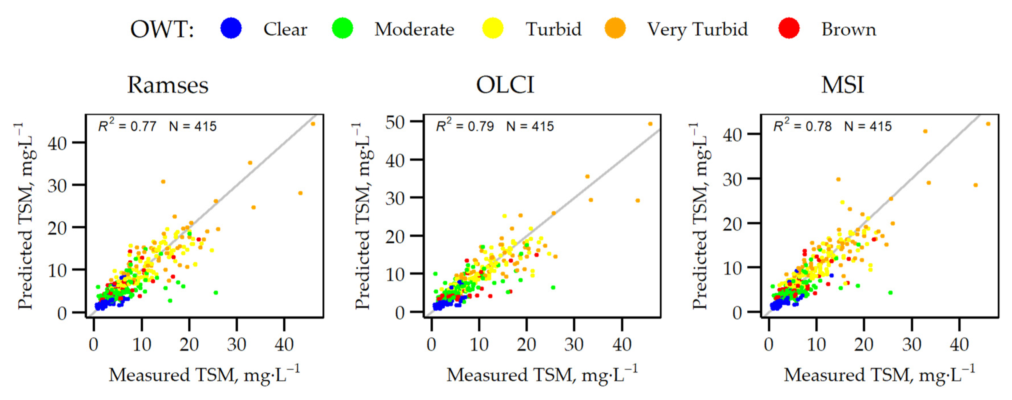
3.3. Predictive Models for Concentration of Total Suspended Matter (TSM)

The best models to retrieve the concentrations of TSM from R(λ) spectra for each OWT and for each spectral range are defined in Table 3. We tested 39 published empirical algorithms to retrieve the concentrations of TSM. The model TSM18 using the Kutser et al. [65] algorithm based on the reflectance spectra peak at 810 nm was the most well represented based on our models ranking system results. This model suited well for the MSI sensor, where it had the highest score for Turbid, Very Turbid, and Brown OWTs and according to Figure A2, for the Moderate OWT, it had the second place due to its low bias contribution. Model TSM18 had high scores for Ramses and the OLCI spectral scale for Turbid, Very Turbid, and Brown OWTs. For the Clear OWT, the model TSM39 using Zhang et al. [66] developed log-transformed multiple linear regression algorithm, based on a combination of 488, 555, and 645 nm information, was the best for all sensors. The Moderate OWT had the lowest coefficient of determination for all the spectral ranges from all the OWTs; however, all models were statistically significant based on p-values.
The correlations between concentrations of TSM predicted using OWT based models and in situ measured concentrations of TSM values were strong: 0.87, 0.89, 0.88 for Ramses, OLCI, and MSI respectively. However, Figure 7 shows that model tends to underestimate strongly points with high TSM values (from 15 to 25 mg·L−1), present in Moderate OWT.
Table 3. The best published total suspended matter (TSM) predictive models tested in this study for each optical water type (OWT) and for sensors with different spectral scales. Descriptions of the algorithms used for these models are found in Table A1, and acronyms and abbreviations, in Table A2. The band central wavelength is used to mark the Ocean and Land Colour Instrument (OLCI) and Multispectral Imager (MSI) models bands.
OWTModelModel FormulaST 1R2p-value
Ramses
ClearTSM39 log T S M = 30.20 · R 555 + 74.14 · R 645 0.991 · R 488 R 555 + 0.784 LT-MLR0.475.7E-13
ModerateTSM38 log T S M = 0.264 · log R 555 + 14.71 · R 645 0.189 · log R 488 R 555 + 0.941 LT-MLR0.361.5E-11
TurbidTSM20 ln T S M = 0.685 · ln R 620 · R 681 R 510 + 4.852 LLR0.69< 2.2E-16
Very TurbidTSM18 T S M = 3748.6 · ( R 810 R 770 + R 840 2 ) + 5.515 LR0.689.8E-14
BrownTSM18 T S M = 5673.9 · ( R 810 R 770 + R 840 2 ) + 2.178 LR0.618.4E-10
OLCI
ClearTSM39 log T S M = 24.36 · R 560 + 80.66 · R 665 1.096 · R 490 R 560 + 0.840 LT-MLR0.473.5E-13
ModerateTSM18 T S M = 8090.1 · ( R 865 R 778.75 + R 865 2 ) + 1.825 LR0.45< 2.2E-16
TurbidTSM18 T S M = 7664.9 · ( R 865 R 778.75 + R 865 2 ) + 3.250 LR0.69< 2.2E-16
Very TurbidTSM38 log T S M = 0.249 · log R 560 + 26.20 · R 665 0.483 · log R 490 R 560 + 0.095 LLR0.604.0E-09
BrownTSM31 ln T S M = 311.8 · ( R 708.75 R 753.75 + R 665 2 ) + 1.165 LT-LR0.492.0E-07
MSI
ClearTSM39 log T S M = 24.0 · R 560 + 79.02 · R 665 1.152 · R 490 R 560 + 0.892 LT-MLR0.494.0E-14
ModerateTSM38 log T S M = 0.279 · log R 560 + 16.24 · R 665 0.215 · log R 490 R 560 + 0.958 LT-MLR0.363.4E-10
TurbidTSM18 T S M = 7037.6 · ( R 783 R 783 + R 865 2 ) + 3.464 LR0.64< 2.2E-16
Very TurbidTSM18 T S M = 5416.1 · ( R 783 R 783 + R 865 2 ) + 6.259 LR0.68< 2.2E-16
BrownTSM18 T S M = 7573.5 · ( R 783 R 783 + R 865 2 ) + 2.748 LR0.541.8E-08
1 Statistical technique.

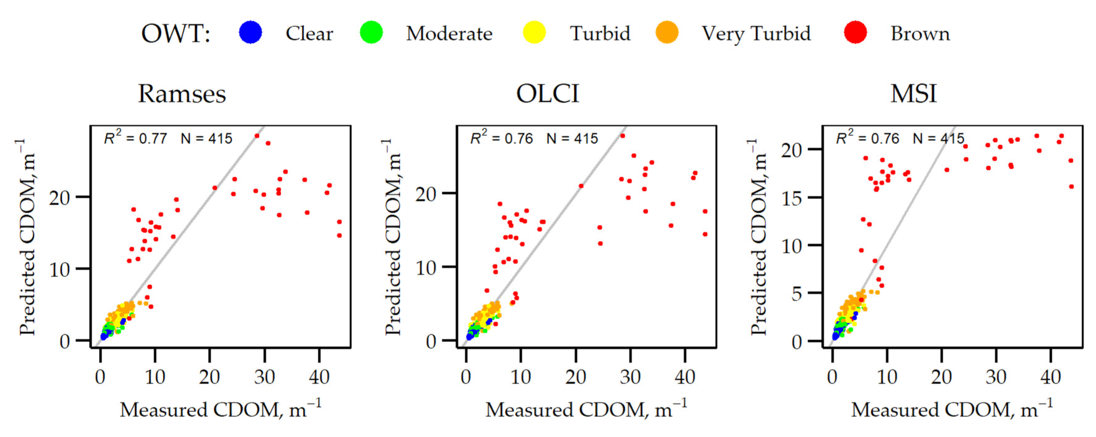
3.4. Predictive Models for Absorption Coefficient of Coloured Dissolved Organic Matter (CDOM)

The best models to retrieve the aCDOM(442) from the R(λ) spectra for each OWT and for each spectral range, are defined in Table 4. We tested 21 published empirical algorithms to retrieve the CDOM values. The power regression models (referred also as a log–log regression model) of the reflectance ratio showed better performance for all the spectral ranges in Clear, Moderate, and Turbid OWTs. For instance, the reflectance ratio 665/560 nm described by Menken et al. [67] was the best for OLCI and MSI; however, for Ramses, the model using the ratio 560/660 nm had the highest score. For the Very turbid OWT, the linear regression model CDOM119, using the Ammenberg et al. [68] algorithm, was the best for all spectral ranges. Furthermore, this model received high scores also in Clear, Moderate, and Turbid OWTs for OLCI and MSI, as shown in Figure A3. For the Brown OWT, the log-transformed multiple linear regression models had the best performance; however, this time the model for MSI used different reflectances compared to other spectral ranges. The p-value showed that all models were statistically significant, but only the Clear OWT coefficient of determination suggested that the regression model explained 74% of the variance observed in the in situ measured data.
The correlations between the predicted aCDOM(442), using OWT based models, and the in situ measured aCDOM(442) were strong, 0.88 for Ramses and 0.87 for both OLCI and MSI. Still, as shown in Figure 8, the capability to estimate the Brown OWT high CDOM values over 20 m−1 was non-existent and needs future investigation.
Table 4. The best published coloured dissolved organic matter (CDOM) predictive models tested in this study for each optical water type (OWT) and for sensors with different spectral scales. Descriptions of the algorithms used for these models are found in Table A1, and the acronyms and abbreviations, in Table A2. The band central wavelength is used to mark the Ocean and Land Colour Instrument (OLCI) and Multispectral Imager (MSI) models bands.
OWTModelModel FormulaST 1R2p-value
Ramses
ClearCDOM131 ln C D O M = 1.4124 · ln ( R 560 R 660 ) + 1.042 LLR0.74< 2.2E-16
ModerateCDOM124 ln C D O M = 1.470 · ln ( R 570 R 655 ) + 1.111 LLR0.361.4E-13
TurbidCDOM124 ln C D O M = 2.187 · ln ( R 570 R 655 ) + 1.225 LLR0.454.2E-14
Very TurbidCDOM119 C D O M = 3.063 · R 664 R 550 + 1.096 LR0.422.3E-07
BrownCDOM117 ln C D O M = 107.8 · R 485 0.245 · R 485 830 + 3.371 LT-MLR0.388.1E-05
OLCI
ClearCDOM122 ln C D O M = 1.352 · ln ( R 665 R 560 ) + 1.070 LLR0.74< 2.2E-16
ModerateCDOM122 ln C D O M = 1.108 · ln ( R 665 R 560 ) + 1.070 LLR0.337.1E-12
TurbidCDOM122 ln C D O M = 1.490 · ln ( R 665 R 560 ) + 1.265 LLR0.326.8E-10
Very TurbidCDOM119 C D O M = 3.128 · R 665 R 560 + 1.266 LR0.382.3E-06
BrownCDOM117 ln C D O M = 127.6 · R 485 0.140 · R 485 830 + 3.377 LT-MLR0.411.6E-05
MSI
ClearCDOM122 ln C D O M = 1.429 · ln R 665 R 560 + 1.059 LLR0.74< 2.2E-16
ModerateCDOM122 ln C D O M = 1.330 · ln R 665 R 560 + 1.086 LLR0.421.6E-14
TurbidCDOM122 ln C D O M = 1.338 · ln R 665 R 560 + 1.151 LLR0.311.9E-09
Very TurbidCDOM119 C D O M = 3.292 · R 665 R 560 + 0.947 LR0.398.7E-08
BrownCDOM133 ln C D O M = 62.93 · R 665 0.020 · R 560 R 490 + 3.107 LT-MLR0.412.2E-05
1 Statistical technique.

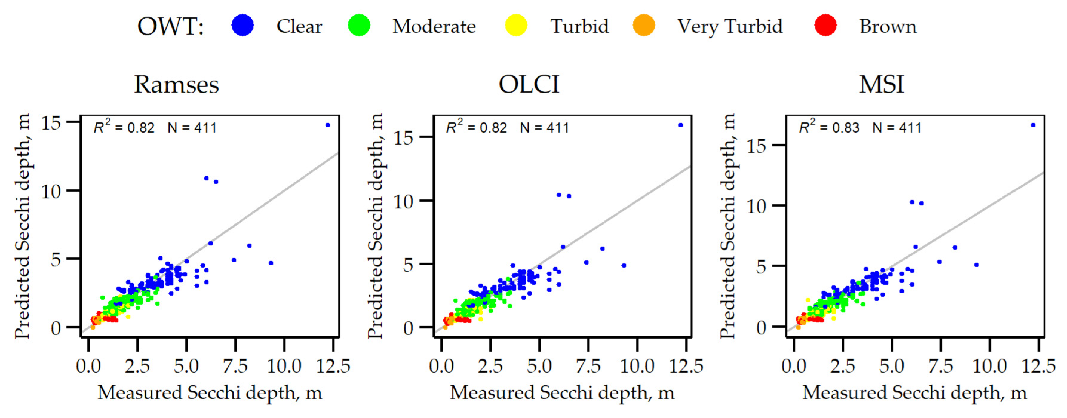
3.5. Predictive Models for Secchi Disk Depth

The best models to retrieve the Secchi disk depth value from R(λ) spectra for each OWT and for each sensor with different spectral ranges are defined in Table 5. We tested 12 published empirical algorithms to retrieve the Secchi disk depth. The model ZSD104, using the Kloiber et al. [69] algorithm based on log-transformed multiple regression of form 485/660 nm ratio and the additional 485 nm, had the best performance based on our ranking system. In all spectral ranges, the ZSD104 model was the best for Clear, Moderate, and Turbid OWTs and was also in the top four models for Very Turbid and Brown OWTs, as shown in Figure A4. For Very Turbid OWT, the model ZSD112 using Wu et al. [70] algorithm, based on multiple linear regression of five variables, had the highest score for all spectral ranges. For the Brown OWT, retrieving the Secchi disk depth from R(λ) was the most difficult and the highest correlation of all tested models was with ZSD109 using Hellweger et al. [71] algorithm, based on the reflectance at 660 nm. However, the coefficient of determination was around 0.28, but a p-value lower than 0.0005 shows that the model is still statistically significant.
Correlations between the Secchi disk depth predicted using OWT based models and the in situ measured Secchi disk depth values were strong, 0.91 for all the tested spectral ranges. However, as shown in Figure 9, some higher Clear OWT Secchi disk depth estimations from the R(λ) spectra had a lower accuracy. These in situ measurements were made during an upwelling event in the Gulf of Finland.
Table 5. The best Secchi disk depth predictive models using published algorithms tested in this study for each optical water types (OWT) and for sensors with different spectral scales. Descriptions of the algorithms used for building models are found in Table A1, and the acronyms and abbreviations, in Table A2. The band central wavelength is used to mark the Ocean and Land Colour Instrument (OLCI) and Multispectral Imager (MSI) models bands.
OWTModelModel FormulaST 1R2p-value
Ramses
ClearZSD104 ln S D D = 0.617 · R 485 R 660 43.58 · R 485 + 0.759 LT-MLR0.60< 2.2E-16
ModerateZSD104 ln S D D = 1.685 · R 485 R 660 63.01 · R 485 0.265 LT-MLR0.64< 2.2E-16
TurbidZSD104 ln S D D = 2.98 · R 485 R 660 41.32 · R 485 1.294 LT-MLR0.74< 2.2E-16
Very TurbidZSD112 S D D = 5.63 e 07 · ln R 555 R 488 0.018 · R 645 + R 858 R 469 15.57 · R 555 + 1.07 MLR0.489.6E-07
BrownZSD109 ln S D D = 0.268 · ln R 660 + 1.024 LLR0.270.0005
OLCI
ClearZSD104 ln S D D = 0.573 · R 490 R 665 42.89 · R 490 + 0.742 LT-MLR0.62< 2.2E-16
ModerateZSD104 ln S D D = 1.801 · R 490 R 665 60.42 · R 490 0.510 LT-MLR0.65< 2.2E-16
TurbidZSD104 ln S D D = 2.960 · R 490 R 665 39.95 · R 490 1.451 LT-MLR0.69< 2.2E-16
Very TurbidZSD112 S D D = 7.03 e 06 · ln R 560 R 490 0.027 · R 645 + R 858 R 469 14.63 · R 555 + 1.08 MLR0.481.6E-06
BrownZSD109 ln S D D = 0.269 · ln R 665 + 1.037 LLR0.280.0003
MSI
ClearZSD104 ln S D D = 0.602 · R 490 R 665 45.09 · R 490 + 0.728 LT-MLR0.64< 2.2E-16
ModerateZSD104 ln S D D = 1.821 · R 490 R 665 63.25 · R 490 0.478 LT-MLR0.68< 2.2E-16
TurbidZSD104 ln S D D = 2.784 · R 490 R 665 38.22 · R 490 1.367 LT-MLR0.63< 2.2E-16
Very TurbidZSD112 S D D = 6.81 e 06 · ln R 560 R 490 0.030 · R 645 + R 858 R 469 17.11 · R 555 + 1.14 MLR0.519.7E-09
BrownZSD109 ln S D D = 0.271 · ln R 665 + 1.033 LLR0.290.0002
1 Statistical technique.

4. Discussion

Our OWT guided approach to estimate optical water quality parameters, such as Chl-a, TSM, CDOM, and Secchi disk depth, from R(λ) spectra, can be the solution to monitor boreal region inland and coastal waters health operatively. Water bodies can vary in shape, size, depth, and also by water colour. As shown in Table 1, our in situ dataset from 52 different water bodies demonstrates that the optical water quality parameters can vary largely. For example, the concentration of the Chl-a range was from 0.5 to 215.2 mg·m−3, the TSM range was from 0.6 to 46.0 mg·L−1, the range for aCDOM(442) was 0.4 to 43.7 m−1, and for the Secchi disk depth the range was from 0.2 to 12.2 m. Therefore, to assume to find one algorithm per optical water quality parameter to fit with a good accuracy for all the water bodies may be a bit too optimistic.
Optically complex waters are independently influenced by Chl-a, TSM, and CDOM [8]. Therefore, these can be the reasons why standard remote sensing algorithms often fail in optically complex waters [72,73], and there are many regional or waterbody based [25,65,70,74,75] empirical algorithms. However, optical properties can vary strongly even inside one waterbody, for instance, during the one day in Lake Peipsi the concentration of Chl-a varied from 16.8 to 215.2 mg·m−3, and in addition there is seasonal and interannual variability; therefore, studies have suggested, that more detailed approach would be beneficial [76,77]. The use of OWT guided approach, which first classifies water into different OWTs, reflecting different bio-optical conditions, and then applies that OWT specific algorithm to estimate the optical water quality parameters, may be one of the possible solutions.
In the context of selecting the best empirical algorithm for predicting the optical water quality parameter from R(λ) spectra, this study showed, as expected, that the choice depends on the OWT and also the sensor spectral range. As the R(λ) spectra are the basis for all the future calculations and developments, the error in R(λ) may multiply in the final product or lead to incorrect conclusions [78]. Moreover, it is known that atmospheric correction over inland and coastal areas is difficult [79,80,81] and the result still can contain large errors [30,45,77,82,83]. Therefore, in this study, to eliminate as many errors as possible and focus on finding the best algorithm, we used in situ measured R(λ) spectra with 1 nm step and for OLCI and MSI we recalculated in situ measured R(λ) using SRFs into OLCI and MSI bands. The same approach has been used before [65]. However, it is still important to remember that in situ measured R(λ) is not the absolute truth and can contain large errors for example due to variable weather conditions [45,84,85,86]. For example, R(λ) measurements are difficult to perform well in CDOM-rich waters, which often leads to strong overestimation in the blue region of the spectrum [45,65]. Moreover, the presence of sunlight increases the R(λ) values in the blue part of the spectrum.
Linear regression models were used for predicting the concentration of Chl-a. Compared to other optical water quality parameter model selections, Chl-a varies the most between OWTs and the spectral range. The widely used [10,63,68,87,88,89,90,91,92] ratio 700/670 nm with a high correlation for high-biomass waters, was the best model only for Turbid OWT with a Ramses spectral range. However, the two variables ratio approach was the best for all the spectral ranges in Brown OWT, OLCI and MSI Moderate OWT, Ramses Turbid OWT, and MSI Very Turbid OWT. Matthews [93] suggests for lower Chl-a concentrations to use the ratio of the blue and green. In our best-performing models, all variables were selected from the red and NIR spectral range, with different combinations. Moreover, broadly used [10,30,61,87,94,95] algorithms that include chlorophyll fluorescence information using values of reflectance spectra around 681 nm were not the best for any cases. The Brown OWT retrieving models coefficients of determination were about 40%, thus needing future investigation and improvement.
From the 39 tested empirical algorithms to retrieve the concentration of TSM, the model TSM18 using the Kutser et al. [65] algorithm based on a reflectance peak at 810 nm was the best for MSI for Turbid, Very Turbid, and Brown OWTs. It also suited well for Ramses and OLCI Turbid, Very Turbid, and Brown OWTs. The authors of the algorithm pointed out the usefulness of NIR spectral part for retrieving the TSM in turbid waters was already known from previous studies [96,97]. Similarly, Matthews [93] discussed the potential of NIR spectral part for retrieving the concentration of TSM in the empirical algorithms overview article. However, despite being developed in waters with high mineral particles, Kutser et al. [65] showed the usefulness of NIR part of the spectra in waters, where the majority of TSM was organic, as in our dataset. Often, algorithms use the knowledge that near 560 nm is the phytoplankton absorption minimum; therefore, the reflectance is sensitive to changes in the TSM [93]. However, Zhang et al. [66] demonstrated that reflectance at 550 nm is sensitive to TSM changes in less turbid waters and reflectance at 645 nm is sensitive in turbid waters. For Clear OWT, the model TSM39 using Zhang et al.’s [66] developed log-transformed multiple linear regression algorithm, based on a combination of 488,555, and 645 nm information, was the best for all sensors.
For the aCDOM(442) the power regression predictive models of the reflectance ratio showed better performances for all the spectral ranges in Clear, Moderate, and Turbid OWTs. For instance, the reflectance ratio of 665/560 nm was the best for OLCI and MSI; however, for Ramses, the model using the ratio of 560/660 nm was preferred. These ratios are quite commonly used for predictions; however, as shown in Table A1, they are used with different statistical techniques, such as linear regression [67,68,91,98,99], and power regression [67,75,98,99]. For Brown OWT, the log-transformed multiple linear regression model using the Brezonik et al. [100] algorithm, using 488 nm and 830 nm, showed the highest results for all spectral ranges. However, Figure 8 shows that the Brown OWT model is not sensitive for higher than 20 m−1 values and strongly underestimates in situ measured values in that region. Details of the algorithm in Table A1 also show that the algorithm development range was up to 19.7 m−1. Overall, none of these tested CDOM algorithms’ data ranges were up to 42 m−1 as were the in situ measurements present in our dataset. Therefore, future work is needed to find or develop algorithms that are suitable for these kinds of humic lakes. Additionally, reflectance measurements, both in situ and satellite, are difficult to perform well for these very dark lakes. Since uncertainties are higher in the blue part, the longer wavelengths are preferred for algorithms from the reflectance measurement side.
The predictive models for the Secchi disk depth analysis showed that the model ZSD104, using the Kloiber et al. [69] algorithm based on log-transformed multiple regression of form 485/660 nm ratio and the additional 485 nm, was the best model for all spectral ranges in Clear, Moderate, and Turbid OWTs. As shown in Table A1, this algorithm was developed for data ranges up to 5 m; and from Clear, Moderate, and Turbid OWTs, 96% of measurements fit within the limits. Furthermore, in the Clear OWT the maximum measured Secchi disk depth is 12.2 m and Figure 9 shows a lower accuracy predicting high Secchi disk depths. However, studies using the same algorithm have demonstrated that this can be used up to 15 m [101,102]. Therefore, it may be that upwelling and optically extreme conditions are the main reason for the lower prediction accuracy. For the Very Turbid OWT, the model ZSD112 using Wu et al. [70] algorithm, based on multiple linear regression of five variables, was the best. For the Brown OWT, the best model was based on reflectance at 660 nm. Matthews [93] also suggested, that for humic lakes, a single band algorithm may work; however, the blue part of spectrum was suggested. Overall, the Brown OWT best model was not good enough and needs future work.
The presented OWT guided approach to estimate optical water quality parameters was applied to OLCI images acquired in the Pärnu Bay region to investigate ecosystem seasonal and spatial changes and responses to weather effects. As shown in Figure 10, the left column includes OWT estimations and optical water quality parameters derived images during the most common situations, when higher values were present close to coast; however, the bay was mainly classified into Clear OWT. There was a storm event with a daily average wind speed of 11.2 m·s−1 and the gusts over 21 m·s−1 at 22th June 2018. The image captured the day after the storm showed the changes in the bay. As the bay is shallow with a soft bottom, the wind caused resuspension of sediments into the water column and as a result the bay was then classified into Turbid or Moderate OWTs. Derived images (Figure 10) showed an increase of TSM concentration (due to both inorganic and organic part) and drastic decrease in Secchi disk depth. This indicates changes in the underwater light field. The Chl-a values rose, but we do not have a reason to believe that this was actually true in this case, and we assume the overprediction of the Chl-a due to TSM side-effect. Firstly, finding empirical algorithms that effectively separate the signals from TSM and Chl-a can be challenging [93], and secondly, our datasets mainly include TSM dominated by SPOM in situ measurements. In the future, it is necessary to add more SPIM dominated in situ measurements to train our Turbid OWT models. Five days later (right column of Figure 10) conditions had returned to near those on the 17th, though with higher Chl-a values, possibly due to the added nutrients from the sediments. These changes are quick in nature and remain often uncaptured by traditional monitoring programs, adding more value to remote sensing possibilities.
Additionally, exploring our OWT guided approach applied to OLCI images, we discovered that sometimes artificial lines emerged as a transition from one OWT model to another OWT model. As changes in natural water are usually continuous, but we are trying to push these into very strict limits, then these lines are expected to happen. In another study, fuzzy logic is often used to blend algorithms for optical water quality parameter algorithms [41,103,104]. Since the OWT classification we used uses similarity calculations, each pixel had a similarity assessment for every OWT. For the purpose of blending OWT models, the combination of similarities as weights and the threshold for the selection of when to add another OWT’s model in blending calculations was giving promising results, but are in need of more detailed studies in the future.

5. Conclusions

Currently, water monitoring programs are mainly based on in situ measurements; however, considering that water bodies are dynamic in nature, this method may not reflect the status of the entire water body. Remote sensing offers effective ways to observe the spatial and temporal variations in water quality. Moreover, the launch of MSI and OLCI, and the free availability of their data with high spectral, spatial, and temporal resolution, have increased the potential to add remote sensing techniques into monitoring programs and to improve the quality of monitoring water. However, remote sensing of inland and coastal waters can be challenging as they are independently influenced by Chl-a, TSM, and CDOM. In this study, we introduce an OWT guided approach to estimate the optical water quality parameters, such as the concentration of Chl-a and TSM, the aCDOM(442), and the Secchi disk depth from the R(λ) spectra with different spectral ranges. We focused our study on the boreal region inland and coastal waters; however, we showed the large variation of optical water quality parameters.
We tested 132 previously published empirical algorithms to find the best existing solution for each OWT (Clear, Moderate, Turbid, Very Turbid, and Brown) and for different spectral ranges, such as Ramses with a 1 nm step, OLCI bands, and MSI bands. We demonstrated that the suitability of the algorithm depends on the OWTs and spectral ranges. It is necessary to select an appropriate algorithm for the region of interest; therefore, using only one algorithm for optically complex waterbodies does not work, and we suggest using the OWT guided approach as the possible of pre-selection method for choosing right algorithm. The OWT guided approach can provide a basis for understanding the seasonal and spatial variabilities of water bodies and can be an additional technique in water monitoring programs to improve the quality of monitoring the optical water quality parameters.

Author Contributions

Conceptualization, K.U.; methodology, K.U.; software, K.U.; validation, K.U., and Age Aavaste; formal analysis, K.U.; investigation, K.U., Age Aavaste, Ave Ansper, K.-L.K., M.U., I.A., and M.L.; resources, K.U., K.K., and Age Aavaste; data curation, K.U.; writing—original draft preparation, K.U., and Age Aavaste; writing—review and editing, K.U., Age Aavaste, K.K., K.-L.K., M.U., K.T., and A.R.; visualization, K.U. All authors have read and agreed to the published version of the manuscript.

Funding

This research was funded by Estonian Research Council grants number PSG10 (PI K. Kangro) and PUTJD719 (PI M. Ligi), by the European Union’s Horizon 2020 research and innovation programme, grant number 730066 (EOMORES), and by the European Regional Development Fund and the programme Mobilitas Pluss grant No MOBTP106.

Acknowledgments

The authors express special gratitude to people from the Centre for Limnology for providing in situ data in the frames of national monitoring program, to the Tartu Observatory water remote sensing workgroup and the Department of Marine Systems at Tallinn University of Technology for performing fieldwork, and to the water remote sensing algorithms creators for wonderful algorithms.

Conflicts of Interest

The authors declare no conflict of interest.

Appendix A

Table A1. The algorithms used to retrieve the optical water quality parameters, such as chlorophyll-a (Chl-a), total suspended matter (TSM), absorption coefficient of coloured dissolved organic matter (CDOM), and Secchi disk depth (ZSD). In algorithms that were designed for satellite sensors, the central wavelength is used to the mark sensor band. Descriptions of acronyms and abbreviations are found in Appendix C Table A2. The data range is given in parametric units: for Chl-a mg·m3, for TSM mg·L−1, for the absorption coefficient of CDOM at wavelength shown in brackets m−1, and for Secchi disk dept m.
ModelAlgorithmStat. Tech.SensorData RangeWaterbodyCountryReference
TSM1R858P2RMODIS0.3–145.6Bay of BiscayFrancePetus et al. (2010)[105]
TSM2R858/R645LRMODIS77–2182Gironde EstuaryFranceChavula et al. (2009)[106]
TSM3R645LRMODIS1–55Gulf of MexicoUSAMiller, McKee (2004)[107]
TSM4R850/R550P3RRadiometric13–985Gironde EstuaryFranceDoxaran et al. (2002)[108]
TSM5(R485-R830)/(R660-R830)LT-LRLS TM0.7–23Southern Finland lakesFinlandHärmä et al. (2001)[109]
TSM6R702LRAISA0.7–32Finnish lakesFinlandKallio et al. (2001)[110]
TSM7R709.5)LRAISA0.7–32Finnish lakesFinlandKallio et al. (2001)[110]
TSM8R551LRMODIS1.2–110.3Southern North Sea Nechad et al. (2010)[111]
TSM9R850/R550LRRadiometric13–985Gironde EstuaryFranceDoxaran et al. (2002)[108]
TSM10R702-R751LRAISA0.7–32Finnish lakesFinlandKallio et al. (2001)[110]
TSM11(R560-R520)/(R560+R520)LLRRadiometric1–66Hungarian, Bulgarian, Germany lakes Gitelson et al. (1993)[112]
TSM12R709-R779LRMERIS0.7–23Finnish lakesFinlandHärmä et al. (2001)[109]
TSM13R490/R645LLRRadiometric Baltic Sea - southernPolandWoźniak (2014)[113]
TSM14R555/R645LLRRadiometric Baltic Sea - southernPolandWoźniak (2014)[113]
TSM15(R545+R645)/2LLRSPOT, LS TM Frisian lakesNetherlandsDekker et al. (2002)[114]
TSM16(R545+R645)/2LRSPOT, LS TM Frisian lakesNetherlandsDekker et al. (2002)[114]
TSM17max(R700–R720)-(R646+R770)/2LRRadiometric0.75–63.33Estonian lakesEstoniaKutser et al. (2016)[65]
TSM18R810-(R770+R840)/2LRRadiometric0.75–63.33Estonian lakesEstoniaKutser et al. (2016)[65]
TSM19R635LRSEVIRI2–100North Sea – Belgian coastBelgiumNeukermans et al. (2009)[115]
TSM20R620·R681/R510LLR New Caledonia lagoon,
Cienfuegos Bay, Suva Harbour and Laucala Bay
New Caledonia, Cuba, FijiOuillon et al. (2008)[116]
TSM21R620·R681/R412LLR New Caledonia lagoon,
Cienfuegos Bay, Suva Harbour and Laucala Bay
New Caledonia, Cuba, FijiOuillon et al. (2008)[116]
TSM22R681P2R New Caledonia lagoon,
Cienfuegos Bay, Suva Harbour and Laucala Bay
New Caledonia, Cuba, FijiOuillon et al. (2008)[116]
TSM23R443/R670LLR New Caledonia lagoon,
Cienfuegos Bay, Suva Harbour and Laucala Bay
New Caledonia, Cuba, FijiOuillon et al. (2008)[116]
TSM24R560, R660, R830MLRLS TM11.5–33.5Lake ReelfootUSAWang et al. (2006)[74]
TSM25R709/R754LT-LROLCI1.2–9.14Baltic SeaEstoniaToming et al. (2017)[30]
TSM26R745/R490LT-LRGOCI8–5275Lake TaihuChinaHe et al. (2019)[117]
TSM27R560LRMSI5–38.76Gorky ReservoirRussiaMolkov et al. (2019)[118]
TSM28R560P2RRMSI5–38.76Gorky ReservoirRussiaMolkov et al. (2019)[118]
TSM29R740P2RMSI5–38.76Gorky ReservoirRussiaMolkov et al. (2019)[118]
TSM30R740/R705P2RMSI5–38.76Gorky ReservoirRussiaMolkov et al. (2019)[118]
TSM31R705-(R740+R665)/2LT-LRMSI5–38.76Gorky ReservoirRussiaMolkov et al. (2019)[118]
TSM32R908LRWV 2>820inland waters in Deqing CountyChinaShi et al. (2018)[119]
TSM33R427LRWV 2>820inland waters in Deqing CountyChinaShi et al. (2018)[119]
TSM34R658LRWV 2>820inland waters in Deqing CountyChinaShi et al. (2018)[119]
TSM35R840/R545LT-LRSPOT35–2000Gironde estuaryFranceDoxaran et al. (2002)[108]
TSM36R840/R645LT-LRSPOT35–2000Gironde estuaryFranceDoxaran et al. (2002)[108]
TSM37(R550+R670)/(R550/R670)LT10-LR Han et al. (2006)[120]
TSM38log(R555), R645, log(R488/R555)LT10-MLR Gulf of NaplesItalyTassan (1993)[121]
TSM39R555, R645, R488/R555LT10-MLR Yellow SeaChinaZhang et al. (2010)[66]
CHL40R443/R551LRMODIS0.1–0.4Lake MalawiMalawiChavula et al. (2009)[106]
CHL41R688/R674LRAISA1.0–100Finnish lakesFinlandKallio et al. (2001)[110]
CHL42(1/R665-1/R708)/R753LRMERIS0.63–65.51Taganrog Bay, Azov SeaRussiaMoses et al. (2009)[122]
CHL43R705/R664LRCASI2.5–18.9 Lake MäralenSwedenAmmenberg et al. (2002)[68]
CHL44R550LRCASI2.9–50.6Lakes Erken and MälarenSwedenFlink et al. (2001)[87]
CHL45R708/R678LRCASI2.9–50.6Lakes Erken and MälarenSwedenFlink et al. (2001)[87]
CHL46R708/R678, R643/R628MLRCASI2.9–50.6Lakes Erken and MälarenSwedenFlink et al. (2001)[87]
CHL47R700/R670LLRRadiometric6.3–58.2Lake ChaganChinaDuan et al. (2007)[88]
CHL48R560/R660LLRLS TM∼5–50New York HarbourUSAHellweger et al. (2004)[71]
CHL49(R485-R660)/R560LRLS TM3.0–6.0Lake GardaItalyBrivio et al. (2001)[123]
CHL50ln(R485), ln(R560)LT-MLRLS TM3.0–6.0Lake GardaItalyBrivio et al. (2001)[123]
CHL51R485/R560LLRLS TM Arabian Sea Dwivedi, Narain (1987)[124]
CHL52R660/R485LLRLS TM2.0–70.0Haifa BayIsraelGitelson et al. (1996)[125]
CHL53max(R400–R900)/R670LRRadiometric5.1–185Lake KinneretIsraelYacobi et al. (1995)[126]
CHL54R830/R660LRLS TM5.1–185Lake KinneretIsraelYacobi et al. (1995)[126]
CHL55R560LLRLS TM1.0–50.3Lake MichiganUSALathrop, Lillesand(1986)[127]
CHL56R710/R670LT-LRCASI-2∼4–63Barton BroadUKHunter et al. (2008)[128]
CHL57(1/R650-1/R710)·R740LRRadiometric107–3078Tamar EstuaryUKZimba, Gitelson (2006)[11]
CHL58R704/R672LRRadiometric3–185Inland watersNeatherlandsGons (1999)[90]
CHL59sum(R670–R850)LR 21.0–280Carter Lake USASchalles et al. (1998)[129]
CHL60sum(R670–R730)LRRadiometric3.1–7.3Lake KinneretIsraelGitelson et al. (1994)[130]
CHL61R700/R680LRAMMS2–79Tennessee VallyUSADierberg, Carriker (1994)[89]
CHL62R688/R681LRAISA1.0–100Finnish lakesFinlandKallio et al. (2001)[110]
CHL63R702/R664LRAISA22–130Gulf of FinlandFinlandKoponen et al. (2007)[91]
CHL64R665/R754LROLCI0–6.02Baltic Sea Toming et al. (2017)[30]
CHL65R674/R709LROLCI0–6.02Baltic Sea Toming et al. (2017)[30]
CHL66R674/R754LROLCI0–6.02Baltic Sea Toming et al. (2017)[30]
CHL67R748/R667LRMODIS Dnieper River, Sea of AzovRussiaMoses et al. (2009) [92]
CHL68(R490-R665)/R560LRLS TM3-7Lake KinneretIsraelMayo et al. (1995)[131]
CHL69R709-(R665+R754)/2LR Gitelson et al. (1992)[60]
CHL70R709-R754LR Gitelson et al. (1992)[60]
CHL71R705-(R665+R740)/2LRMSI3.6–72.9Estonian lakesEstoniaToming et al. (2016)[27]
CHL72R709/R681LROLCI5.99–117.54ManguabaBrazilLins et al. (2017)[10]
CHL73R709/R665LROLCI5.99–117.54ManguabaBrazilLins et al. (2017)[10]
CHL74R705/R665LRMSI5.99–117.54ManguabaBrazilLins et al. (2017)[10]
CHL75(1/R681-1/R709)/R674LROLCI5.99–117.54ManguabaBrazilLins et al. (2017)[10]
CHL79(1/R650-1/R710)·R740LR 4.4–3078National Warm-water Aquaculture Center, StonevillUSAZimba, Gitelson (2006)[11]
CHL80(R485-R660)/R560LRLS TM3.0–7.0Lake KinneretIsraelMayo et al. (1995)[131]
CHL81log(R710/R670)LRCASI-2 Barton BroadUKHunter et al. (2008)[128]
CHL82log(R483)/log(R660)LRLS ETM+1.14–23.23Pensacola BayFloridaHan, Jordan (2005)[132]
CHL83R483/R660LT-LRLS TM2.1–183Minnesota lakesUSABrezonik et al. (2005)[102]
CHL84R483/R660LRLS TM2.1–183Minnesota lakesUSABrezonik et al. (2005)[102]
CHL85R830/(R485+R560+R830)LRLS TM1.8–18 SwedenLindell et al. (1999)[54]
CHL86R660/R565LRLS TM66.0–188.59Lake ReelfootUSAWang et al. (2006)[74]
CHL87R700/R670LRRadiometric2–79TennesseeUSADierberg, Carriker (1994)[89]
CHL88R702/R674LRAISA2.6–100Finnish lakesFinlandKutser et al. (1999)[63]
CHL89R681-R665-(R709-R665)·((681-665)/(709-665))LRMERIS Gower et al. (1999)[94]
CHL90(1/R662-1/R693)/(1/R740-1/705)LR 0.98–89.23Lake TaihuChinaLe et al. (2009)[12]
CHL91R708/R665LRMERIS1.0–100Finnish lakesFinlandKallio et al. (2001)[110]
CHL92R710/R688LRAISA1.0–100Finnish lakesFinlandKallio et al. (2001)[110]
CHL93R719/R667LRRadiometric0–0.2Lake TaiChinaJiao et al. (2006)[133]
CHL94R550/R590LRRadiometric0.6–70Baltic Sea Darecki et al. (2003)[72]
CHL95R555/R645LRMODIS1–100Baltic Sea Woźniak (2014)[113]
CHL96(1/R681-1/R709)/(1/R753-1/R709)LRMERIS Zhou (2011)[95]
CHL97(1/R705-1/R665)/(1/R705+1/R665)LRMERIS 1–60 Mishra, Mishra (2012)[62]
CHL98(1/R670-1/R710)·R750LRRadiometric2.07–183.5Fremont State lakesUSAGitelson et al. (2009)[64]
CHL99log(max(R443/R560, R490/R560, R510/R560))P4RMERIS OC4E for MERIS
CHL100log(max(R443/R547, R488/R547))P4RMODIS OC3M for MODIS
CHL101R709-R681-(709-681)/(753-681)·(R753-R681)LRMERIS Gower et al. (2008)[61]
CHL102max(R670-R850)LRRadiometric20–280Lake CarterUSASchalles et al. (1998)[129]
ZSD103R560LLRLS TM0.5–9.0Lake MichiganUSALathrop, Lillesand (1986)[127]
ZSD104R485/R660, R485LR-MLRTS TM~0.5–5Minnesota lakesUSAKloiber et al. (2002)[69]
ZSD105R485/R560LRLS TM4.6–6.8Lake IseoItalyGiardino et al. (2001)[134]
ZSD106(R488-R748)/(R667-R748)LRLS TM0.4–7.0Southern lakes FinlandHärma et al. (2001)[109]
ZSD107R560, R660MLRLS TM 0.16-0.33 Reelfoot LakeUSAWang et al. (2006)[74]
ZSD109R660LLRLS TM 0.45–2New York HarbourUSAHellweger et al. (2004)[71]
ZSD110R485/R660LRLS ETM+0.5–5.5Southern LakesFinlandKallio et al. (2008)[99]
ZSD111R660/R560LT-LRLS TM 0.22–0.79Lake Chagan, Xinmiao, KuliChinaDuan et al. (2009)[135]
ZSD112ln(R555)/R488, (R645+R858)/R469, R555MLRMODIS0.25–1.2Chaohu LakeChinaWu et al. (2009)[70]
ZSD113R490/R620LT-LRMERIS3.0–6.0Himmerf-Järden BaySwedenKratzer et al. (2008)[24]
ZSD114R560/R709LLROLCI(turbid waters)Baltic SeaEstoniaAlikas, Kratzer (2017)[25]
ZSD115R490/R709LLROLCI(clear waters)Baltic SeaEstoniaAlikas, Kratzer (2017)[25]
CDOM116R670/R412LRRadiometric0.1–1.5 (440 nm)Clyde SeaScotlandBowers et al. (2000)[136]
CDOM117R485, R485/R830LT-MLRLS TM0.6–19.4 (440 nm)Minnesota lakesUSABrezonik et al. (2005)[102]
CDOM118R443/R510LTLRSeaWiFS0.07–1.1 (412 nm)Gulf of MexicoUSAD’Sa, Miller (2003)[137]
CDOM119R664/R550LRMERIS1.13–2.07 (420 nm)Lake MälarenSwedenAmmenberg et al. (2002)[68]
CDOM120R565/R660LRALI0.68–11.1 (420 nm)Finnish and Sweden lakes Kutser et al. (2005)[98]
CDOM121R565/R660LLRALI0.68–11.1 (420 nm)Finnish and Sweden lakes Kutser et al. (2005)[98]
CDOM122R670/R550LLR 0.35–11.9 (440 nm)Minnesota lakesUSAMenken et al. (2006)[67]
CDOM123R700/R670LR 0.35–11.9 (440 nm)Minnesota lakesUSAMenken et al. (2006)[67]
CDOM124R570/R655LLRRadiometric0.23–17.4 (440 nm)Pomeranian lakes, Baltic SeaPolandFicek et al. (2011)[75]
CDOM125R412/R510LLRSeaWiFS0.07–1.1 (412 nm)Gulf of MexicoUSAD’Sa, Miller (2003)[137]
CDOM126R510/R590LLRSeaWiFS0.07–1.1 (412 nm)Gulf of MexicoUSAD’Sa, Miller (2003)[137]
CDOM127R400/R600LLRRadiometric0.1–1.9 (440 nm)Tamar EstuaryUKDoxaran et al. (2005)[97]
CDOM128R665/R490LRAISA1.29–2.61 (400 nm)Gulf of FinlandFinlandKoponen et al. (2007)[91]
CDOM129R560/R660LRLS ETM+1.1–12.2 (400 nm)Finnish lakes and riversFinlandKallio et al. (2008)[99]
CDOM130(R480-R700/R675-R520)/(R480-R700/R675+R520)LLRRadiometric 0.1–12 (380 nm)Hungarian, Bulgarian, German lakes Gitelson et al. (1993)[112]
CDOM131R560/R660LLRLS ETM+1–12.2 (400 nm)Finnish lakesFinlandKallio et al. (2008)[99]
CDOM132R412+R700/R670MLR 0.35–11.9 (440 nm)Minnesota lakesUSAMenken et al. (2006)[67]
CDOM133R660, R560/R485LT-MLRLS TM1.38–6.45 (400 nm)Kolyma River RussiaGriffin et al. (2011)[138]
CDOM134log(R490/R550)LT-P2RMODIS; MERIS, SeaWiFS0.4–2 (400 nm)Baltic SeaPolandKowalczuk et al. (2005)[139]
CDOM135R510/R753.75LLROLCI0.51–25.1 (440 nm)Lakes and riversUSABrezonik et al. (2015)[100]
CDOM136R490/R740LLRMSI0.51–25.1 (440 nm)Lakes and riversUSABrezonik et al. (2015)[100]

Appendix B

Figure A1. On radar plots, four Chl-a predictive models with the highest score from our ranking system are plotted for each optical water type and spectral range. The statistical metrics that were used to rank the model are displayed on each axis. The center of the radar plot indicates a low score. The legend includes information about model position (1 to 4) and model number, without parametric specifications.
Remotesensing 12 00931 g0a1
Figure A2. On radar plots, four TSM predictive models with the highest score from our ranking system are plotted for each optical water type and spectral range. The statistical metrics that were used to rank the model are displayed on each axis. The center of the radar plot indicates a low score. The legend of the radar plots includes information about the model position (1 to 4) and model number, without parametric specifications.
Remotesensing 12 00931 g0a2
Figure A3. On radar plots, four absorption coefficients of CDOM at a wavelength of 442 nm predictive models with the highest score from our ranking system are plotted for each optical water type and spectral range. The statistical metrics that were used to rank the model are displayed on each axis. The center of the radar plot indicates a low score. The legend of the radar plots includes information about the model position (1 to 4) and the model number, without parametric specifications.
Remotesensing 12 00931 g0a3
Figure A4. On radar plots, four Secchi disk depth predictive models with the highest score from our ranking system are plotted for each optical water type and spectral range. The statistical metrics that were used to rank the model are displayed on each axis. The center of the radar plot indicates a low score. The legend of the radar plots includes information about the model position (1 to 4) and model number, without parametric specifications.
Remotesensing 12 00931 g0a4

Appendix C

Table A2. Acronyms and abbreviations used in this study.
SymbolMeaning
OWTOptical water type
OSCOptically significant constituent
R(λ)Water-leaving reflectance
TSMTotal suspended matter, mg·L−1
SPIMSuspended particulate inorganic matter, mg·L−1
SPOMSuspended particulate organic matter, mg·L−1
CDOMColoured dissolved organic matter
aCDOM(442)Absorption coefficient of CDOM at a wavelength of 442 nm, m−1
Chl-aChlorophyll-a, mg·m−3
ZSDSecchi disk depth, m
NIRNear-infrared
SRFSpectral response function
MSIMultispectral Instrument
OLCIOcean and Land Colour Instrument
MERISMedium Resolution Imaging Spectrometer
MODISModerate Resolution Imaging Spectroradiometer
ALIAdvanced Land Imager
LS TMLandsat Thematic Mapper
LS ETM+Landsat Enhanced Thematic Mapper Plus
AISAThe Airborne Imaging Spectrometer for Applications
SPOTSatellite Pour l’Observation de la Terre (in French)
SEVIRSpinning Enhanced Visible and Infrared Imager
GOCIGeostationary Ocean Color Imager
WV2WorldView-2
CASICompact Airborne Spectrographic Imager
AMMSAirborne Multispectral Measurement System
SeaWiFSSea-viewing Wide Field-of-view Sensor
LRLinear regression
MLRMultiple linear regression
LT-LRLog-transformed linear regression
LT-MLRLog-transformed multiple linear regression
LLRLog-log regression
P2RPolynomial regression (number indicated degree of polynomial)
LT10-LRLog-transformed linear regression with base 10
LL10RLog-log regression with base 10
LT-P2RLog-transformed polynomial regression

References

  1. The European Parliament; The Council of of the E.U. WFD Directive 2000/60/EC of the European Parliament and of the Council of 23 October 2000 establishing a framework for Community action in the field of water policy. Off. J. Eur. Parliam. 2000, 327, 1–73. [Google Scholar]
  2. Carstensen, J.; Klais, R.; Cloern, J.E. Phytoplankton blooms in estuarine and coastal waters: Seasonal patterns and key species. Estuar. Coast. Shelf Sci. 2015, 162, 98–109. [Google Scholar] [CrossRef] [Green Version]
  3. Jickells, T. External inputs as a contributor to eutrophication problems. J. Sea Res. 2005, 54, 58–69. [Google Scholar] [CrossRef]
  4. Gustafsson, B.G.; Schenk, F.; Blenckner, T.; Eilola, K.; Meier, H.E.M.; Müller-Karulis, B.; Neumann, T.; Ruoho-Airola, T.; Savchuk, O.P.; Zorita, E. Reconstructing the Development of Baltic Sea Eutrophication 1850–2006. AMBIO 2012, 41, 534–548. [Google Scholar] [CrossRef] [Green Version]
  5. Diaz, R.J.; Rosenberg, R. Spreading Dead Zones and Consequences for Marine Ecosystems. Science (80-) 2008, 321, 926–929. [Google Scholar] [CrossRef]
  6. Voss, M.; Dippner, J.W.; Humborg, C.; Hürdler, J.; Korth, F.; Neumann, T.; Schernewski, G.; Venohr, M. History and scenarios of future development of Baltic Sea eutrophication. Estuar. Coast. Shelf Sci. 2011, 92, 307–322. [Google Scholar] [CrossRef]
  7. Dickey, T.; Lewis, M.; Chang, G. Optical oceanography: Recent advances and future directions using global remote sensing and in situ observations. Rev. Geophys. 2006, 44, RG1001. [Google Scholar] [CrossRef] [Green Version]
  8. Mobley, C.D. Light and Water: Radiative Transfer in Natural Waters; Academic Press: San Diego, CA, USA, 1994; ISBN 0-12-502750-8. [Google Scholar]
  9. Gordon, H.R.; Morel, A.Y. Remote Assessment of Ocean Color for Interpretation of Satellite Visible Imagery: A Review; Lecture Notes on Coastal and Estuarine Studies; American Geophysical Union: Washington, DC, USA, 1983; Volume 4, ISBN 0-387-90923-0. [Google Scholar]
  10. Lins, R.; Martinez, J.-M.; Motta Marques, D.; Cirilo, J.; Fragoso, C. Assessment of Chlorophyll-a Remote Sensing Algorithms in a Productive Tropical Estuarine-Lagoon System. Remote Sens. 2017, 9, 516. [Google Scholar] [CrossRef] [Green Version]
  11. Zimba, P.V.; Gitelson, A. Remote estimation of chlorophyll concentration in hyper-eutrophic aquatic systems: Model tuning and accuracy optimization. Aquaculture 2006, 256, 272–286. [Google Scholar] [CrossRef]
  12. Le, C.; Li, Y.; Zha, Y.; Sun, D.; Huang, C.; Lu, H. A four-band semi-analytical model for estimating chlorophyll a in highly turbid lakes: The case of Taihu Lake, China. Remote Sens. Environ. 2009, 113, 1175–1182. [Google Scholar] [CrossRef]
  13. Raag, L.; Sipelgas, L.; Uiboupin, R. Analysis of natural background and dredging-induced changes in TSM concentration from MERIS images near commercial harbours in the Estonian coastal sea. Int. J. Remote Sens. 2014, 35, 6764–6780. [Google Scholar] [CrossRef]
  14. Kyryliuk, D.; Kratzer, S. Total suspended matter derived from MERIS data as indicator for coastal processes in the Baltic Sea. Ocean Sci. Discuss. 2016, 1–30. [Google Scholar] [CrossRef]
  15. Pozdnyakov, D.; Grassl, H. Colour of Inland and Coastal Waters. A Metgodology for Its Interpretation; Springer: Berlin/Heidelberg, Germany, 2003; ISBN 978-3-540-00200-0. [Google Scholar]
  16. Leppäranta, M.; Myrberg, K. Physical Oceanography of the Baltic Sea; Springer: Berlin/Heidelberg, Germany, 2009; ISBN 978-3-540-79702-9. [Google Scholar]
  17. Shi, W.; Zhang, Y.; Wang, M. Deriving Total Suspended Matter Concentration from the Near-Infrared-Based Inherent Optical Properties over Turbid Waters: A Case Study in Lake Taihu. Remote Sens. 2018, 10, 333. [Google Scholar] [CrossRef] [Green Version]
  18. Brando, V.E.; Anstee, J.M.; Wettle, M.; Dekker, A.G.; Phinn, S.R.; Roelfsema, C. A physics based retrieval and quality assessment of bathymetry from suboptimal hyperspectral data. Remote Sens. Environ. 2009, 113, 755–770. [Google Scholar] [CrossRef]
  19. Tzortziou, M.; Zeri, C.; Dimitriou, E.; Ding, Y.; Jaffé, R.; Anagnostou, E.; Pitta, E.; Mentzafou, A. Colored dissolved organic matter dynamics and anthropogenic influences in a major transboundary river and its coastal wetland. Limnol. Oceanogr. 2015, 60, 1222–1240. [Google Scholar] [CrossRef]
  20. Markager, S.; Vincent, W.F. Spectral light attenuation and the absorption of UV and blue light in natural waters. Limnol. Oceanogr. 2000, 45, 642–650. [Google Scholar] [CrossRef]
  21. Menon, H.B.; Sangekar, N.P.; Lotliker, A.A.; Vethamony, P. Dynamics of chromophoric dissolved organic matter in Mandovi and Zuari estuaries—A study through in situ and satellite data. ISPRS J. Photogramm. Remote Sens. 2011, 66, 545–552. [Google Scholar] [CrossRef]
  22. Matsuoka, A.; Hooker, S.B.; Bricaud, A.; Gentili, B.; Babin, M. Estimating absorption coefficients of colored dissolved organic matter (CDOM) using a semi-analytical algorithm for southern Beaufort Sea waters: Application to deriving concentrations of dissolved organic carbon from space. Biogeosciences 2013, 10, 917–927. [Google Scholar] [CrossRef] [Green Version]
  23. Preisendorfer, R.W. Secchi disk science: Visual optics of natural waters1. Limnol. Oceanogr. 1986, 31, 909–926. [Google Scholar] [CrossRef] [Green Version]
  24. Kratzer, S.; Brockmann, C.; Moore, G. Using MERIS full resolution data to monitor coastal waters–A case study from Himmerfjärden, a fjord-like bay in the northwestern Baltic Sea. Remote Sens. Environ. 2008, 112, 2284–2300. [Google Scholar] [CrossRef]
  25. Alikas, K.; Kratzer, S. Improved retrieval of Secchi depth for optically-complex waters using remote sensing data. Ecol. Indic. 2017, 77, 218–227. [Google Scholar] [CrossRef]
  26. ESA Sentinel Online. Available online: https://sentinel.esa.int/web/sentinel/user-guides/sentinel-2-msi (accessed on 27 January 2020).
  27. Toming, K.; Kutser, T.; Laas, A.; Sepp, M.; Paavel, B.; Nõges, T. First Experiences in Mapping Lake Water Quality Parameters with Sentinel-2 MSI Imagery. Remote Sens. 2016, 8, 640. [Google Scholar] [CrossRef] [Green Version]
  28. Dogliotti, A.; Gossn, J.; Vanhellemont, Q.; Ruddick, K. Detecting and Quantifying a Massive Invasion of Floating Aquatic Plants in the Río de la Plata Turbid Waters Using High Spatial Resolution Ocean Color Imagery. Remote Sens. 2018, 10, 1140. [Google Scholar] [CrossRef] [Green Version]
  29. Soriano-González, A.; Fernández-Tejedor, D. Alcaraz First Results of Phytoplankton Spatial Dynamics in Two NW-Mediterranean Bays from Chlorophyll-a Estimates Using Sentinel 2: Potential Implications for Aquaculture. Remote Sens. 2019, 11, 1756. [Google Scholar] [CrossRef] [Green Version]
  30. Toming, K.; Kutser, T.; Uiboupin, R.; Arikas, A.; Vahter, K.; Paavel, B. Mapping Water Quality Parameters with Sentinel-3 Ocean and Land Colour Instrument imagery in the Baltic Sea. Remote Sens. 2017, 9, 1070. [Google Scholar] [CrossRef] [Green Version]
  31. Caballero, I.; Stumpf, R.; Meredith, A. Preliminary Assessment of Turbidity and Chlorophyll Impact on Bathymetry Derived from Sentinel-2A and Sentinel-3A Satellites in South Florida. Remote Sens. 2019, 11, 645. [Google Scholar] [CrossRef] [Green Version]
  32. Ruescas, A.B.; Hieronymi, M.; Mateo-Garcia, G.; Koponen, S.; Kallio, K.; Camps-Valls, G. Machine learning regression approaches for colored dissolved organic matter (CDOM) retrieval with S2-MSI and S3-OLCI simulated data. Remote Sens. 2018, 10, 786. [Google Scholar] [CrossRef] [Green Version]
  33. Poddar, S.; Chacko, N.; Swain, D. Estimation of Chlorophyll-a in Northern Coastal Bay of Bengal Using Landsat-8 OLI and Sentinel-2 MSI Sensors. Front. Mar. Sci. 2019, 6, 598. [Google Scholar] [CrossRef]
  34. Ligi, M.; Kutser, T.; Kallio, K.; Attila, J.; Koponen, S.; Paavel, B.; Soomets, T.; Reinart, A. Testing the performance of empirical remote sensing algorithms in the Baltic Sea waters with modelled and in situ reflectance data. Oceanologia 2017, 59, 57–68. [Google Scholar] [CrossRef] [Green Version]
  35. Ohde, T.; Siegel, H.; Gerth, M. Validation of MERIS Level-2 products in the Baltic Sea, the Namibian coastal area and the Atlantic Ocean. Int. J. Remote Sens. 2007, 28, 609–624. [Google Scholar] [CrossRef]
  36. Harvey, T. Bio-Optics, Satellite Remote Sensing and Baltic Sea Ecosystems: Applications for Monitoring and Management; Stockholm University: Stockholm, Sweden, 2015. [Google Scholar]
  37. Grendaitė, D.; Stonevičius, E.; Karosienė, J.; Savadova, K.; Kasperovičienė, J. Chlorophyll-a concentration retrieval in eutrophic lakes in Lithuania from Sentinel-2 data. Geol. Geogr. 2018, 4, 15–28. [Google Scholar] [CrossRef]
  38. Barale, V.; Schlittenhardt, P.M. (Eds.) Ocean Colour: Theory and Applications in a Decade of CZCS Experience; Eurocourses: Remote Sensing; Springer: Dordrecht, The Netherlands, 1993; Volume 3, ISBN 978-94-010-4788-3. [Google Scholar]
  39. IOCCG. Remote Sensing of Ocean Colour in Coastal, and Other Optically-Complex, Waters; IOCCG: Dartmounth, NS, Canada, 2000; Volume 3. [Google Scholar]
  40. Morel, A.; Prieur, L. Analysis of variations in ocean color1. Limnol. Oceanogr. 1977, 22, 709–722. [Google Scholar] [CrossRef]
  41. Moore, T.S.; Dowell, M.D.; Bradt, S.; Ruiz Verdu, A. An optical water type framework for selecting and blending retrievals from bio-optical algorithms in lakes and coastal waters. Remote Sens. Environ. 2014, 143, 97–111. [Google Scholar] [CrossRef] [PubMed] [Green Version]
  42. Mélin, F.; Vantrepotte, V.; Clerici, M.; D’Alimonte, D.; Zibordi, G.; Berthon, J.-F.; Canuti, E. Multi-sensor satellite time series of optical properties and chlorophyll-a concentration in the Adriatic Sea. Prog. Oceanogr. 2011, 91, 229–244. [Google Scholar] [CrossRef]
  43. Ye, H.; Li, J.; Li, T.; Shen, Q.; Zhu, J.; Wang, X.; Zhang, F.; Zhang, J.; Zhang, B. Spectral Classification of the Yellow Sea and Implications for Coastal Ocean Color Remote Sensing. Remote Sens. 2016, 8, 321. [Google Scholar] [CrossRef] [Green Version]
  44. Vantrepotte, V.; Loisel, H.; Dessailly, D.; Mériaux, X. Optical classification of contrasted coastal waters. Remote Sens. Environ. 2012, 123, 306–323. [Google Scholar] [CrossRef]
  45. Uudeberg, K.; Ansko, I.; Põru, G.; Ansper, A.; Reinart, A. Using Optical Water Types to Monitor Changes in Optically Complex Inland and Coastal Waters. Remote Sens. 2019, 11, 2297. [Google Scholar] [CrossRef] [Green Version]
  46. Zhurbas, V.; Laanemets, J.; Vantera, E. Modeling of the mesoscale structure of coupled upwelling/downwelling events and the related input of nutrients to the upper mixed layer in the Gulf of Finland, baltic sea. J. Geophys. Res. Ocean. 2008, 113, 1–8. [Google Scholar] [CrossRef] [Green Version]
  47. Uiboupin, R.; Laanemets, J. Upwelling characteristics derived from satellite sea surface temperature data in the Gulf of Finland, Baltic sea. Boreal Environ. Res. 2009, 14, 297–304. [Google Scholar]
  48. Tilstone, G.H.; Moore, G.F.; Doerffer, R.; Røttgers, R.; Ruddick, K.G.; Pasterkamp, R.; Jørgensen, P.V. Regional Validation of MERIS Chlorophyll products in North Sea REVAMP Protocols Regional Validation of MERIS Chlorophyll products. In Proceedings of the Working meeting on MERIS and AATSR Calibration and Geophysical Validation (ENVISAT MAVT-2003), Frascati, Italy, 20–24 October 2003. [Google Scholar]
  49. MSI SRFs. Available online: https://earth.esa.int/web/sentinel/user-guides/sentinel-2-msi/document-library/-/asset_publisher/Wk0TKajiISaR/content/sentinel-2a-spectral-responses (accessed on 24 July 2019).
  50. OLCI SRFs. Available online: https://sentinel.esa.int/web/sentinel/technical-guides/sentinel-3-olci/olci-instrument/spectral-response-function-data (accessed on 24 July 2019).
  51. The International Organization for Standardization. ISO 5667-3:2018 Water Quality—Sampling—Part 3: Preservation and Handling of Water Samples; ISO: Geneva, Switzerland, 2018. [Google Scholar]
  52. The International Organization for Standardization. ISO 10260:1992 Water quality—Measurement of Biochemical Parameters—Spectrometric Determination of the Chlorophyll-a Concentration; ISO: Geneva, Switzerland, 1992. [Google Scholar]
  53. Jeffrey, S.W.; Humphrey, G.F. New spectrophotometric equations for determining chlorophylls a, b, c1 and c2 in higher plants, algae and natural phytoplankton. Biochem. Physiol. Pflanz. 1975, 167, 191–194. [Google Scholar] [CrossRef]
  54. Lindell, T.; Pierson, D.; Premazzi, G.; Zilioti, E. Manual for Monitoring European Lakes Using Remote Sensing Techniques; EU: Brussels, Belgium, 1999; ISBN 928285390X. [Google Scholar]
  55. Lorenzen, C.J. Determination of Chlorophyll and Pheo-pigments: Spectrophotometric Equations. Limnol. Oceanogr. 1967, 12, 343–346. [Google Scholar] [CrossRef]
  56. Kuhn, M.; Johnson, K. Applied Predictive Modeling, 1st ed.; Springer: New York, NY, USA, 2013; ISBN 978-1-4614-6848-6. [Google Scholar]
  57. Kuhn, M. The Caret Package. Available online: http://topepo.github.io/caret/index.html (accessed on 21 January 2020).
  58. Metrics. Available online: https://cran.r-project.org/web/packages/Metrics/ (accessed on 2 February 2020).
  59. ESTHub Processing Platform. Available online: https://ehcalvalus.maaamet.ee/calest/calvalus.jsp (accessed on 9 February 2020).
  60. GITELSON, A. The peak near 700 nm on radiance spectra of algae and water: Relationships of its magnitude and position with chlorophyll concentration. Int. J. Remote Sens. 1992, 13, 3367–3373. [Google Scholar] [CrossRef]
  61. Gower, J.; King, S.; Goncalves, P. Global monitoring of plankton blooms using MERIS MCI. Int. J. Remote Sens. 2008, 29, 6209–6216. [Google Scholar] [CrossRef]
  62. Mishra, S.; Mishra, D.R. Normalized difference chlorophyll index: A novel model for remote estimation of chlorophyll-a concentration in turbid productive waters. Remote Sens. Environ. 2012, 117, 394–406. [Google Scholar] [CrossRef]
  63. Kutser, T.; Kallio, K.; Eloheimo, K.; Hannonen, T.; Pyhälahti, T.; Koponen, S.; Pulliainen, J. Quantitative monitoring of water properities with the airborne imaging spectrometer AISA. Proc. Est. Acad. Sci. Biol. Ecol. 1999, 48, 25–36. [Google Scholar]
  64. Gitelson, A.A.; Gurlin, D.; Moses, W.J.; Barrow, T. A bio-optical algorithm for the remote estimation of the chlorophyll- a concentration in case 2 waters. Environ. Res. Lett. 2009, 4, 045003. [Google Scholar] [CrossRef]
  65. Kutser, T.; Paavel, B.; Verpoorter, C.; Ligi, M.; Soomets, T.; Toming, K.; Casal, G. Remote Sensing of Black Lakes and Using 810 nm Reflectance Peak for Retrieving Water Quality Parameters of Optically Complex Waters. Remote Sens. 2016, 8, 497. [Google Scholar] [CrossRef]
  66. Zhang, M.; Tang, J.; Dong, Q.; Song, Q.T.; Ding, J. Retrieval of total suspended matter concentration in the Yellow and East China Seas from MODIS imagery. Remote Sens. Environ. 2010, 114, 392–403. [Google Scholar] [CrossRef]
  67. Menken, K.D.; Brezonik, P.L.; Bauer, M.E. Influence of chlorophyll and colored dissolved organic matter (CDOM) on lake reflectance spectra: Implications for measuring lake properties by remote sensing. Lake Reserv. Manag. 2006, 22, 179–190. [Google Scholar] [CrossRef] [Green Version]
  68. Ammenberg, P.; Flink, P.; Lindell, T.; Pierson, D.; Strömbeck, N. Bio-optical modelling combined with remote sensing to assess water quality. Int. J. Remote Sens. 2002, 23, 1621–1638. [Google Scholar] [CrossRef]
  69. Kloiber, S.M.; Brezonik, P.L.; Bauer, M.E. Application of Landsat imagery to regional-scale assessments of lake clarity. Water Res. 2002, 36, 4330–4340. [Google Scholar] [CrossRef]
  70. Wu, M.; Zhang, W.; Wang, X.; Luo, D. Application of MODIS satellite data in monitoring water quality parameters of Chaohu Lake in China. Environ. Monit. Assess. 2009, 148, 255–264. [Google Scholar] [CrossRef]
  71. Hellweger, F.L.; Schlosser, P.; Lall, U.; Weissel, J.K. Use of satellite imagery for water quality studies in New York Harbor. Estuar. Coast. Shelf Sci. 2004, 61, 437–448. [Google Scholar] [CrossRef]
  72. Darecki, M.; Weeks, A.; Sagan, S.; Kowalczuk, P.; Kaczmarek, S. Optical characteristics of two contrasting Case 2 waters and their influence on remote sensing algorithms. Cont. Shelf Res. 2003, 23, 237–250. [Google Scholar] [CrossRef]
  73. Palmer, S.C.J.; Kutser, T.; Hunter, P.D. Remote sensing of inland waters: Challenges, progress and future directions. Remote Sens. Environ. 2015, 157, 1–8. [Google Scholar] [CrossRef] [Green Version]
  74. Wang, F.; Han, L.; Kung, H.T.; van Arsdale, R.B. Applications of Landsat-5 TM imagery in assessing and mapping water quality in Reelfoot Lake, Tennessee. Int. J. Remote Sens. 2006, 27, 5269–5283. [Google Scholar] [CrossRef]
  75. Ficek, D.; Zapadka, T.; Dera, J. Remote sensing reflectance of Pomeranian lakes and the Baltic. Oceanologia 2011, 53, 959–970. [Google Scholar] [CrossRef] [Green Version]
  76. Simis, S.G.H.; Ylöstalo, P.; Kallio, K.Y.; Spilling, K.; Kutser, T. Contrasting seasonality in optical-biogeochemical properties of the Baltic Sea. PLoS ONE 2017, 12, e0173357. [Google Scholar] [CrossRef]
  77. Soomets; Uudeberg; Jakovels; Zagars; Reinart; Brauns; Kutser Comparison of Lake Optical Water Types Derived from Sentinel-2 and Sentinel-3. Remote Sens. 2019, 11, 2883. [CrossRef] [Green Version]
  78. Lee, Z.; Carder, K.L.; Arnone, R.A. Deriving inherent optical properties from water color: A multiband quasi-analytical algorithm for optically deep waters. Appl. Opt. 2002, 41, 5755. [Google Scholar] [CrossRef]
  79. Vanhellemont, Q.; Ruddick, K. Advantages of high quality SWIR bands for ocean colour processing: Examples from Landsat-8. Remote Sens. Environ. 2015, 161, 89–106. [Google Scholar] [CrossRef] [Green Version]
  80. Fan, Y.; Li, W.; Gatebe, C.K.; Jamet, C.; Zibordi, G.; Schroeder, T.; Stamnes, K. Atmospheric correction over coastal waters using multilayer neural networks. Remote Sens. Environ. 2017, 199, 218–240. [Google Scholar] [CrossRef]
  81. Harmel, T.; Chami, M.; Tormos, T.; Reynaud, N.; Danis, P.-A. Sunglint correction of the Multi-Spectral Instrument (MSI)-SENTINEL-2 imagery over inland and sea waters from SWIR bands. Remote Sens. Environ. 2018, 204, 308–321. [Google Scholar] [CrossRef]
  82. Martins, V.; Barbosa, C.; de Carvalho, L.; Jorge, D.; Lobo, F.; Novo, E. Assessment of Atmospheric Correction Methods for Sentinel-2 MSI Images Applied to Amazon Floodplain Lakes. Remote Sens. 2017, 9, 322. [Google Scholar] [CrossRef] [Green Version]
  83. De Keukelaere, L.; Sterckx, S.; Adriaensen, S.; Knaeps, E.; Reusen, I.; Giardino, C.; Bresciani, M.; Hunter, P.; Neil, C.; Van der Zande, D.; et al. Atmospheric correction of Landsat-8/OLI and Sentinel-2/MSI data using iCOR algorithm: Validation for coastal and inland waters. Eur. J. Remote Sens. 2018, 51, 525–542. [Google Scholar] [CrossRef] [Green Version]
  84. Vabson, V.; Kuusk, J.; Ansko, I.; Vendt, R.; Alikas, K.; Ruddick, K.; Ansper, A.; Bresciani, M.; Burmester, H.; Costa, M.; et al. Laboratory Intercomparison of Radiometers Used for Satellite Validation in the 400–900 nm Range. Remote Sens. 2019, 11, 1101. [Google Scholar] [CrossRef] [Green Version]
  85. Vabson, V.; Kuusk, J.; Ansko, I.; Vendt, R.; Alikas, K.; Ruddick, K.; Ansper, A.; Bresciani, M.; Burmester, H.; Costa, M.; et al. Field Intercomparison of Radiometers Used for Satellite Validation in the 400–900 nm Range. Remote Sens. 2019, 11, 1129. [Google Scholar] [CrossRef] [Green Version]
  86. Alikas, K.; Ansko, I.; Vabson, V.; Ansper, A.; Kangro, K.; Uudeberg, K.; Ligi, M. Consistency of Radiometric Satellite Data over Lakes and Coastal Waters with Local Field Measurements. Remote Sens. 2020, 12, 616. [Google Scholar] [CrossRef] [Green Version]
  87. Flink, P.; Lindell, L.T.; Östlund, C. Statistical analysis of hyperspectral data from two Swedish lakes. Sci. Total Environ. 2001, 268, 155–169. [Google Scholar] [CrossRef]
  88. Duan, H.; Zhang, Y.; Zhang, B.; Song, K.; Wang, Z. Assessment of chlorophyll-a concentration and trophic state for lake chagan using landsat TM and field spectral data. Environ. Monit. Assess. 2007, 129, 295–308. [Google Scholar] [CrossRef] [PubMed]
  89. Dierberg, F.E.; Carriker, N.E. Field testing two instruments for remotely sensing water quality in the Tennessee Valley. Environ. Sci. Technol. 1994, 28, 16–25. [Google Scholar] [CrossRef] [PubMed]
  90. Gons, H.J. Optical Teledetection of Chlorophyll a in Turbid Inland Waters. Environ. Sci. Technol. 1999, 33, 1127–1132. [Google Scholar] [CrossRef]
  91. Koponen, S.; Attila, J.; Pulliainen, J.; Kallio, K.; Pyhälahti, T.; Lindfors, A.; Rasmus, K.; Hallikainen, M. A case study of airborne and satellite remote sensing of a spring bloom event in the Gulf of Finland. Cont. Shelf Res. 2007, 27, 228–244. [Google Scholar] [CrossRef]
  92. Moses, W.J.; Gitelson, A.A.; Berdnikov, S.; Povazhnyy, V. Estimation of chlorophyll- a concentration in case II waters using MODIS and MERIS data—successes and challenges. Environ. Res. Lett. 2009, 4, 045005. [Google Scholar] [CrossRef] [Green Version]
  93. Matthews, M.W. A current review of empirical procedures of remote sensing in Inland and near-coastal transitional waters. Int. J. Remote Sens. 2011, 32, 6855–6899. [Google Scholar] [CrossRef]
  94. Gower, J.F.R.; Doerffer, R.; Borstad, G.A. Interpretation of the 685nm peak in water-leaving radiance spectra in terms of fluorescence, absorption and scattering, and its observation by MERIS. Int. J. Remote Sens. 1999, 20, 1771–1786. [Google Scholar] [CrossRef]
  95. Zhou, L. Remote Sensing Retrieval of Chlorophyll-a Concentration in Lake Waters; Chinese Academy of Sciences: Beijing, China, 2011. [Google Scholar]
  96. Doxaran, D.; Froidefond, J.-M.; Castaing, P. Remote-sensing reflectance of turbid sediment-dominated waters Reduction of sediment type variations and changing illumination conditions effects by use of reflectance ratios. Appl. Opt. 2003, 42, 2623. [Google Scholar] [CrossRef]
  97. Doxaran, D.; Cherukuru, R.C.N.; Lavender, S.J. Use of reflectance band ratios to estimate suspended and dissolved matter concentrations in estuarine waters. Int. J. Remote Sens. 2005, 26, 1763–1769. [Google Scholar] [CrossRef]
  98. Kutser, T.; Pierson, D.C.; Kallio, K.Y.; Reinart, A.; Sobek, S. Mapping lake CDOM by satellite remote sensing. Remote Sens. Environ. 2005, 94, 535–540. [Google Scholar] [CrossRef]
  99. Kallio, K.; Attila, J.; Härmä, P.; Koponen, S.; Pulliainen, J.; Hyytiäinen, U.M.; Pyhälahti, T. Landsat ETM+ images in the estimation of seasonal lake water quality in boreal river basins. Environ. Manag. 2008, 42, 511–522. [Google Scholar] [CrossRef]
  100. Brezonik, P.L.; Olmanson, L.G.; Finlay, J.C.; Bauer, M.E. Factors affecting the measurement of CDOM by remote sensing of optically complex inland waters. Remote Sens. Environ. 2015, 157, 199–215. [Google Scholar] [CrossRef]
  101. Olmanson, L.G.; Bauer, M.E.; Brezonik, P.L. A 20-year Landsat water clarity census of Minnesota’s 10,000 lakes. Remote Sens. Environ. 2008, 112, 4086–4097. [Google Scholar] [CrossRef]
  102. Brezonik, P.; Menken, K.D.; Bauer, M. Landsat-based remote sensing of lake water quality characteristics, including chlorophyll and colored dissolved organic matter (CDOM). Lake Reserv. Manag. 2005, 21, 373–382. [Google Scholar] [CrossRef]
  103. Moore, T.S.; Campbell, J.W.; Feng, H. A fuzzy logic classification scheme for selecting and blending satellite ocean color algorithms. IEEE Trans. Geosci. Remote Sens. 2001, 39, 1764–1776. [Google Scholar] [CrossRef]
  104. Bi, S.; Li, Y.; Xu, J.; Liu, G.; Song, K.; Mu, M.; Lyu, H.; Miao, S.; Xu, J. Optical classification of inland waters based on an improved Fuzzy C-Means method. Opt. Express 2019, 27, 34838. [Google Scholar] [CrossRef]
  105. Petus, C.; Chust, G.; Gohin, F.; Doxaran, D.; Froidefond, J.-M.; Sagarminaga, Y. Estimating turbidity and total suspended matter in the Adour River plume (South Bay of Biscay) using MODIS 250-m imagery. Cont. Shelf Res. 2010, 30, 379–392. [Google Scholar] [CrossRef] [Green Version]
  106. Chavula, G.; Brezonik, P.; Thenkabail, P.; Johnson, T.; Bauer, M. Estimating chlorophyll concentration in Lake Malawi from MODIS satellite imagery. Phys. Chem. Earth 2009, 34, 755–760. [Google Scholar] [CrossRef]
  107. Miller, R.L.; McKee, B.A. Using MODIS Terra 250 m imagery to map concentrations of total suspended matter in coastal waters. Remote Sens. Environ. 2004, 93, 259–266. [Google Scholar] [CrossRef]
  108. Doxaran, D.; Froidefond, J.M.; Castaing, P. A reflectance band ratio used to estimate suspended matter concentrations in sediment-dominated coastal waters. Int. J. Remote Sens. 2002, 23, 5079–5085. [Google Scholar] [CrossRef]
  109. Härmä, P.; Vepsäläinen, J.; Hannonen, T.; Pyhälahti, T.; Kämäri, J.; Kallio, K.; Eloheimo, K.; Koponen, S. Detection of water quality using simulated satellite data and semi-empirical algorithms in Finland. Sci. Total Environ. 2001, 268, 107–121. [Google Scholar] [CrossRef]
  110. Kallio, K.; Kutser, T.; Hannonen, T.; Koponen, S.; Pulliainen, J.; Vepsäläinen, J.; Pyhälahti, T. Retrieval of water quality from airborne imaging spectrometry of various lake types in different seasons. Sci. Total Environ. 2001, 268, 59–77. [Google Scholar] [CrossRef]
  111. Nechad, B.; Ruddick, K.G.; Park, Y. Calibration and validation of a generic multisensor algorithm for mapping of total suspended matter in turbid waters. Remote Sens. Environ. 2010, 114, 854–866. [Google Scholar] [CrossRef]
  112. Gitelson, A.; Garbuzov, G.; Szilagyi, F.; Mittenzwey, K.H.; Karnieli, A.; Kaiser, A. Quantitative remote sensing methods for real-time monitoring of inland waters quality. Int. J. Remote Sens. 1993, 14, 1269–1295. [Google Scholar] [CrossRef]
  113. Woźniak, S.B. Simple statistical formulas for estimating biogeochemical properties of suspended particulate matter in the southern baltic sea potentially useful for optical remote sensing applications. Oceanologia 2014, 56, 7–39. [Google Scholar] [CrossRef] [Green Version]
  114. Dekker, A.G.; Vos, R.J.; Peters, S.W.M. Analytical algorithms for lake water tsm estimation for retrospective analyses of tm and spot sensor data. Int. J. Remote Sens. 2002, 23, 15–35. [Google Scholar] [CrossRef]
  115. Neukermans, G.; Ruddick, K.; Bernard, E.; Ramon, D.; Nechad, B.; Deschamps, P.-Y. Mapping total suspended matter from geostationary satellites: A feasibility study with SEVIRI in the Southern North Sea. Opt. Express 2009, 17, 14029. [Google Scholar] [CrossRef] [Green Version]
  116. Ouillon, S.; Douillet, P.; Petrenko, A.; Neveux, J.; Dupouy, C.; Froidefond, J.M.; Andréfouët, S.; Muñoz-Caravaca, A. Optical algorithms at satellite wavelengths for total suspended matter in tropical coastal waters. Sensors 2008, 8, 4165–4185. [Google Scholar] [CrossRef]
  117. He, A.; He, X.; Bai, Y.; Zhu, Q.; Gong, F.; Huang, H.; Pan, D. Simulation of sedimentation in Lake Taihu with Geostationary Satellite Ocean Color Data. Remote Sens. 2019, 11, 379. [Google Scholar] [CrossRef] [Green Version]
  118. Molkov, A.A.; Fedorov, S.V.; Pelevin, V.V.; Korchemkina, E.N. Regional Models for High-Resolution Retrieval of Chlorophyll a and TSM Concentrations in the Gorky Reservoir by Sentinel-2 Imagery. Remote Sens. 2019, 11, 1215. [Google Scholar] [CrossRef] [Green Version]
  119. Shi, L.; Mao, Z.; Wang, Z. Retrieval of total suspended matter concentrations from high resolution WorldView-2 imagery: A case study of inland rivers. IOP Conf. Ser. Earth Environ. Sci. 2018, 121, 032036. [Google Scholar] [CrossRef]
  120. Han, Z.; Jin, Y.-Q.; Yun, C.-X. Suspended sediment concentrations in the Yangtze River estuary retrieved from the CMODIS data. Int. J. Remote Sens. 2006, 27, 4329–4336. [Google Scholar] [CrossRef]
  121. Tassan, S. An improved in-water algorithm for the determination of chlorophyll and suspended sediment concentration from thematic mapper data in coastal waters. Int. J. Remote Sens. 1993, 14, 122–1229. [Google Scholar] [CrossRef]
  122. Moses, W.J.; Gitelson, A.A.; Berdnikov, S.; Povazhnyy, V. Satellite Estimation of Chlorophyll-a Concentration Using the Red and NIR Bands of MERIS—The Azov Sea Case Study. IEEE Geosci. Remote Sens. Lett. 2009, 6, 845–849. [Google Scholar] [CrossRef]
  123. Brivio, P.A.; Giardino, C.; Zilioli, E. Determination of chlorophyll concentration changes in Lake Garda using an image-based radiative transfer code for Landsat TM images. Int. J. Remote Sens. 2001, 22, 487–502. [Google Scholar] [CrossRef]
  124. Dwivedi, R.M.; Narain, A. Remote sensing of phytoplankton an attempt from the Landsat Thematic Mapper. Int. J. Remote Sens. 1987, 8, 1563–1569. [Google Scholar] [CrossRef]
  125. Gitelson, A.A.; Yacobi, Y.Z.; Karnieli, A.; Kress, N. Reflectance spectra of polluted marine waters in Haifa Bay, Southeastern Mediterranean: Features and application for remote estimation of chlorophyll concentration. Isr. J. Earth Sci. 1996, 45, 127–136. [Google Scholar]
  126. Yacobi, Y.Z.; Gitelson, A.; Mayo, M. Remote sensing of chlorophyll in Lake Kinneret using highspectral-resolution radiometer and Landsat TM: Spectral features of reflectance and algorithm development. J. Plankton Res. 1995, 17, 2155–2173. [Google Scholar] [CrossRef] [Green Version]
  127. Lathrop, R.G.; Lillesand, T.M. Use of Thematic Mapper data to assess water quality in Green Bay and central Lake Michigan. Photogramm. Eng. Remote Sens. 1986, 52, 671–680. [Google Scholar]
  128. Hunter, P.D.; Tyler, A.N.; Willby, N.J.; Gilvear, D.J. The spatial dynamics of vertical migration by Microcystis aeruginosa in a eutrophic shallow lake: A case study using high spatial resolution time-series airborne remote sensing. Limnol. Oceanogr. 2008, 53, 2391–2406. [Google Scholar] [CrossRef]
  129. Schalles, J.F.; Gitelson, A.A.; Yacobi, Y.Z.; Kroenke, A.E. Estimation of Chlorophyll a from Time Series Measurements of High Spectral Resolution Reflectance in an Eutrophic Lake. J. Phycol. 1998, 34, 383–390. [Google Scholar] [CrossRef]
  130. Gitelson, A.; Mayo, M.; Yacobi, Y.Z.; Parparov, A.; Berman, T. The use of high-spectral-resolution radiometer data for detection of low chlorophyll concentrations in Lake Kinneret. J. Plankton Res. 1994, 16, 993–1002. [Google Scholar] [CrossRef]
  131. Mayo, M.; Gitelson, A.; Yacobi, Y.Z.; Ben-Avraham, Z. Chlorophyll distribution in Lake Kinneret determined from Landsat Thematic Mapper data. Int. J. Remote Sens. 1995, 16, 175–182. [Google Scholar] [CrossRef]
  132. Han, L.; Jordan, K.J. Estimating and mapping chlorophyll- a concentration in Pensacola Bay, Florida using Landsat ETM+ data. Int. J. Remote Sens. 2005, 26, 5245–5254. [Google Scholar] [CrossRef]
  133. Jiao, H.B.; Zha, Y.; Gao, J.; Li, Y.M.; Wei, Y.C.; Huang, J.Z. Estimation of chlorophyll- a concentration in Lake Tai, China using in situ hyperspectral data. Int. J. Remote Sens. 2006, 27, 4267–4276. [Google Scholar] [CrossRef]
  134. Giardino, C.; Pepe, M.; Brivio, P.A.; Ghezzi, P.; Zilioli, E. Detecting chlorophyll, Secchi disk depth and surface temperature in a sub-alpine lake using Landsat imagery. Sci. Total Environ. 2001, 268, 19–29. [Google Scholar] [CrossRef]
  135. Duan, H.; Ma, R.; Zhang, Y.; Zhang, B. Remote-sensing assessment of regional inland lake water clarity in northeast China. Limnology 2009, 10, 135–141. [Google Scholar] [CrossRef]
  136. Bowers, D.G.; Harker, G.E.L.; Smith, P.S.D.; Tett, P. Optical properties of a region of freshwater influence (the Clyde Sea). Estuar. Coast. Shelf Sci. 2000, 50, 717–726. [Google Scholar] [CrossRef]
  137. D’Sa, E.J.; Miller, R.L. Bio-optical properties in waters influenced by the Mississippi River during low flow conditions. Remote Sens. Environ. 2003, 84, 538–549. [Google Scholar] [CrossRef]
  138. Griffin, C.G.; Frey, K.E.; Rogan, J.; Holmes, R.M. Spatial and interannual variability of dissolved organic matter in the Kolyma River, East Siberia, observed using satellite imagery. J. Geophys. Res. 2011, 116, G03018. [Google Scholar] [CrossRef] [Green Version]
  139. Kowalczuk, P.; Olszewski, J.; Darecki, M.; Kaczmarek, S. Empirical relationships between coloured dissolved organic matter (CDOM) absorption and apparent optical properties in Baltic Sea waters. Int. J. Remote Sens. 2005, 26, 345–370. [Google Scholar] [CrossRef]
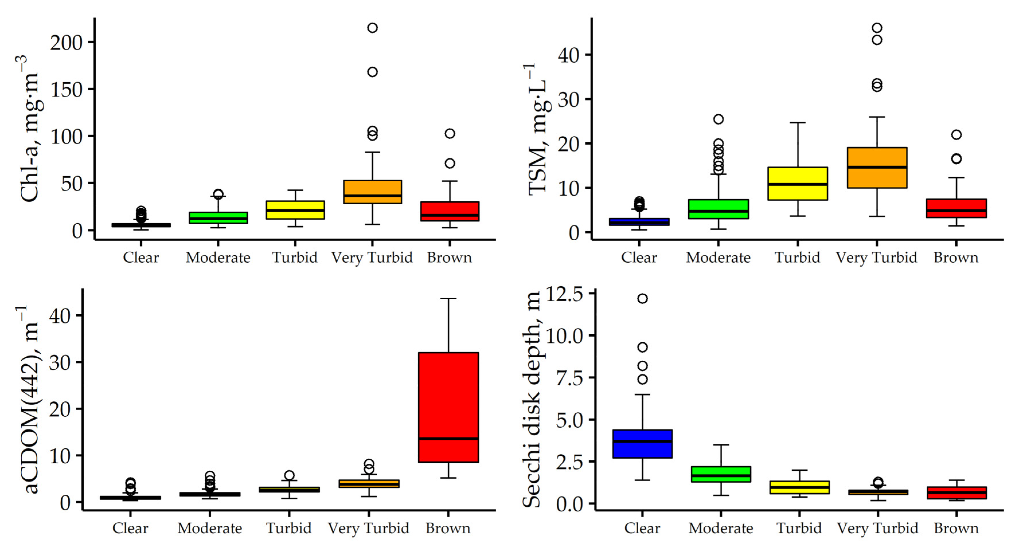
Figure 1. Locations of the in situ measurement stations. Measurement stations of inland waters are marked with red circles and measurement stations of coastal waters with blue diamonds.
Remotesensing 12 00931 g001
Figure 2. Examples of the colour of water photographed in different Estonian lakes: (a) reddish-brown water in Nohipalo Mustjärv (Secchi disk depth 0.3 m; aCDOM(442) 41.1 m−1); (b) greenish water in Lake Tamula (Secchi disk depth 0.5 m); and (c) highly transparent water in lake Nohipalo Valgjärv (Secchi disk depth 5 m).
Remotesensing 12 00931 g002
Figure 3. In situ measured R(λ) classified into various optical water types by the maximum likelihood of individual spectra to type averages, using the spectral correlation similarity and modified spectral angle similarity.
Remotesensing 12 00931 g003
Figure 4. The range of the variation of the concentrations of optically significant constituents, such as chlorophyll-a (Chl-a), total suspended matter (TSM), absorption coefficient of coloured dissolved organic matter at a wavelength of 442 nm (aCDOM(442)), and Secchi disk depth by optical water types.
Remotesensing 12 00931 g004
Figure 5. The accuracy of the optical water type (OWT) assignment using in situ measurements of R(λ) convolved into Ocean and Land Colour Instrument (OLCI) and Multispectral Imager (MSI) bands by normalized confusion matrices. The rows show the true OWTs determined from in situ measurements of R(λ) using Ramses, and the columns show the predicted OWTs determined from the convolved R(λ). The diagonal elements represent the situation where the predicted OWT is the same as the true OWT (i.e., the correct classification).
Remotesensing 12 00931 g005
Figure 6. Comparison of concentrations of Chl-a estimated from in situ measured R(λ) spectra using the optical water type (OWT) guided approach and in situ measured concentrations of Chl-a for different spectral scales: (left to right) Ramses with 1 nm resolution, OLCI, and MSI. OWTs are indicated by colours and the line shows 1:1 relationship.
Remotesensing 12 00931 g006
Figure 7. Comparison of concentrations of TSM estimated from in situ measured reflectance spectra using the optical water type (OWT) guided approach and in situ measured concentrations of TSM for sensors with different spectral scales: (from left) Ramses with 1 nm resolution, OLCI, and MSI. OWTs are indicated by colours and the line shows 1:1 relationship.
Remotesensing 12 00931 g007
Figure 8. Comparison of the absorption coefficients of coloured dissolved organic matter (CDOM) at a wavelength of 442 nm estimated from the in situ measured reflectance spectra using the optical water type (OWT) guided approach and in situ measured absorption coefficients of CDOM at a wavelength of 442 nm, for sensors with different spectral scales: (from left) Ramses with 1 nm resolution, OLCI, and MSI. OWTs are indicated by colours and the line shows a 1:1 relationship.
Remotesensing 12 00931 g008
Figure 9. Comparison of the Secchi disk depth estimated from in situ measured reflectance spectra using the optical water type (OWT) guided approach and in situ measured Secchi disk depth for sensors with different spectral scales: (from left) Ramses with 1 nm resolution, OLCI, and MSI. OWTs are indicated by colours and the line shows a 1:1 relationship.
Remotesensing 12 00931 g009
Figure 10. Changing the optical water types (OWTs) and optical water quality parameters (such as the Chl-a, TSM, CDOM, and Secchi disk depth) before and after a strong wind (day average wind speed 11.2 m·s−1 and the gust over 21 m·s−1) event on 22 June 2018 in Pärnu Bay captured by OLCI images processed with the C2RCC AC processor. Water quality parameters are estimated from R(λ) using OWT based algorithms.
Remotesensing 12 00931 g010
Table 1. Descriptive statistics of the measured in situ optical water quality parameters.
ParameterNo. of StationsMeanMedianRangeSkewness
Chl-a 141519.013.60.5–215.24.3
TSM 24157.65.70.6–46.01.9
aCDOM(442) 34153.92.00.4–43.74.1
Secchi depth, m4111.81.40.2–12.22.1
1 Concentration of chlorophyll a, mg·m−3. 2 Concentration of total suspended matter, mg·L−1. 3 Absorption coefficient of coloured dissolved organic matter at a wavelength of 442 nm, m−1.

