Abstract
Glossy buckthorn (Frangula alnus Mill.) is an alien species in Canada that is invading many forested areas. Glossy buckthorn has impacts on the biodiversity and productivity of invaded forests. Currently, we do not know much about the species’ ecology and no thorough study of its distribution in temperate forests has been performed yet. As is often the case with invasive plant species, the phenology of glossy buckthorn differs from that of other indigenous plant species found in invaded communities. In the forests of eastern Canada, the main phenological difference is a delay in the shedding of glossy buckthorn leaves, which occurs later in the fall than for other indigenous tree species found in that region. Therefore, our objective was to use that phenological characteristic to map the spatial distribution of glossy buckthorn over a portion of southern Québec, Canada, using remote sensing-based approaches. We achieved this by applying a linear temporal unmixing model to a time series of the normalized difference vegetation index (NDVI) derived from Landsat 8 Operational Land Imager (OLI) images to create a map of the probability of the occurrence of glossy buckthorn for the study area. The map resulting from the temporal unmixing model shows an agreement of 69% with field estimates of glossy buckthorn occurrence measured in 121 plots distributed over the study area. Glossy buckthorn mapping accuracy was limited by evergreen species and by the spectral and spatial resolution of the Landsat 8 OLI.
1. Introduction
Biological invasions by alien species can alter biodiversity and ecosystem functioning [1], with potential negative consequences on ecosystem services as well as on agricultural and forest resources [2]. The impacts of alien plants are observed at the species, community, and ecosystem levels [3]; for example, exotic species can modify soil microbial communities, reduce plant diversity, and affect the water and nutrient availability or fire cycles [4,5].
Glossy buckthorn (Frangula alnus Mill., syn. Rhamnus frangula L.) is an alien plant species native to Europe [6], Asia, and North Africa [7]. It was introduced in the United States of America in the 19th century, likely for horticultural purposes [8]. Later found in Ottawa and in southern Ontario in Canada [9], glossy buckthorn continued to spread easterly in the early 20th century and is now common in Québec, New Brunswick, and Nova Scotia [10]. Glossy buckthorn impedes the establishment and growth of valuable native tree species [11,12] and reduces indigenous plant diversity [13]. Although glossy buckthorn is considered a significant threat to ecosystem integrity and forest productivity in Québec [14], a detailed knowledge of its spatial distribution is still lacking and relies mainly on the occurrence of this species in various herbaria. Such knowledge is required to adequately monitor its rate of spread, understand the anthropogenic, environmental, and climatic factors that promote site invasion and, ultimately, to design effective mitigation strategies [15].
Remote sensing techniques have been developed and applied to detect, map, monitor, and characterize invasive plant species in various environments [16,17,18,19]. For example, van Lier et al. [20] have combined high and medium-resolution satellite imagery to map invasive ericaceous shrub distribution in the boreal forest ecosystems of Québec. However, distinguishing alien target species from indigenous vegetation can be challenging due to the mixing of spectral signatures [21]. The use of hyperspectral [22] or multispectral [23] remote sensing images to characterize plant phenological stages may help to discriminate alien from native plant species in the vegetation matrix. Invasive alien plant species often have phenological onset dates (e.g., the bud burst, start, and end of the green up period, flowering, leaf senescence) that differ from those of most native plants in the invaded communities [24,25,26]. These phenological differences result in identifiable features or anomalies in remote sensing-based phenological trajectories of pixels invaded by alien plants relative to those containing native plants only. Anomalies in phenological trajectories can be used to detect target alien species using time-series of remotely sensed images, thus increasing our ability to assess their occurrence and evaluate their extent across the landscape [27]. Although spaceborne moderate spatial resolution multispectral sensors such as Sentinel-2A and Landsat 8 Operational Land Imager (OLI) provide a limited number of bands compared to hyperspectral sensors, such as EO-1 Hyperion, they offer frequent and easily accessible images that can be combined with invasive species phenological characteristics to map their occurrence and coverage [27,28,29,30,31,32].
In this context, our objective was to develop an approach to map the occurrence of glossy buckthorn in a region of southern Québec using a time series of a phenology indicator derived from free and readily available multispectral satellite data. We tested the hypothesis that glossy buckthorn phenological trajectory, monitored using the normalized difference vegetation index (NDVI) [33], allows one to discriminate glossy buckthorn from other co-occurring plant species. To achieve this, we derived plot-level vegetation NDVI trajectories from time series of Landsat 8 OLI images and used them as inputs to a linear temporal unmixing procedure. Endmember fractions from unmixing the NDVI stack were used to map the probability of occurrence of glossy buckthorn over our study region.
2. Methods
2.1. Study Area
The study area was located in southern Québec, Canada (45°33′17″N, 71°53′05″W) (Figure 1A), in the sugar maple (Acer saccharum Marsh.)-basswood (Tilia americana L.) bioclimatic domain [34]. The study area was divided into two zones, hereafter referred to as Richmond and Cookshire. Over the last 50 years, monthly mean temperature and monthly mean precipitation in the study area ranged from −6.2 to 18.6°C and 96.3 to 165.4 mm, respectively [35]. Most of the study area was covered by forest stands (75%) that were distributed among the following cover types: broadleaf deciduous (36%), mixedwood (34%), evergreen needleleaf (17%), and regenerating stands (13%) [36]. Forest stands in the Richmond zone were mainly composed of broadleaf deciduous forest tree species, such as Betula alleghaniensis Britt., Acer rubrum L., Acer saccharum, and Fagus grandifolia Ehrh. The Cookshire zone was dominated by coniferous stands containing species such as Abies balsamea L., Pinus resinosa Ait., and Pinus strobus L. In both zones, soils were dominated by poorly to well drained brunisols (occasionally podzols) that developed on top of undifferentiated till (Soil Classification Working Group 1998). The humus was generally acidic and was characterized by a slow mineralization process (moder).
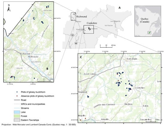
Figure 1.
Study area (A) showing the two zones (B: Richmond; C: Cookshire). The black rectangle in the upper right inset shows the location of the study area in southern Québec, Canada.
2.2. Field Sampling
During the summer of 2015, we assessed glossy buckthorn cover in 124 sample plots (30 × 30 m) distributed over 45 private forest lots of the Richmond and Cookshire zones. A selection of candidate forest stands for field sampling was made based on information on glossy buckthorn history and cover obtained from the agency responsible for managing private forest land in the study region. Two criteria were used for identifying candidate stands: firstly, glossy buckthorn had to cover at least 900 m2 of the stand total area and, secondly, observations of its presence in the stand needed to go back to at least three years prior to field sampling. These criteria ensured coherence between field measurements and Landsat 8 images and also increased the likelihood of detecting glossy buckthorn in 30 × 30 m pixels. From the set of candidate stands, we made the final selection with the objective of sampling the widest possible range in glossy buckthorn cover, forest cover types, site conditions (e.g., soil drainage, surficial deposit), and stand attributes. Site conditions and stand attributes (e.g., cover type, crown cover) were extracted from a 1:20 k provincial forest map [37]. We also aimed at maximizing the spatial distribution of the plots over the study area. We anticipated that evergreen foliage would reduce our capacity to isolate glossy buckthorn phenological characteristics from those of coniferous trees. For this reason, we tried to limit the number of plots in forest stands dominated by coniferous tree species. Finally, all plots were located at least 50 m from each other or from any spectrally contrasting feature, such as roads and clear-cuts, to reduce potential edge effects on OLI reflectance values [38].
We assessed plot-level glossy buckthorn cover using a modified version of the point-intercept method [39]. Plots were measured between May 12 and June 6 of 2015. In each plot, we established three 30-m long transects that were spaced 10 m apart and oriented north-south. Along each transect, we established one 4 m2-circular subplot (diameter = 1.13 m) every 5 m (7 subplots/transect), in which we assessed the occurrence of glossy buckthorn (presence/absence) and of other tree or shrub species in the subplot. Plot-level glossy buckthorn cover (%) was then calculated as the ratio of the number of subplots containing glossy buckthorn to the total number of subplots (N = 21). All sampled plots were geolocated using a Garmin Oregon 650 GPS (the Horizontal Dilution of Precision (HDOP) under the forest canopy was below 6 m using the Wide Area Augmentation System, or WAAS).
2.3. Processing of Landsat-8 OLI Images
We downloaded a time series of Landsat 8 OLI images (L1T) encompassing our study area from the USGS Global Visualization Viewer (GloVis) website (https://glovis.usgs.gov/). We limited our time series to images acquired between April and November during the years 2013 to 2015 and rejected images with a cloud cover above 10% (Table 1). Differences in atmospheric conditions between images in the time series can reduce the performance of change detection algorithms [40,41]. To minimize this source of noise, we used the ATCOR Ground Reflectance module in PCI Geomatica [42] to transform OLI digital numbers (DN) into surface reflectance values. Standard continental atmospheric properties and rural aerosol conditions were assumed, and vegetation was considered as a Lambertian surface. Topographic effects were also corrected in ATCOR using the Canadian Digital Elevation Model [43]. Finally, we extracted surface reflectance values in OLI 30 m bands 4 (red, 0.64–0.67 µm) and 5 (near-infrared, 0.85–0.88 µm) for all forest pixels in the time series. We masked non-forested pixels using the 1:20 k provincial forest maps.

Table 1.
Landsat 8 Operational Land Imager (OLI) images used in this study. All images were acquired along path 13 and row 28 (WRS-2) in descending mode.
2.4. NDVI Times Series
To identify the best temporal window for predicting glossy buckthorn occurrence and to obtain input and validation data for the phenology-based unmixing procedure, we calculated the NDVI for each date of OLI acquisition as:
where ρi is the surface reflectance in OLI band i. We generated NDVI time series for each measured plot by averaging, for each date, the NDVI values from a 3 × 3 pixel window centered on each plot coordinate. Finally, plot-level NDVI time series were used, along with glossy buckthorn percent cover measured in field plots, to determine the minimum cover value at which glossy buckthorn cover could be detected using the temporal unmixing approach.
2.5. Temporal Unmixing
The high level of spatial heterogeneity of forested areas, combined with the moderate spatial resolution of OLI, resulted in spectrally mixed forest pixels. To disentangle glossy buckthorn signals in mixed pixels, we used a linear spectral unmixing approach [44]. We applied spectral unmixing in the temporal domain, replacing spectral bands with image dates to retrieve the relative abundance (i.e., fraction) of cover types inside image pixels. Linear spectral mixture models consider pixel reflectance as a weighted sum of homogeneous spectral components called endmembers. Thus, we chose three temporally distinct endmembers (cover types), which also exhibit marked differences in their phenological trajectories: deciduous, coniferous, and glossy buckthorn. To create endmembers’ temporal signatures, we used percent cover data measured in field plots. For each endmember, we selected one plot in which endmember cover type was at least 70% of the plot area. Field plots used for endmember selection were excluded from subsequent analyses. Endmember percentage cover values were 89%, 70%, and 80% for glossy buckthorn, deciduous, and coniferous endmembers, respectively. To minimize the influence of soil and background vegetation on endmember NDVI values, deciduous and coniferous endmember plots were selected among dense forest stands in which glossy buckthorn was absent. The glossy buckthorn endmember plot was located in a stand where tree cover was absent and that had the highest glossy buckthorn cover of all measured plots. To ensure a well-closed canopy, we used a summer NDVI image (August 19, 2015) to delineate, for each endmember, a group of contiguous pixels from the plot center. Endmember pixels were then extracted from each NDVI image and their descriptive statistics (minimum, maximum, mean, standard deviation) were extracted, by endmember and by date, to be used as inputs to the linear unmixing procedure. We used a t-test to confirm phenological differences between each endmember, which suggested that plots invaded by glossy buckthorn and those from which it was absent could be temporally distinguished. To account for the multiplicity of the test at each date (N = 3), we used the Bonferroni correction and used a threshold of 0.017 (0.05/3) to consider differences as significant (see Appendix A).
A linear spectral mixture model was created in the ENVI 4.8 software [45] and applied to unmix the time series of NDVI images. This model was used to assess the fraction of each endmember at the forested pixel level. The mixture model used in this procedure assumed that the NDVI time series results from each endmember. We used a fraction value of 0.4 to determine if a pixel was invaded by glossy buckthorn or not. This fraction was determined using a combination of the receiver operating characteristic (ROC) and Pareto front. The ROC curve was used to evaluate the effect of different fraction values on the false negative and true positive rates. We then used a Pareto front to determine the threshold fraction that allowed to minimize false negative rate while also maximizing the true positive rate (see Appendix B). The classification accuracy was evaluated using data from the remaining 121 field plots (109 invaded and 12 non-invaded). We used confusion matrices to calculate omission (lack of predictions) and commission (excess of predictions) errors and the level of agreement (accuracy) between field observations and model predictions.
3. Results
3.1. Field-Based Measurements of Glossy Buckthorn Cover
The average glossy buckthorn cover from all field plots was 62.6%, with minimum and maximum values of 0% and 89%, respectively (Table 2). Glossy buckthorn cover differed significantly between the two zones, with higher values in Cookshire than in Richmond (65.3% vs. 57.9%, respectively; p = 0.008).
Table 2.
Descriptive statistics of glossy buckthorn cover and tree canopy cover from plots measured in Richmond and Cookshire.
3.2. Validation of the Phenology-Based Map of Glossy Buckthorn Occurrence
Glossy buckthorn was detected in only two of the 21 plots dominated by conifer trees, suggesting that dense conifer canopies may be an obstacle to the accurate detection of glossy buckthorn, regardless of the time of year. Therefore, coniferous-dominated plots were excluded, which left 100 plots from subsequent validation analyses. The confusion matrix (Table 3) shows that the classification method achieved a global accuracy of 69%, meaning that 69% of present glossy buckthorn was classified accurately (true positive rate = 62/90). Similarly, 70% of the sites in which glossy buckthorn was absent were correctly classified. On the other hand, our approach could not detect glossy buckthorn presence in 31% of the plots where it was present (false negative rate = 28/90), whereas in 30% of the cases its presence was predicted when it was actually absent from the plot (false positive rate = 3/10).
Table 3.
Confusion matrix for glossy buckthorn occurrence estimated from temporal linear unmixing of the Landsat-8 OLI normalized difference vegetation index (NDVI) image series. The threshold value (% cover) was used to determine if glossy buckthorn was present if the endmember fraction map was set to 0.4 (minimum glossy buckthorn cover measured value in presence plots was 27%).
The important variability in glossy buckthorn percent cover among the 90 plots where it was found allowed splitting the dataset into three cover classes. The classification performance increased as the class lower bound increased, with an 11% increase from the class covering the largest range in buckthorn cover (≥25%) to that containing only plots with a high buckthorn cover (≥75%) (Table 4).
Table 4.
Agreement and disagreement values calculated from the confusion matrices of different glossy buckthorn cover classes. Each confusion matrix used the same amount of absence plots (N = 10) but decreasing numbers of presence plots (≥ 25%: N = 90 (lowest glossy buckthorn cover), ≥65%: N = 60 (average glossy buckthorn cover), ≥ 75%: N = 32).
Given the differences in forest cover between the two zones (Table 2), we compared the performance of our classifier by calculating agreement/disagreement values separately for each zone. We found a marked difference in performance between Richmond (59% agreement) and Cookshire (75% agreement). Figure 2 shows commission and omission errors and the agreement between predictions and observation data. Omission errors were more frequent in the presence (30%) than in the absence classes (8%). Commission errors comprised most of the prediction errors in the absence class (75%), indicating an over-representation of pixels free of glossy buckthorn in the resulting map.
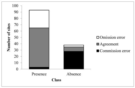
Figure 2.
Omission and commission errors and agreement between predictions of glossy buckthorn occurrence from the phenology-based method and measurements from 100 plots (the number of validation plots (100) that correspond to the sum of gray and white only).
In most forested areas of the Richmond zone, glossy buckthorn was identified by temporal unmixing analysis. There were some places where the probability of occurrence of glossy buckthorn was more than 90% (Figure 3).
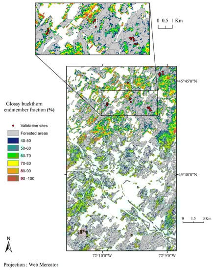
Figure 3.
Glossy buckthorn endmember fraction (%) in mixed and deciduous forest stands of the Richmond zone estimated from the linear temporal unmixing of a Landsat 8 NDVI time series (2013–2015).
The results show a different pattern for the Cookshire zone (Figure 4). Indeed, glossy buckthorn was present but scattered in the landscape. There was some forested area where glossy buckthorn was likely absent.
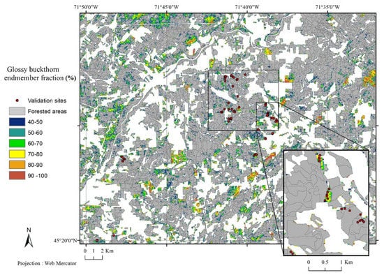
Figure 4.
Glossy buckthorn endmember fraction (%) in mixed and deciduous forest stands of the Cookshire zone estimated from linear unmixing of a Landsat 8 NDVI time series (2013–2015).
4. Discussion
An earlier study using Landsat-7 ETM+ data suggested that glossy buckthorn should compose at least 70% of the canopy in pixels to be successfully identified [46]. Likewise, we found that the mapping of buckthorn occurrence was more accurate in plots where glossy buckthorn cover was higher than 70%. High spatial resolution hyperspectral or multispectral images would have been a better tool than Landsat imagery for investigating zones where glossy buckthorn covered less than 70% of the canopy. However, the costs associated with high spatial resolution images (<1 m/pixel) are high and they generally require advanced processing methods and a high computing power [47]. Becker et al. [46] mapped glossy buckthorn and common buckthorn (Rhamnus cathartica L.) in a territory using 50 × 50 m experimental plots. Unfortunately, their classification with Landsat 5 TM and Landsat 7 ETM + was found to be ineffective in patches smaller than 50 × 50 m. Most of our field plots showed a dense 2–3-m high glossy buckthorn cover. We commonly encountered dispersed small patches of dense glossy buckthorn bushes, which were undoubtedly difficult to identify using 30-m Landsat 8 OLI images. It is likely that this particularity, combined with a well-developed tree cover, has contributed to the high false negative rate we obtained and that this would limit the precision of this approach if applied for mapping glossy buckthorn occurrence in stands where similar attributes exist. Our mapping was cautious because it included only places heavily invaded by glossy buckthorn and can be used as a reference map for future analysis. The high commission error rate reveals that the model failed to predict the absence of glossy buckthorn in the study area. Indeed, the model underestimated the actual invasion of glossy buckthorn in most coniferous stands. This underestimation is particularly important since conifers occupy 17% of the study area. Therefore, it appears that multispectral optical remote sensing data such as Landsat 8 OLI is not the optimal tool for mapping glossy buckthorn occurrence in these stands since these plants remain invisible to the instrument throughout the year under dense conifer canopies. This limitation might become more important in the coming decades, as climate change will potentially favor the extension of glossy buckthorn distribution in the Canadian boreal forest (from where is it actually relatively absent).
There were several reasons why our mapping was more effective in Cookshire than in the Richmond zone. First, field observations by managers and foresters showed that the invasion was extensive in Cookshire. This may also be explained by the difference in stand cover of the validation sites, which was lower in Cookshire than in Richmond. For sure, it was more difficult to identify glossy buckthorn through a dense forest canopy, even knowing that the leaves have fallen at some point, due to the interference caused by the presence of branches and tree trunks. By comparison, a study using a time series of NDVI to perform the characterization of glossy buckthorn and common buckthorn, managed to successfully identify these two species in Ohio and Michigan (USA) with a kappa of 0.73 [46]. This seems greatly facilitated by the ecological characteristics of the study area, since communities were mainly oak grasslands, low-cover environments without conifer species. Our results suggest that phenology-based mapping using unmixing and the time series of multispectral satellite data may be more efficient to detect species at a lower threshold than traditional approaches.
Along with complications due to the tree canopy, there were also other interferences, such as the presence of exposed soil and of other plant species, such as ferns (primarily Onoclea sensibilis L.) or speckled alder (Alnus rugosa (Du Roi) Spreng.). Speckled alder is a shrub that grows in the understory, very similar to glossy buckthorn, also considered a companion species of the latter. The presence of this understory vegetation modified the reflectance signal of the canopy. According to some authors, these variations can be over 18% in the red band, and over 10% in the infrared band [48]. Some studies have even used this variability in the reflectance values to detect the type of understory vegetation [49,50,51]. Using Landsat 8 (OLI) allowed the classification of an invaded forest according to forest types, rather than the understory species themselves. The spatial resolution of Landsat 8 sensor (OLI) thus represents a limit when trying to map smaller entities than the pixel.
Other images with a higher spatial or spectral resolution (such as WorldView, IKONOS, Quickbird) could have been used in this study, but the costs associated with these images are prohibitive and, moreover, they may not be available for the desired dates and regions of interest. This is also the case for airborne (AVIRIS, CASI, etc.) or in-orbit (EO1-Hyperion) hyperspectral imagery. Hyperspectral sensors could greatly improve glossy buckthorn mapping because of their ability to discriminate pixels by taking advantage of the richness of the spectral information contained in large numbers of high-spectral resolution bands [52]. In addition, it is sometimes necessary to make several corrections to obtain images without blur, which complicates the use of these images [53]. Although they have proved to be efficient in mapping alien species, e.g., [54], the acquisition of these images by airborne sensors can be complex with respect to the availability of flying machines or current regulations [27]. LiDAR was used for classifying understory species in coniferous stands [55,56]. This tool could also improve outcomes for mapping glossy buckthorn, since the tool is able to provide information from under the tree canopy. Because the structure of coniferous stands differs from that of deciduous forests [57], and also because it can be modified by the presence of an alien invasive species in the understory [58], it is likely that the presence of glossy buckthorn in coniferous woods can be detected with LiDAR. In addition, the amount of commission errors in the absence class indicates that more invaded pixels were not properly classified as a presence, reflected again by an underestimation of the cover.
5. Conclusions
Temporal unmixing performed on a time series of Landsat8 (OLI) NDVI images allowed for the detection of glossy buckthorn in deciduous and mixed forest. The mapping allowed to identify forest stands heavily overgrown by glossy buckthorn, but did not allow detection in coniferous stands. Thus, the study helped to partially verify the hypothesis that phenology allows to discriminate the temporal signature of glossy buckthorn from that of other forest cover types found in the study area. In order to improve the occurrence mapping of glossy buckthorn, other avenues should be considered such as increasing the number of presence and absence sites to better reflect the great variability in forest structures and compositions (cover types, canopy closure, settlement patterns, etc.). This would allow for the selection of more representative points of absence for the calculation of homogeneous spectral components. Other spectral indices less likely to saturate in well-developed biomass stands (e.g., EVI or ARVI) could improve the glossy buckthorn detection threshold.
Author Contributions
Conceptualization, J.L., G.D., J.-D.S., N.T., F.H. and F.G.; methodology and formal analysis, J.L., G.D., J.-D.S. and F.G.; supervision, F.G. and F.H.; writing—original draft preparation, J.L.; writing—review and editing, G.D., J.-D.S., N.T., F.H. and F.G. All authors have read and agreed to the published version of the manuscript.
Funding
Funding was provided by the Agence de mise en valeur de la forêt privée de l’Estrie, the Natural Sciences and Engineering Research Council of Canada (NSERC), the Fonds de recherche - Nature et Technologie, in collaboration with the Direction de la recherche forestière, Ministère des Forêts, de la Faune et des Parcs du Québec and the Canadian Wood Fibre Centre.
Acknowledgments
We are thankful to Mario Dionne, Marie-Josée Martel, Jean Tremblay, James Kerr, Yves Harnois, Ken Dubé, Lise Beauséjour and Isabelle Simard for their contribution to the project. We thank the anonymous reviewers who provided constructive comments on an earlier version of this work.
Conflicts of Interest
The authors declare no conflict of interest.
Appendix A

Figure A1.
Landsat 8 OLI-derived NDVI phenological trajectories (i.e., temporal spectra) for the endmembers used in the unmixing procedure. Data points are mean NDVI values for groups of pixels extracted around each endmember field plot and for each image acquisition date. The error bars represent standard deviation for the same dates and groups of points.
Table A1.
Comparisons of endmember mean values: t-tests F-stats and P-values for each pair of endmember and the date of image acquisition. P-values in bold indicate a significant difference in mean between two groups for a given date. To account for the multiplicity of the test at each date (N = 3), we applied the Bonferroni correction. P-values below 0.017 (0.05/3) were considered as significant.
| Treatement | ||||||
|---|---|---|---|---|---|---|
| Deciduous vs Glossy Buck. | Deciduous vs Coniferous | Coniferous vs Glossy Buck. | ||||
| Day of year | F-Stats | P-Value | F-Stats | P-Value | F-Stats | P-Value |
| 113 | −7.1 | 0.000 | −5.2 | 0.002 | −14.5 | 0.004 |
| 161 | −4.4 | 0.001 | 3.0 | 0.086 | 1.8 | 0.198 |
| 231 | 12.4 | 0.000 | 0.3 | 0.808 | 6.5 | 0.011 |
| 273 | 28.4 | 0.000 | −3.3 | 0.016 | 25.9 | 0.000 |
| 276 | 13.7 | 0.000 | −7.2 | 0.000 | 8.1 | 0.000 |
| 327 | −4.9 | 0.001 | −5.2 | 0.008 | −9.2 | 0.010 |
Appendix B

Figure A2.
The ROC curve used to determine the optimal threshold value for predicting the occurrence of glossy buckthorn. A Pareto front was used to determine the fraction of glossy buckthorn that allows one to minimize the false negative rate and maximize the true positive rate. The black line describes the behavior of the ROC algorithm for all possible threshold values, while the blue dashed line represents a random classifier with no power of discrimination.
References
- Tylianakis, J.M.; Didham, R.K.; Bascompte, J.; Wardle, D.A. Global change and species interactions in terrestrial ecosystems. Ecol. Lett. 2008, 11, 1351–1363. [Google Scholar] [CrossRef]
- Mack, R.N.; Simberloff, D.; Mark Lonsdale, W.; Evans, H.; Clout, M.; Bazzaz, F.A. Biotic invasions: Causes, epidemiology, global consequences, and control. Ecol. Appl. 2000, 10, 689–710. [Google Scholar] [CrossRef]
- Vilà, M.; Espinar, J.L.; Hejda, M.; Hulme, P.E.; Jarošík, V.; Maron, J.L.; Pergl, J.; Schaffner, U.; Sun, Y.; Pyšek, P. Ecological impacts of invasive alien plants: A meta-analysis of their effects on species, communities and ecosystems. Ecol. Lett. 2011, 14, 702–708. [Google Scholar] [CrossRef]
- Knight, K.S.; Kurylo, J.S.; Endress, A.G.; Stewart, J.R.; Reich, P.B. Ecology and ecosystem impacts of common buckthorn (Rhamnus cathartica): A review. Biol. Invasions 2007, 9, 925–937. [Google Scholar] [CrossRef]
- Krumm, F.; Vítková, L. Introduced Tree Species in European Forests: Opportunities and Challenges; European Forest Institute: Berlin, Germany, 2016. [Google Scholar]
- Medan, D. Reproductive biology ofFrangula alnus (Rhamnaceae) in southern Spain. Plant Syst. Evol. 1994, 193, 173–186. [Google Scholar] [CrossRef]
- Converse, C.K. Element Stewardship Asbstrat for Rhamnus cathartica, Rhamnus frangula (syn. Frangula alnus); The Nature Conservancy: Arlington, VA, USA, 1984. [Google Scholar]
- Howell, J.A.; Blackwell, W.H., Jr. The history of Rhamnus frangula (glossy buckthorn) in the Ohio flora. Castanea 1977, 42, 111–115. [Google Scholar]
- Catling, P.M.; Porebski, Z.S. The History of Invasion and Current Status of Glossy Buckthorn, Rhamnus-Frangula, in Southern Ontario. Can. Field-Nat. 1994, 108, 305–310. [Google Scholar]
- Haber, E. Spread and impact of alien plants across Canadian landscapes. In Alien Invaders in Canada’s Waters, Wetlands and Forests; Canadian Forest Service: Ottawa, ON, Canada, 2002; pp. 43–57. [Google Scholar]
- Fagan, M.E.; Peart, D.R. Impact of the invasive shrub glossy buckthorn (Rhamnus frangula L.) on juvenile recruitment by canopy trees. For. Ecol. Manag. 2004, 194, 95–107. [Google Scholar] [CrossRef]
- Hamelin, C.; Truax, B.; Gagnon, D. Invasive glossy buckthorn impedes growth of red oak and sugar maple under-planted in a mature hybrid poplar plantation. New For. 2016, 47, 897–911. [Google Scholar] [CrossRef]
- Frappier, B.; Eckert, R.T.; Lee, T.D. Experimental removal of the non-indigenous shrub Rhamnus frangula (glossy buckthorn): Effects on native herbs and woody seedlings. Northeast. Nat. 2004, 11, 333–342. [Google Scholar] [CrossRef]
- Beaudet, M.; Cauboue, M.; Thiffault, N.; Cartier, P.; Martineau, P.; Boulet, B. L’autécologie des especes concurrentes. In Le Guide Sylvicole du Québec; Les publications du Québec: Québec, QC, Canada, 2013; Volume 1, pp. 180–279. [Google Scholar]
- Kerr, J.T.; Ostrovsky, M. From space to species: Ecological applications for remote sensing. Trends Ecol. Evol. 2003, 18, 299–305. [Google Scholar] [CrossRef]
- Madden, M. Remote Sensing and Geographic Information System Operations for Vegetation Mapping of Invasive Exotics. Weed Technol. 2004, 18, 1457–1463. [Google Scholar] [CrossRef]
- Wang, N. Application of Remote Sensing in Detecting and Monitoring Forest Regeneration Process in a Disturbed Environment. M.Sc. Thesis, Carleton University, Ottawa, ON, Canada, 1995. [Google Scholar]
- Zweig, C.L.; Newman, S. Using landscape context to map invasive species with medium-resolution satellite imagery. Restor. Ecol. 2015, 23, 524–530. [Google Scholar] [CrossRef]
- Frazier, A.E.; Wang, L. Characterizing spatial patterns of invasive species using sub-pixel classifications. Remote Sens. Environ. 2011, 115, 1997–2007. [Google Scholar] [CrossRef]
- Van Lier, O.R.; Fournier, R.A.; Bradley, R.L.; Thiffault, N. A multi-resolution satellite imagery approach for large area mapping of ericaceous shrubs in Northern Quebec, Canada. Int. J. Appl. Earth Obs. Geoinf. 2009, 11, 334–343. [Google Scholar] [CrossRef]
- Miao, X.; Gong, P.; Swope, S.; Pu, R.; Carruthers, R.; Anderson, G.L. Detection of yellow starthistle through band selection and feature extraction from hyperspectral imagery. Photogramm. Eng. Remote Sens. 2007, 73, 1005. [Google Scholar]
- Andrew, M.E.; Ustin, S.L. The role of environmental context in mapping invasive plants with hyperspectral image data. Remote Sens. Environ. 2008, 112, 4301–4317. [Google Scholar] [CrossRef]
- Tuanmu, M.-N.; Viña, A.; Bearer, S.; Xu, W.; Ouyang, Z.; Zhang, H.; Liu, J. Mapping understory vegetation using phenological characteristics derived from remotely sensed data. Remote Sens. Environ. 2010, 114, 1833–1844. [Google Scholar] [CrossRef]
- Xu, C.-Y.; Griffin, K.L.; Schuster, W. Leaf phenology and seasonal variation of photosynthesis of invasive Berberis thunbergii (Japanese barberry) and two co-occurring native understory shrubs in a northeastern United States deciduous forest. Oecologia 2007, 154, 11–21. [Google Scholar] [CrossRef]
- Fridley, J.D. Extended leaf phenology and the autumn niche in deciduous forest invasions. Nature 2012, 485, 359. [Google Scholar] [CrossRef]
- Polgar, C.; Gallinat, A.; Primack, R.B. Drivers of leaf-out phenology and their implications for species invasions: Insights from Thoreau’s Concord. New Phytol. 2014, 202, 106–115. [Google Scholar] [CrossRef] [PubMed]
- Huang, C.Y.; Asner, G.P. Applications of remote sensing to alien invasive plant studies. Sensors 2009, 9, 4869–4889. [Google Scholar] [CrossRef] [PubMed]
- Peterson, E. Estimating cover of an invasive grass (Bromus tectorum) using tobit regression and phenology derived from two dates of Landsat ETM + data. Int. J. Remote Sens. 2005, 26, 2491–2507. [Google Scholar] [CrossRef]
- Resasco, J.; Hale, A.; Henry, M.; Gorchov, D. Detecting an invasive shrub in a deciduous forest understory using late-fall Landsat sensor imagery. Int. J. Remote Sens. 2007, 28, 3739–3745. [Google Scholar] [CrossRef]
- Shiferaw, H.; Schaffner, U.; Bewket, W.; Alamirew, T.; Zeleke, G.; Teketay, D.; Eckert, S. Modelling the current fractional cover of an invasive alien plant and drivers of its invasion in a dryland ecosystem. Sci. Rep. 2019, 1. [Google Scholar] [CrossRef] [PubMed]
- Radoux, J.; Chomé, G.; Jacques, D.C.; Waldner, F.; Bellemans, N.; Matton, N.; Lamarche, C.; D’Andrimont, R.; Defourny, P. Sentinel-2’s Potential for Sub-Pixel Landscape Feature Detection. Remote Sens. 2016, 8, 488. [Google Scholar] [CrossRef]
- Müllerová, J.; Brůna, J.; Bartaloš, T.; Dvořák, P.; Vítková, M.; Pyšek, P. Timing is important: Unmanned aircraft vs. satellite imagery in plant invasion monitoring. Front. Plant Sci. 2017, 8, 887. [Google Scholar] [CrossRef]
- Tucker, C.J. Red and photographic infrared linear combinations for monitoring vegetation. Remote Sens. Environ. 1979, 8, 127–150. [Google Scholar] [CrossRef]
- Saucier, J.-P.; Robitaille, A.; Grondin, P. Cadre bioclimatique du Québec. In Écologie Forestière—Manuel de Foresterie, 2nd ed.; Doucet, R., Côté, M., Eds.; Ordre des ingénieurs forestiers du Québec: Québec, QC, Canada, 2009; pp. 186–205. [Google Scholar]
- Environnement Canada. Normales et Moyennes Climatiques de la Région de l’Estrie; Environnement Canada: Ottawa, ON, Canada, 2016.
- Laliberté, F.; Gauthier, J.; Boileau, J.F.; Chauvette, B. Portrait de la Forêt Naturelle et des Enjeux Écologiques de l’Estrie. Master’s Thesis, Université de Montréal, Montreal, QC, Canada, 2015; 114p. [Google Scholar]
- Ministère des Forêts, de la Faune et des Parcs (MFFP). Norme de Stratification Écoforestière du 4e Inventaire Écoforestier du Québec Méridional; Gouvernement du Québec: Québec, QC, Canada, 2015; 111p. Available online: http://www.mffp.gouv.qc.ca/forets/inventaire/pdf/norme-stratification.pdf (accessed on 3 February 2020).
- Campbell, J.B.; Wynne, R.H. Introduction to Remote Sensing, 5th ed.; The Guilford Press: New York, NY, USA, 2011; 667p. [Google Scholar]
- Mueller-Dombois, D.; Ellenberg, H. Aims and Methods of Vegetation Ecology; John Wiley & Sons: New York, NY, USA, 1974; 547p. [Google Scholar]
- Vicente-Serrano, S.M.; Pérez-Cabello, F.; Lasanta, T. Assessment of radiometric correction techniques in analyzing vegetation variability and change using time series of Landsat images. Remote Sens. Environ. 2008, 112, 3916–3934. [Google Scholar] [CrossRef]
- Song, C.; Woodcock, C.E.; Seto, K.C.; Lenney, M.P.; Macomber, S.A. Classification and change detection using Landsat TM data: When and how to correct atmospheric effects? Remote Sens. Environ. 2001, 75, 230–244. [Google Scholar] [CrossRef]
- Geomatica, version 10; PCI Geomatics: Markham, ON, Canada, 2015.
- Natural Resources Canada. Canadian Digital Elevation Model Product Specifications, Edition 1.1; Government of Canada: Québec, QC, Canada, 2013. Available online: http://ftp.maps.canada.ca/pub/nrcan_rncan/elevation/cdem_mnec/doc/CDEM_product_specs.pdf (accessed on 3 February 2020).
- Adams, J.B.; Gillespie, A.R. Remote Sensing of Landscapes with Spectral Images: A Physical Modeling Approach, 1st ed.; Cambridge University Press: Cambridge, UK, 2006; 378p. [Google Scholar]
- ENVI Image Analysis Software, version 10.1.; Harris Geospatial: Broomfield, CO, USA, 2011.
- Becker, R.H.; Zmijewski, K.A.; Crail, T. Seeing the forest for the invasives: Mapping buckthorn in the Oak Openings. Biol. Invasions 2012, 15, 315–326. [Google Scholar] [CrossRef]
- Xie, Y.; Sha, Z.; Yu, M. Remote sensing imagery in vegetation mapping: A review. J. Plant Ecol. 2008, 1, 9–23. [Google Scholar] [CrossRef]
- Eriksson, H.M.; Eklundh, L.; Kuusk, A.; Nilson, T. Impact of understory vegetation on forest canopy reflectance and remotely sensed LAI estimates. Remote Sens. Environ. 2006, 103, 408–418. [Google Scholar] [CrossRef]
- Kuusk, A.; Lang, M.; Nilson, T. Simulation of the reflectance of ground vegetation in sub-boreal forests. Agric. For. Meteorol. 2004, 126, 33–46. [Google Scholar] [CrossRef]
- Peltoniemi, J.I.; Kaasalainen, S.; Näränen, J.; Rautiainen, M.; Stenberg, P.; Smolander, H.; Smolander, S.; Voipio, P. BRDF measurement of understory vegetation in pine forests: Dwarf shrubs, lichen, and moss. Remote Sens. Environ. 2005, 94, 343–354. [Google Scholar] [CrossRef]
- Rautiainen, M.; Suomalainen, J.; Mõttus, M.; Stenberg, P.; Voipio, P.; Peltoniemi, J.; Manninen, T. Coupling forest canopy and understory reflectance in the Arctic latitudes of Finland. Remote Sens. Environ. 2007, 110, 332–343. [Google Scholar] [CrossRef]
- Dobigeon, N.; Altmann, Y.; Brun, N.; Moussaoui, S. Linear and nonlinear unmixing in hyperspectral imaging. In Resolving Spectral Mixtures—With Application from Ultrafast Spectroscopy to Super-Resolution Imaging; Elsevier: Amsterdam, The Netherlands, 2016; p. 45. [Google Scholar]
- Royimani, L.; Mutanga, O.; Odindi, J.; Dube, T.; Matongera, T.N. Advancements in satellite remote sensing for mapping and monitoring of alien invasive plant species (AIPs). Phys. Chem. Earth 2019, 112, 237–245. [Google Scholar] [CrossRef]
- Andrew, M.E.; Ustin, S.L. Habitat suitability modelling of an invasive plant with advanced remote sensing data. Divers. Distrib. 2009, 15, 627–640. [Google Scholar] [CrossRef]
- Kim, S.; Hinckley, T.; Briggs, D. Classifying tree species using structure and spectral data from LIDAR. In Proceedings of the ASPRS/MAPPS 2009 Specialty Conference, San Antonio, TX, USA, 16–19 November 2009. [Google Scholar]
- Reitberger, J.; Krzystek, P.; Stilla, U. Analysis of full waveform LIDAR data for the classification of deciduous and coniferous trees. Int. J. Remote Sens. 2008, 29, 1407–1431. [Google Scholar] [CrossRef]
- Stenberg, P.; Mottus, M.; Rautiainen, M. Modeling the spectral signature of forests: Application of remote sensing models to coniferous canopies. In Advances in Land Remote Sensing; Springer: Berlin, Germany, 2008; pp. 147–171. [Google Scholar]
- Asner, G.P.; Hughes, R.F.; Vitousek, P.M.; Knapp, D.E.; Kennedy-Bowdoin, T.; Boardman, J.; Martin, R.E.; Eastwood, M.; Green, R.O. Invasive plants transform the three-dimensional structure of rain forests. Proc. Natl. Acad. Sci. USA 2008, 105, 4519–4523. [Google Scholar] [CrossRef]
© 2020 by the authors. Licensee MDPI, Basel, Switzerland. This article is an open access article distributed under the terms and conditions of the Creative Commons Attribution (CC BY) license (http://creativecommons.org/licenses/by/4.0/).