Quantifying Information Content in Multispectral Remote-Sensing Images Based on Image Transforms and Geostatistical Modelling


Abstract
1. Introduction
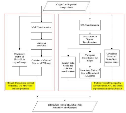
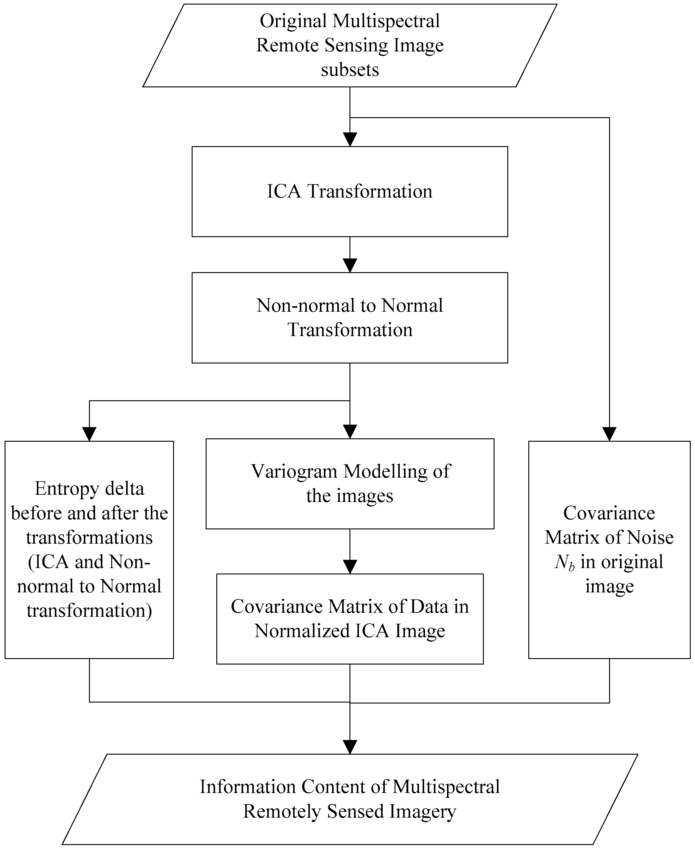
2. Methods
3. Experiments
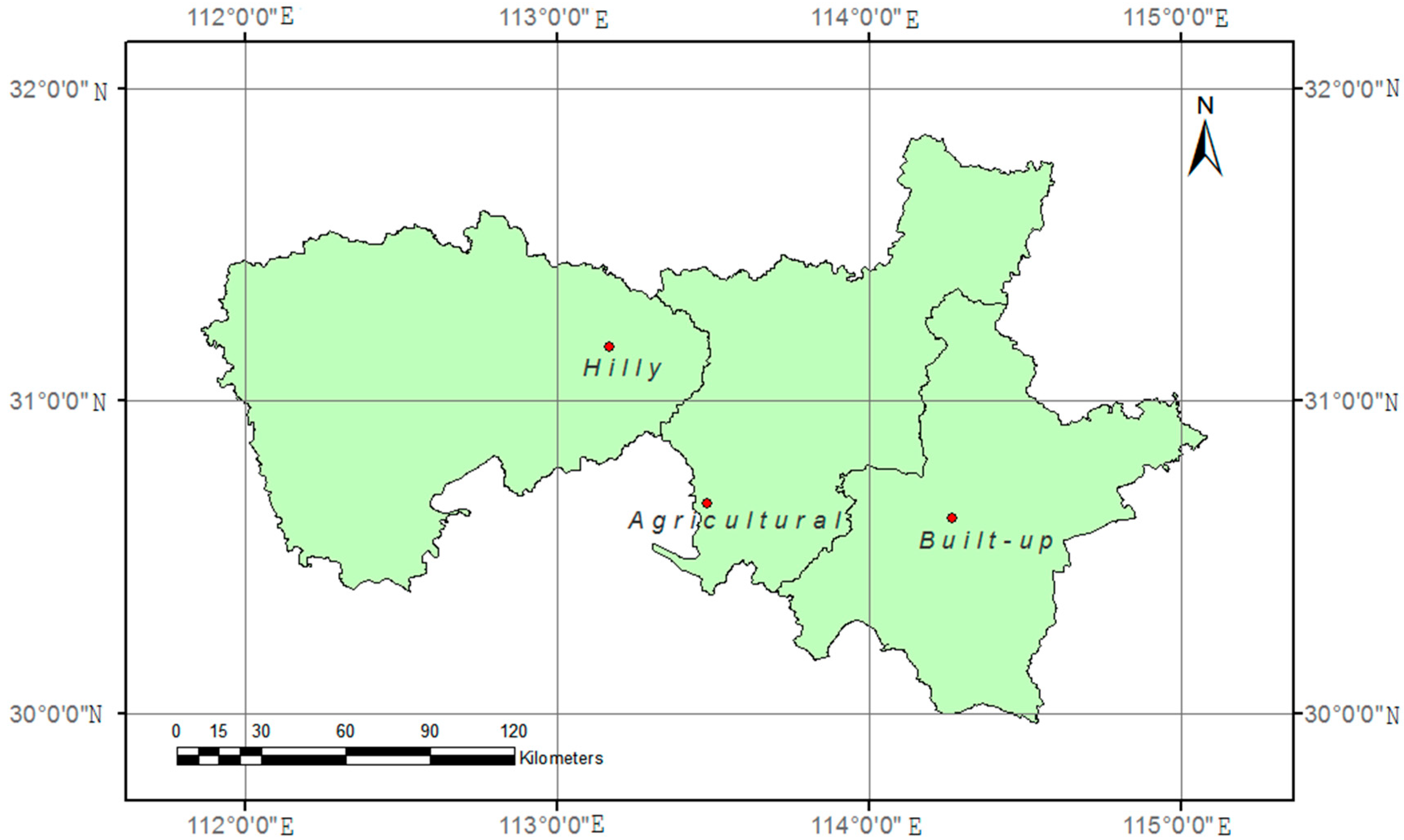
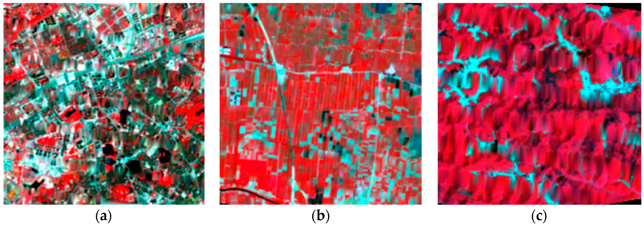
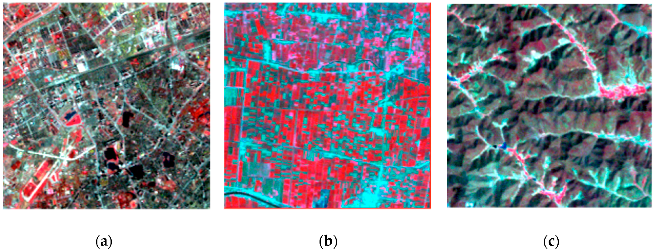
3.1. Experimental Datasets
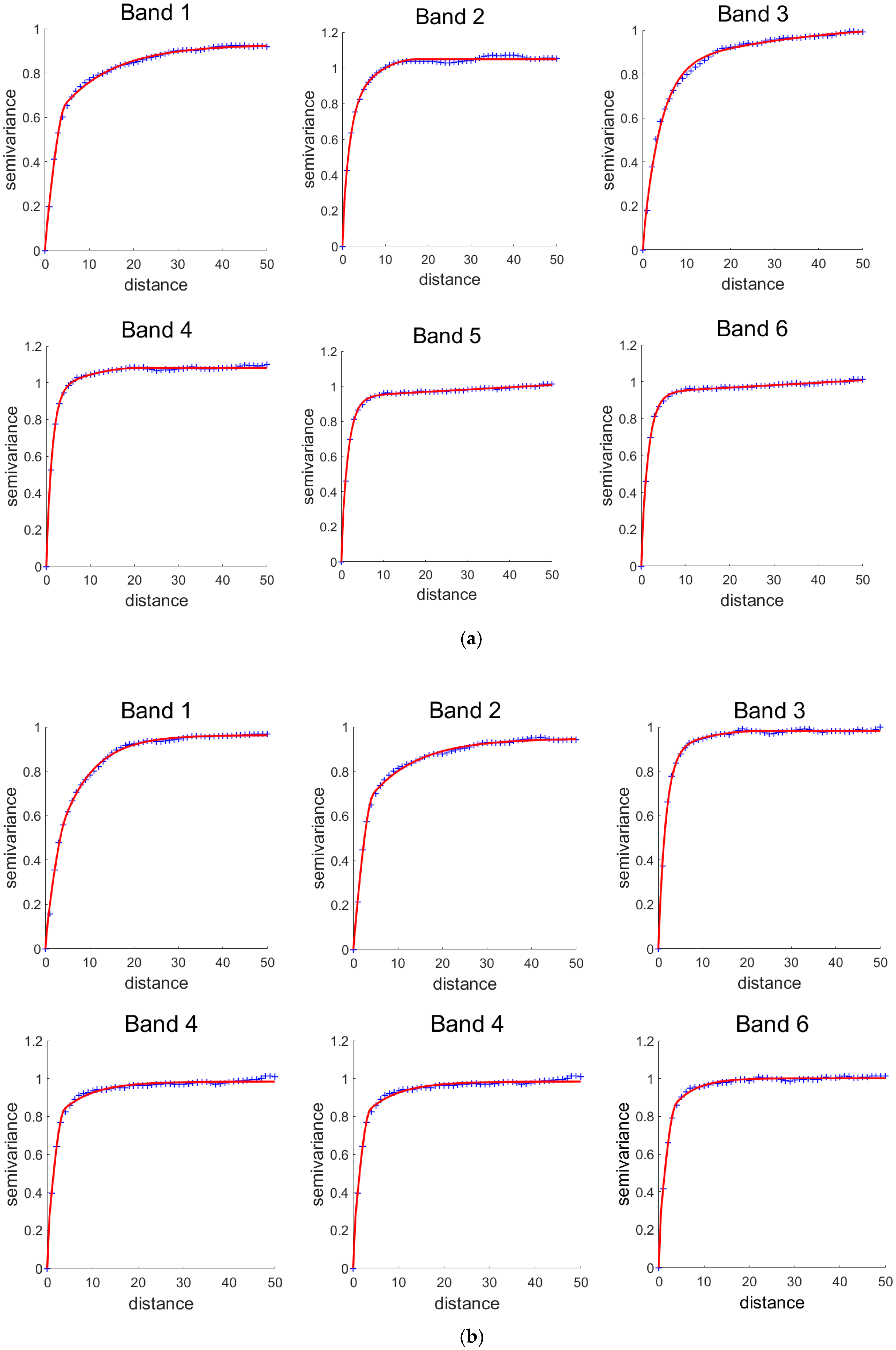
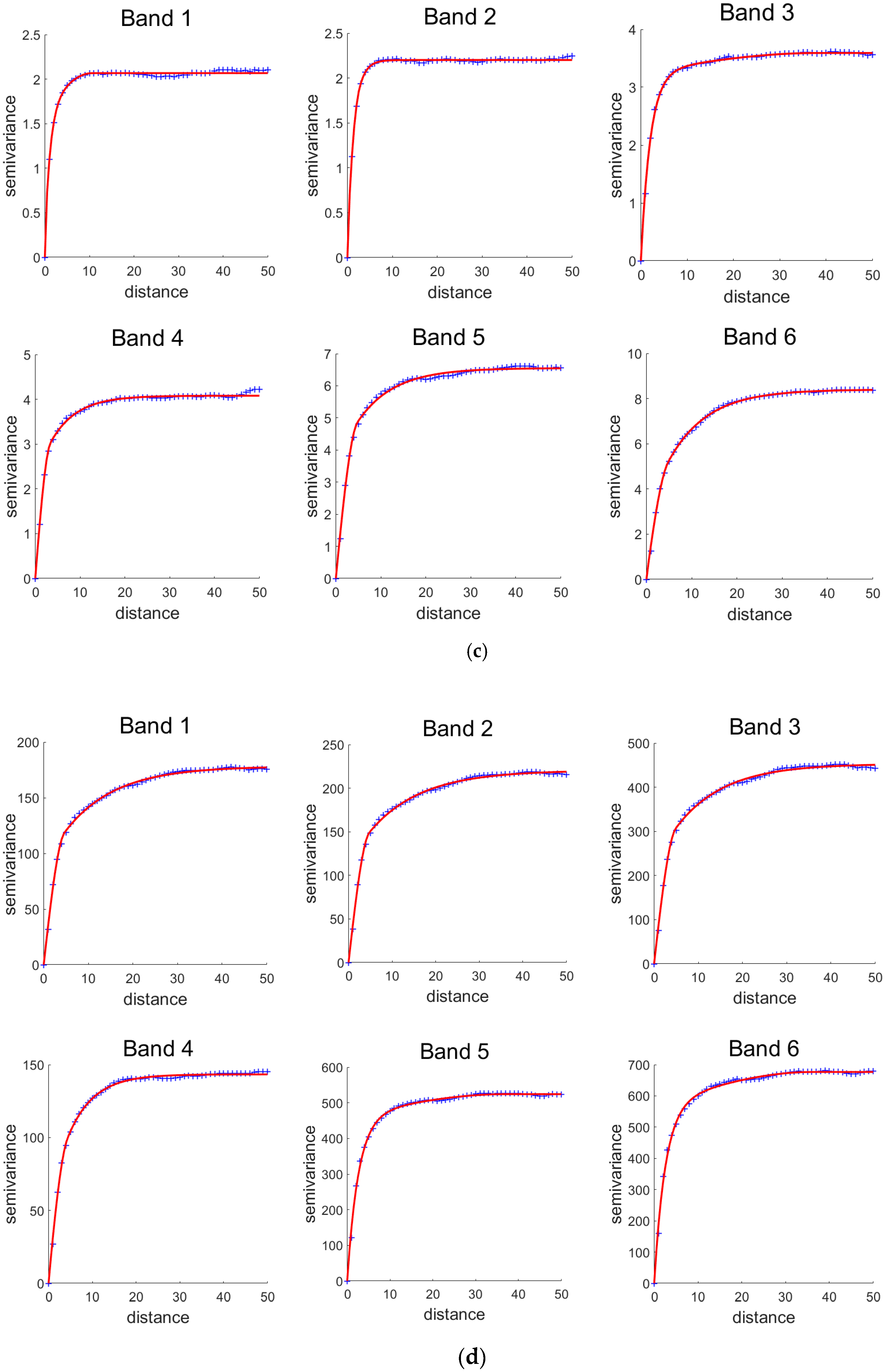
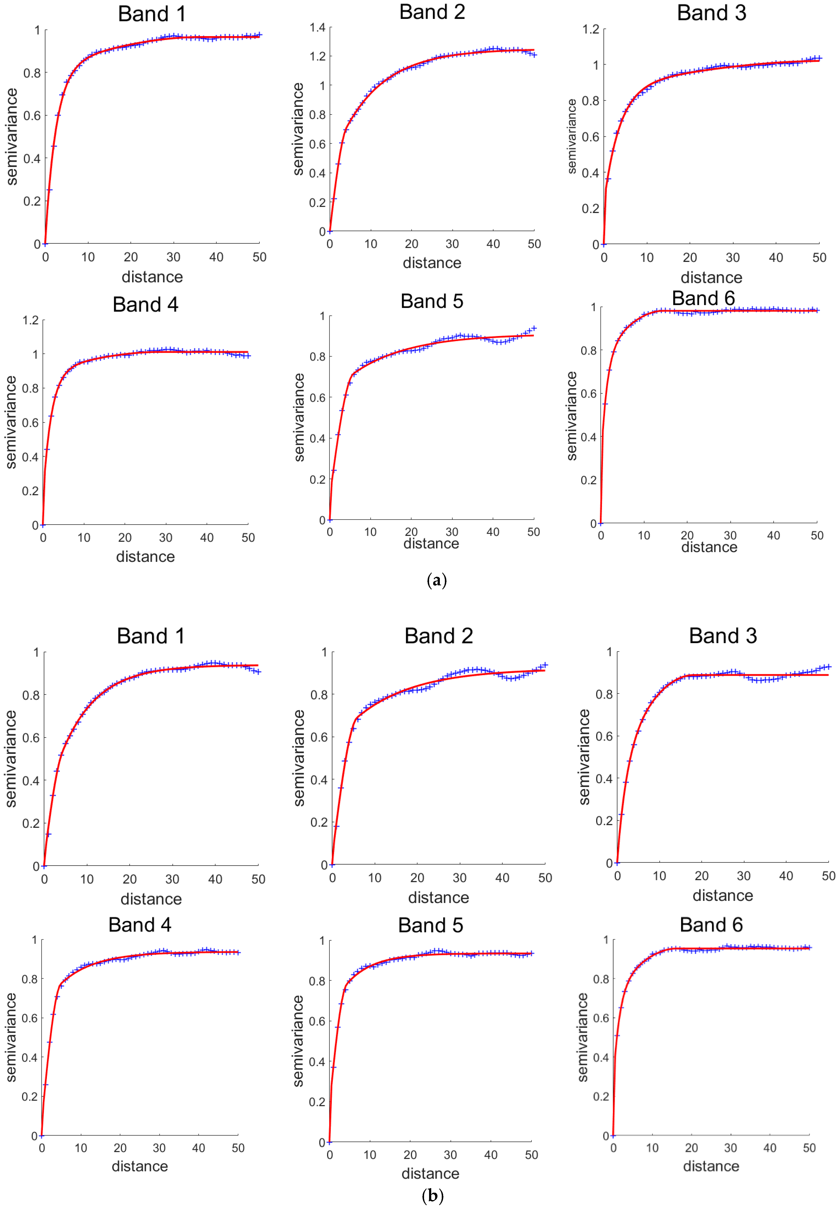
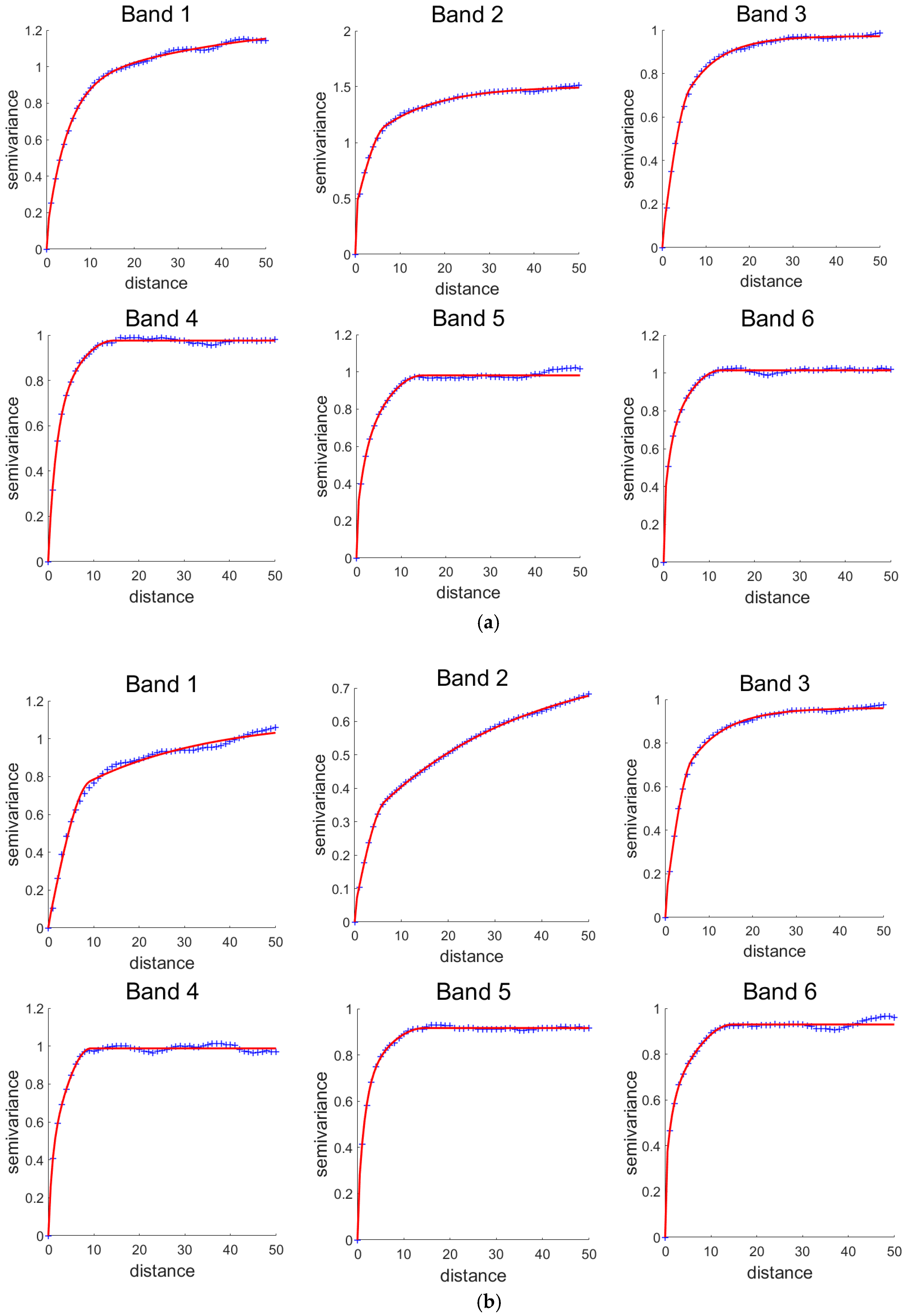
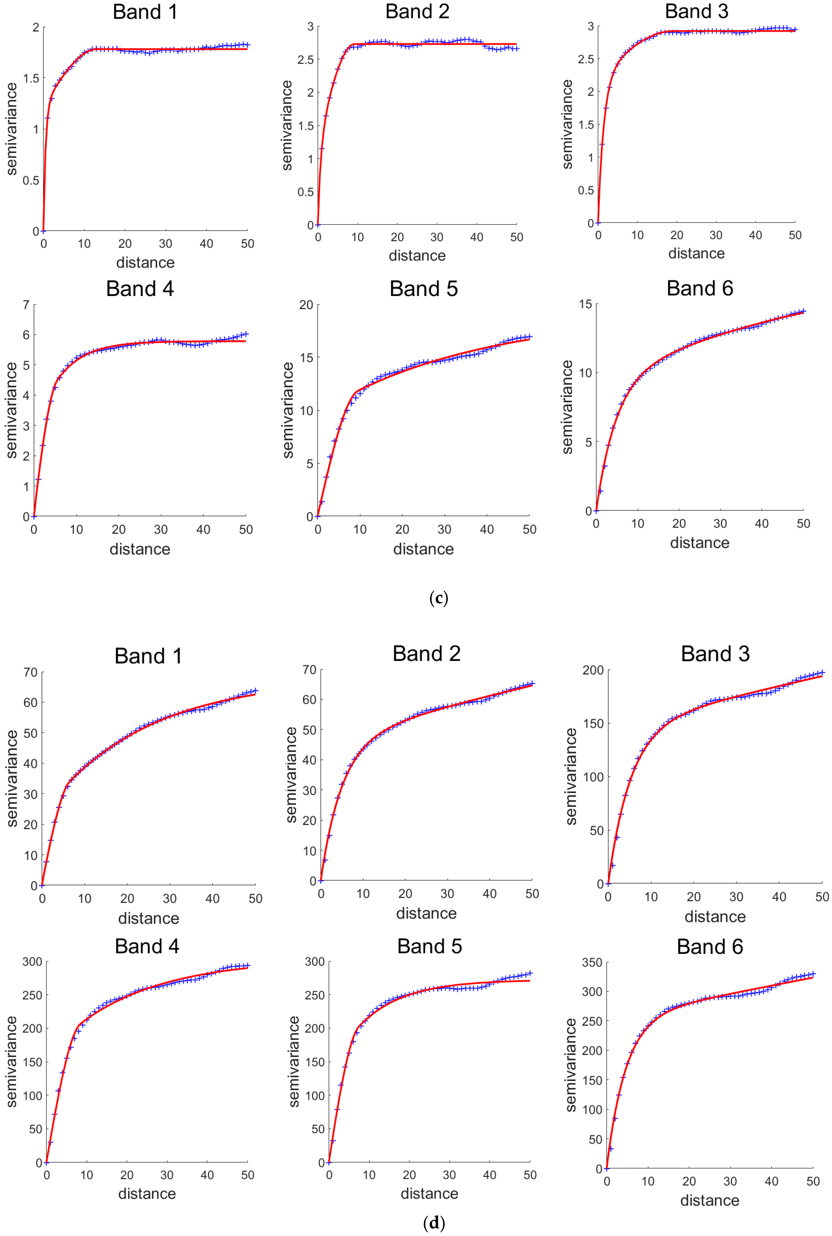
3.2. Experiments with the Landsat ETM+ Dataset
3.3. Experiments with the Landsat TM Dataset and Comparisons Between Landsat ETM+ and TM Datasets
4. Discussion
4.1. Comparing ICA and MNF for Handling Spectral Redundancy
4.2. The Issues of Stationarity Assumptions and Geostatistical Modeling
4.3. Applicabilities of the Proposed Methods and Some Topics for Further Research
5. Conclusions
Author Contributions
Funding
Acknowledgments
Conflicts of Interest
Appendix A


References
- Zhang, J.; Atkinson, P.M.; Goodchild, M.F. Scale in Spatial Information and Analysis; CRC Press: Boca Raton, FL, USA, 2014. [Google Scholar]
- Shannon, C.E. A mathematical theory of communication. Bell Syst. Tech. J. 1948, 27, 379–423. [Google Scholar] [CrossRef]
- Cover, T.M.; Thomas, J.A. Elements of Information Theory, 2nd ed.; John Wiley & Sons Inc.: Hoboken, NJ, USA, 2006. [Google Scholar]
- Goodchild, M.F. The Nature and Value of Geographic Information. In Foundations of Geographic Information Science; Duckham, M., Goodchild, M.F., Worboys, M.F., Eds.; Taylor & Francis: London, UK, 2003; pp. 19–31. [Google Scholar]
- Huck, F.O.; Fales, C.L.; Rahman, Z.-U. An information theory of visual communication. Philos. Trans. R. Soc. A Math. Phys. Eng. Sci. 1996, 354, 2193–2248. [Google Scholar] [CrossRef]
- O’Sullivan, J.A.; Blahut, R.E.; Snyder, D.L. Information-theoretic image formation. IEEE Trans. Inf. Theory. 1998, 44, 2094–2123. [Google Scholar] [CrossRef]
- Peng, H.; Long, F.; Ding, C. Feature selection based on mutual information: Criteria of max-dependency, max-relevance, and min-redundancy. IEEE Trans. Pattern Anal. Mach. Intell. 2005, 27, 1226–1238. [Google Scholar] [CrossRef] [PubMed]
- Meynet, J.; Thiran, J.P. Information theoretic combination of pattern classifiers. Pattern Recognit. 2010, 43, 3412–3421. [Google Scholar] [CrossRef]
- Jia, X.; Kuo, B.C.; Crawford, M.M. Feature mining for hyperspectral image classification. Proc. IEEE. 2013, 101, 676–697. [Google Scholar] [CrossRef]
- Vergara, J.R.; Estévez, P.A. A Review of feature selection methods based on mutual information. Neural Comput. Appl. 2014, 24, 175–186. [Google Scholar] [CrossRef]
- Marinoni, A.; Iannelli, G.C.; Gamba, P. An information theory-based scheme for efficient classification of remote sensing data. IEEE Trans. Geosci. Remote Sens. 2017, 55, 5864–5876. [Google Scholar] [CrossRef]
- Bell, M.R. Information Theory and Radar: Mutual Information and the Design and Analysis of Radar Waveforms and Systems. Ph.D. Thesis, California Institute of Technology, Pasadena, CA, USA, 1988. [Google Scholar] [CrossRef]
- Sheppard, C.J.R.; Larkin, K.G. Information capacity and resolution in three-dimensional imaging. Optik 2003, 113, 548–550. [Google Scholar] [CrossRef][Green Version]
- Weidmann, C.; Vetterli, M. Rate distortion behavior of sparse sources. IEEE Trans. Inf. Theory. 2012, 58, 4969–4992. [Google Scholar] [CrossRef]
- Konings, A.G.; McColl, K.A.; Piles, M.; Entekhabi, D. How many parameters can be maximally estimated from a set of measurements? IEEE Geosci. Remote Sens. Lett. 2015, 12, 1081–1085. [Google Scholar] [CrossRef]
- Zhang, J.; Yang, K.; Liu, F.; Zhang, Y. Information-theoretic characterization and undersampling ratio determination for compressive radar imaging in a simulated environment. Entropy 2015, 17, 5171–5198. [Google Scholar] [CrossRef]
- Chilès, J.P.; Delfiner, P. Geostatistics: Modeling Spatial Uncertainty, 2nd ed.; John Wiley & Sons Inc.: Hoboken, NJ, USA, 2012. [Google Scholar]
- Chen, T.M.; Staelin, D.H.; Arps, R.B. Information content analysis of landsat image data for compression. IEEE Trans. Geosci. Remote Sens. 1987, 25, 499–501. [Google Scholar] [CrossRef]
- Aiazzi, B.; Baronti, S.; Alparone, L. Lossless compression of hyperspectral images using multiband lookup tables. IEEE Signal Process. Lett. 2009, 16, 481–484. [Google Scholar] [CrossRef]
- Frost, V.S.; Shanmugan, K.S. The information content of synthetic aperture radar images of terrain. IEEE Trans. Aerosp. Electron. Syst. 1983, 5, 768–774. [Google Scholar] [CrossRef]
- Blacknell, D.; Oliver, C.J. Information content of coherent images. J. Phys. D Appl. Phys. 1993, 26, 1364–1370. [Google Scholar] [CrossRef]
- Price, J.C. Comparison of the information-content of data from the landsat-4 thematic mapper and the multispectral scanner. IEEE Trans. Geosci. Remote Sens. 1984, 3, 272–281. [Google Scholar] [CrossRef]
- Horler, D.N.H.; Ahern, F.J. Forestry information content of thematic mapper data. Int. J. Remote Sens. 1985, 7, 405–428. [Google Scholar] [CrossRef]
- Nielsen, A.A.; Larsen, R. Restoration of geris data using the maximum noise fractions transform. In Proceedings of the International Airborne Remote Sensing Conference and Exhibition, Strasbourg, France, 11–15 September 1994; pp. 557–568. [Google Scholar]
- Green, A.A.; Berman, M.; Switzer, P.; Craig, M.D. A Transformation for ordering multispectral data in terms of image quality with implications for noise removal. IEEE Trans. Geosci. Remote Sens. 1988, 26, 65–74. [Google Scholar] [CrossRef]
- Razlighi, Q.R.; Kehtarnavaz, N.; Nosratinia, A. Computation of image spatial entropy using quadrilateral markov random field. IEEE Trans. Image Process. 2009, 18, 2629–2639. [Google Scholar] [CrossRef]
- Wang, J.; Zhang, K.; Tang, S. Spectral and spatial decorrelation of landsat-TM data for lossless compression. IEEE Trans. Geosci. Remote Sens. 1995, 33, 1277–1285. [Google Scholar] [CrossRef]
- Aiazzi, B.; Alparone, L.; Barducci, A.; Baronti, S.; Pippi, I. Estimating noise and information of multispectral imagery. Opt. Eng. 2002, 41, 656–668. [Google Scholar] [CrossRef]
- Hyvärinen, A. Fast and robust fixed-point algorithms for independent component analysis. IEEE Trans. Neural Netw. 1999, 10, 626–634. [Google Scholar] [CrossRef] [PubMed]
- Falco, N.; Benediktsson, J.A.; Bruzzone, L. A Study on the effectiveness of different independent component analysis algorithms for hyperspectral image classification. IEEE J. Sel. Top. Appl. Earth Observ. 2014, 7, 2183–2199. [Google Scholar] [CrossRef]
- Boluwade, A.; Madramootoo, C.A. Geostatistical independent simulation of spatially correlated soil Variables. Comput. Geosci. 2015, 85, 3–15. [Google Scholar] [CrossRef]
- Li, Z.; Huang, P. Quantitative measures for spatial information of maps. Int. J. Geogr. Inf. Sci. 2002, 16, 699–709. [Google Scholar] [CrossRef]
- Harrie, L.; Stigmar, H. An evaluation of measures for quantifying map information. ISPRS J. Photogramm. Remote Sens. 2010, 65, 266–274. [Google Scholar] [CrossRef]
- Myers, D.E. To be or not to be… stationary? That is the question. Math. Geol. 1989, 21, 347–362. [Google Scholar] [CrossRef]
- Chou, Y.M.; Polansky, A.M.; Mason, R.L. Transforming nonnormal data to normality in statistical process-control. J. Qual. Technol. 1998, 30, 133–141. [Google Scholar] [CrossRef]
- Gong, W.; Yang, D.; Gupta, H.V.; Nearing, G. Estimating information entropy for hydrological data: One-dimensional case. Water Resour. Res. 2014, 50, 5003–5018. [Google Scholar] [CrossRef]
- Cressie, N. Fitting Variogram models by weighted least-squares. J. Int. Assoc. Math. Geol. 1985, 17, 563–586. [Google Scholar] [CrossRef]
- Woodcock, C.E.; Strahler, A.H.; Jupp, D.L.B. The use of variograms in remote sensing: I. Scene models and simulated images. Remote Sens. Environ. 1988, 25, 323–348. [Google Scholar] [CrossRef]
- Woodcock, C.E.; Strahler, A.H.; Jupp, D.L.B. The use of variograms in remote sensing: II. Real digital images. Remote Sens. Environ. 1988, 25, 349–379. [Google Scholar] [CrossRef]
- Asmat, A.; Atkinson, P.M.; Foody, G.M. Geostatistically estimated image noise is a function of variance in the underlying signal. Int. J. Remote Sens. 2010, 31, 1009–1025. [Google Scholar] [CrossRef]
- Phiri, D.; Morgenroth, J. Developments in landsat land cover classification methods: A review. Remote Sens. 2017, 9, 967. [Google Scholar] [CrossRef]
- Nunes, M.A.; Taylor, S.L.; Eckley, I.A. A Multiscale test of spatial stationarity for textured images in R. R J. 2014, 6, 20–30. [Google Scholar] [CrossRef]
- Journel, A.; Zhang, T. The necessity of a multiple-point prior model. Math. Geol. 2006, 38, 591–610. [Google Scholar] [CrossRef]
- Tan, X.; Tahmasebi, P.; Caers, J. Comparing training-image based algorithms using an analysis of distance. Math. Geosci. 2014, 46, 149–169. [Google Scholar] [CrossRef]
- Feng, J.; Jiao, L.; Liu, F.; Sun, T.; Zhang, X. Mutual-information-based semi-supervised hyperspectral band selection with high discrimination, high information, and low redundancy. IEEE Trans. Geosci. Remote Sens. 2015, 53, 2956–2969. [Google Scholar] [CrossRef]
- Larsen, R.; Hilger, K.B. Statistical shape analysis using non-euclidean metrics. Med. Image Anal. 2003, 7, 417–423. [Google Scholar] [CrossRef]


| Image Subsets | ICA- and Normal- Transformed Image Z″ Bands | Transform Type | Parameters | ||||
|---|---|---|---|---|---|---|---|
| Built-Up | 1 | Su | 3.50 | 1.92 | − 0.73 | 0.51 | 0.13 |
| 2 | Su | 1.77 | 2.25 | − 1.97 | 1.53 | 0.09 | |
| 3 | Su | 0.60 | 1.10 | − 1.32 | 0.54 | 0.17 | |
| 4 | Su | − 0.20 | 1.69 | − 5.14 | 1.36 | 0.24 | |
| 5 | Su | 0.06 | 1.40 | − 0.94 | 1.03 | 0.05 | |
| 6 | Su | − 0.42 | 1.45 | 12.70 | 0.97 | 0.10 | |
| Agricultural | 1 | Su | 0.73 | 1.04 | 0.59 | 0.50 | 0.09 |
| 2 | Su | − 0.02 | 1.15 | 0.11 | 0.52 | 0.34 | |
| 3 | Su | − 0.71 | 1.15 | 0.11 | 0.52 | 0.49 | |
| 4 | Su | − 0.49 | 1.12 | − 0.40 | 0.56 | 0.19 | |
| 5 | Su | 0.03 | 2.01 | 0.04 | 1.72 | 0.05 | |
| 6 | Su | 0.24 | 1.93 | 0.23 | 1.60 | 0.06 | |
| Hilly | 1 | Su | − 0.42 | 0.50 | − 0.45 | 0.08 | 0.03 |
| 2 | Su | − 0.30 | 2.71 | − 0.15 | 0.55 | 1.53 | |
| 3 | Su | − 0.56 | 2.77 | 0.54 | 2.45 | 0.05 | |
| 4 | Su | − 0.16 | 1.22 | − 0.09 | 0.72 | 0.19 | |
| 5 | Su | − 0.50 | 2.88 | − 0.42 | 2.40 | 0.14 | |
| 6 | Su | − 0.06 | 0.91 | − 0.05 | 0.43 | 0.11 | |
| Bands | Built-Up | Agricultural | Hilly | ||||||||||||
|---|---|---|---|---|---|---|---|---|---|---|---|---|---|---|---|
| Nug | Exp | Sph | Nug | Exp | Sph | Nug | Exp | Sph | |||||||
| Sill | Range | Sill | Range | Sill | Range | Sill | Range | Sill | Range | Sill | Range | ||||
| 1 | 0.02 | 0.40 | 35.61 | 0.51 | 4.78 | 0.01 | 0.83 | 7.70 | 0.13 | 36.18 | 0.08 | 0.85 | 14.44 | 0.25 | 68.14 |
| 2 | 0.08 | 0.76 | 5.41 | 0.20 | 17.31 | 0.01 | 0.80 | 31.21 | 0.45 | 4.13 | 0.40 | 0.60 | 38.46 | 0.51 | 6.61 |
| 3 | 0.02 | 0.83 | 12.05 | 0.15 | 63.15 | 0.22 | 0.66 | 11.02 | 0.14 | 52.08 | 0.04 | 0.55 | 22.94 | 0.38 | 6.35 |
| 4 | 0.01 | 0.96 | 4.05 | 0.11 | 20.56 | 0.15 | 0.76 | 6.14 | 0.11 | 28.52 | 0.01 | 0.69 | 5.62 | 0.27 | 14.37 |
| 5 | 0.06 | 0.88 | 4.91 | 0.17 | 191.30 | 0.11 | 0.30 | 41.18 | 0.50 | 5.84 | 0.19 | 0.45 | 6.24 | 0.34 | 14.67 |
| 6 | 0.10 | 0.42 | 23.75 | 0.49 | 4.72 | 0.25 | 0.55 | 4.24 | 0.18 | 14.40 | 0.27 | 0.44 | 4.87 | 0.30 | 12.52 |
| Bands | Built-Up | Agricultural | Hilly | ||||||||||||
|---|---|---|---|---|---|---|---|---|---|---|---|---|---|---|---|
| Nug | Exp | Sph | Nug | Exp | Sph | Nug | Exp | Sph | |||||||
| Sill | Range | Sill | Range | Sill | Range | Sill | Range | Sill | Range | Sill | Range | ||||
| 1 | 0.04 | 0.69 | 21.62 | 0.23 | 4.74 | 0.02 | 0.68 | 24.80 | 0.24 | 4.34 | 0.01 | 0.46 | 83.57 | 0.63 | 9.24 |
| 2 | 0.01 | 0.38 | 31.86 | 0.56 | 4.60 | 0.03 | 0.35 | 40.94 | 0.53 | 5.92 | 0.04 | 0.52 | 98.35 | 0.23 | 6.42 |
| 3 | 0.01 | 0.90 | 5.12 | 0.08 | 22.71 | 0.01 | 0.58 | 7.69 | 0.30 | 17.93 | 0.07 | 0.49 | 25.26 | 0.40 | 6.16 |
| 4 | 0.14 | 0.25 | 20.66 | 0.59 | 3.83 | 0.06 | 0.29 | 26.17 | 0.59 | 4.95 | 0.02 | 0.44 | 2.55 | 0.53 | 9.29 |
| 5 | 0.13 | 0.82 | 7.06 | 0.07 | 0.28 | 0.18 | 0.29 | 19.80 | 0.47 | 4.34 | 0.11 | 0.60 | 4.75 | 0.20 | 14.46 |
| 6 | 0.04 | 0.82 | 5.18 | 0.12 | 18.85 | 0.27 | 0.50 | 5.02 | 0.18 | 16.22 | 0.25 | 0.36 | 4.34 | 0.32 | 14.65 |
| Bands | Built-Up | Agricultural | Hilly | ||||||||||||
|---|---|---|---|---|---|---|---|---|---|---|---|---|---|---|---|
| Nug | Exp | Sph | Nug | Exp | Sph | Nug | Exp | Sph | |||||||
| Sill | Range | Sill | Range | Sill | Range | Sill | Range | Sill | Range | Sill | Range | ||||
| 1 | 0.16 | 90.36 | 33.46 | 87.68 | 4.70 | 0.37 | 3.65 | 23.80 | 28.42 | 6.32 | 0.31 | 44.64 | 72.13 | 23.15 | 6.60 |
| 2 | 0.22 | 106.70 | 35.34 | 113.48 | 4.81 | 0.26 | 35.54 | 29.33 | 46.23 | 6.00 | 0.13 | 45.77 | 15.01 | 30.43 | 114.56 |
| 3 | 0.21 | 229.84 | 32.43 | 222.89 | 4.94 | 0.17 | 93.51 | 29.57 | 130.54 | 6.00 | 0.31 | 145.76 | 15.72 | 111.37 | 170.07 |
| 4 | 0.36 | 92.32 | 17.45 | 50.66 | 4.37 | 0.45 | 98.77 | 37.34 | 55.39 | 6.29 | 0.23 | 143.89 | 63.52 | 158.89 | 8.54 |
| 5 | 0.21 | 463.29 | 7.85 | 60.80 | 36.81 | 0.10 | 207.50 | 18.55 | 105.67 | 5.01 | 0.11 | 136.79 | 33.07 | 135.10 | 7.50 |
| 6 | 0.16 | 574.04 | 7.65 | 12.34 | 36.02 | 0.44 | 218.71 | 19.61 | 151.30 | 5.57 | 0.30 | 142.89 | 87.95 | 204.42 | 8.94 |
| Image Subsets | Built-Up | Agricultural | Hilly |
|---|---|---|---|
| Joint entropy h() | 9.88 | 9.73 | 9.84 |
| 0.78 | 1.22 | 1.94 | |
| Joint entropy h() | 9.10 | 8.51 | 7.90 |
| Difference between h(Z) and h() | 14.68 | 13.79 | 14.11 |
| Joint entropy h(Z) | 23.78 | 22.30 | 22.01 |
| Noise joint entropy h(N) | 5.56 | 6.51 | 5.57 |
| Mutual information | 18.22 | 15.79 | 16.44 |
| Methods | Experimental Image Subsets | ||
|---|---|---|---|
| Built-Up | Agricultural | Hilly | |
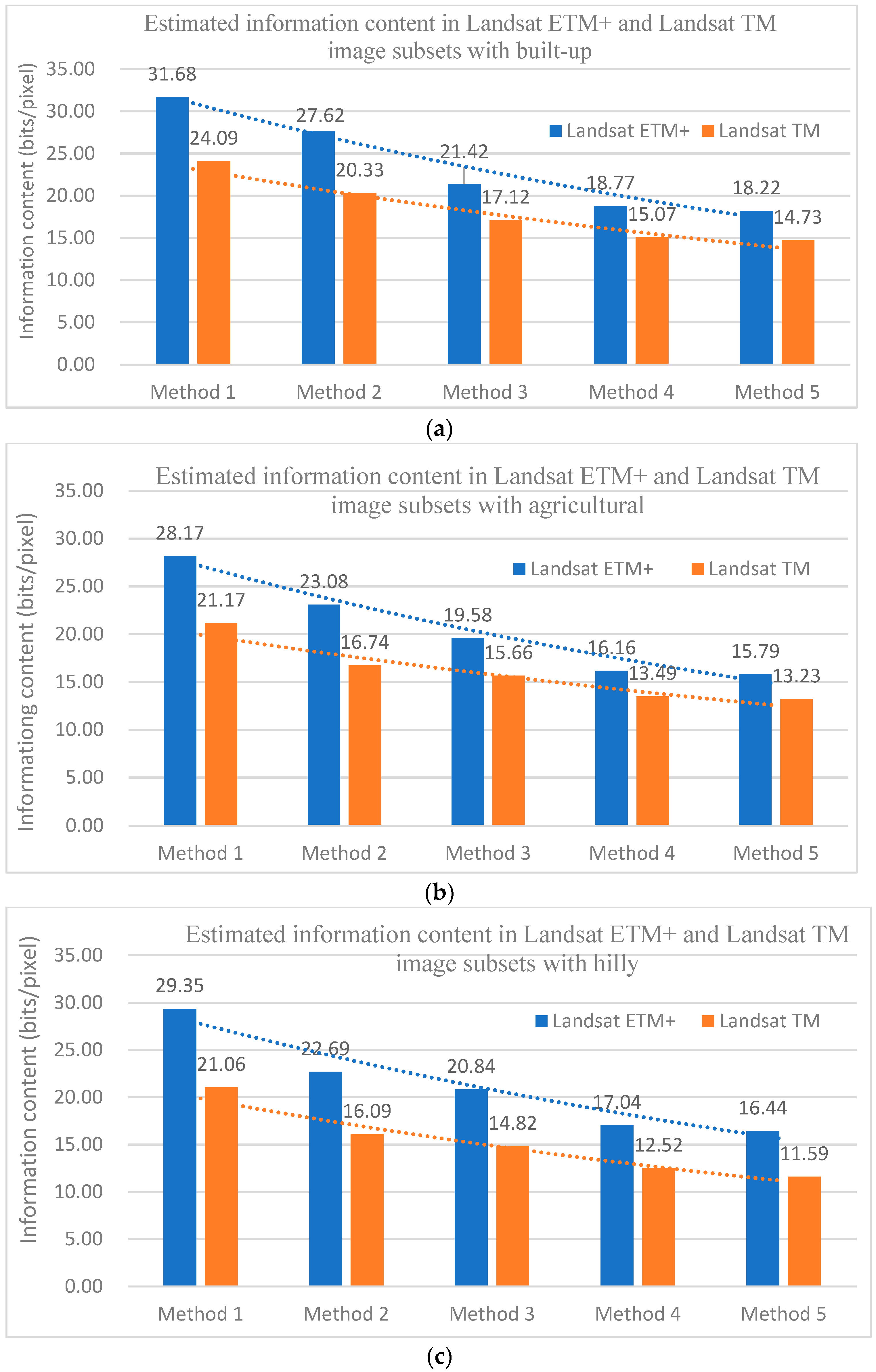
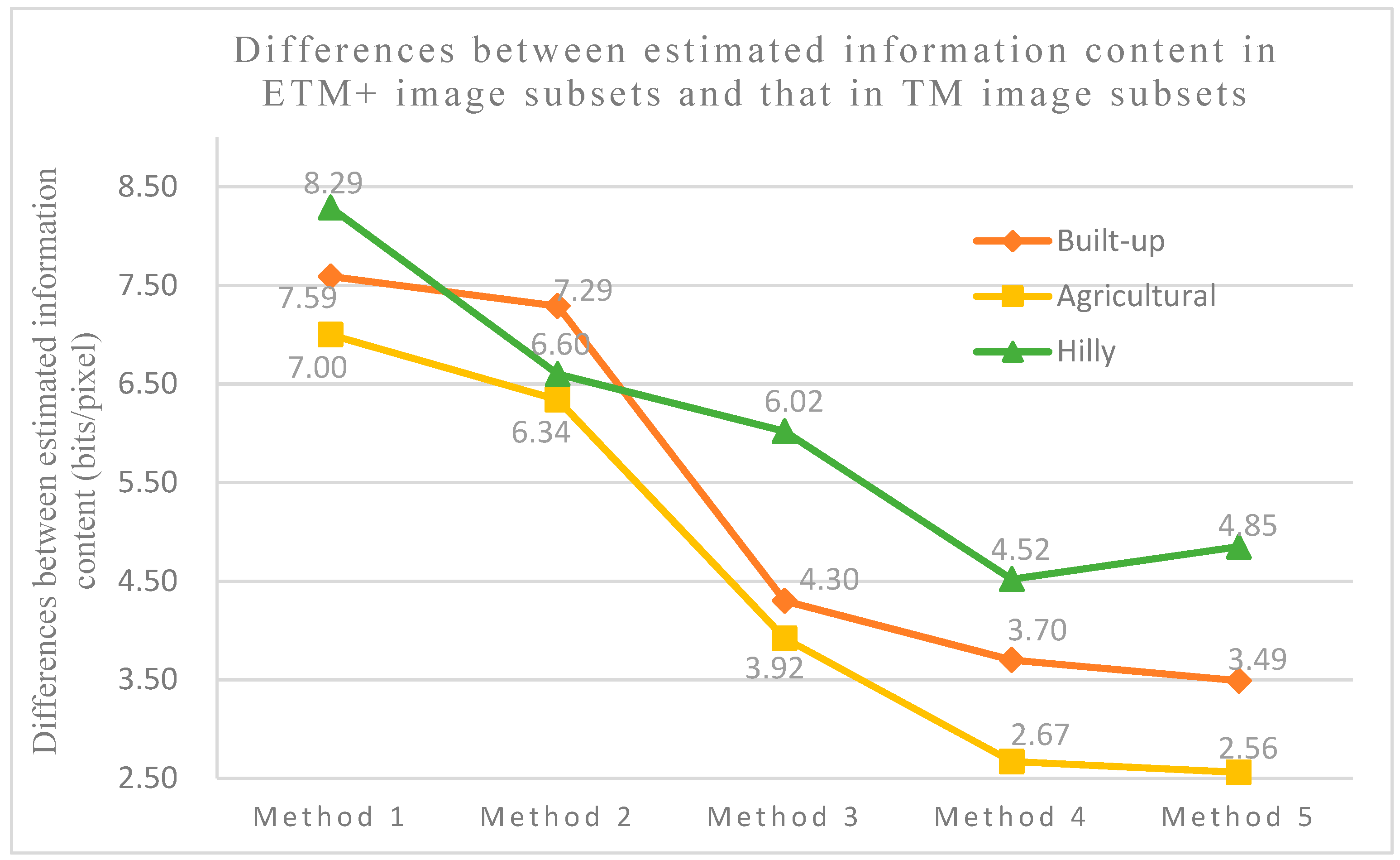
| 1. Not considering spectral and spatial dependences and non-normality | 31.68 | 28.17 | 29.35 |
| 2. Considering spatial dependence only | 27.62 | 23.08 | 22.69 |
| 3. Considering spectral dependence (via ICA) only | 21.42 | 19.58 | 20.84 |
| 4. Considering spectral (via ICA) and spatial dependences | 18.77 | 16.16 | 17.04 |
| 5. Considering spectral (via ICA) and spatial dependences and non-normality | 18.22 | 15.79 | 16.44 |
| Methods | Experimental Image Subsets | ||
|---|---|---|---|
| Built-Up | Agricultural | Hilly | |
| 1. Not considering spectral dependence, spatial dependences, and non-normality | 24.09 | 21.17 | 21.06 |
| 2. Considering spatial dependence only | 20.33 | 16.74 | 16.09 |
| 3. Considering spectral dependence (via ICA) only | 17.12 | 15.66 | 14.82 |
| 4. Considering spectral (via ICA) and spatial dependences | 15.07 | 13.49 | 12.52 |
| 5. Considering spectral (via ICA) and spatial dependences and non-normality | 14.73 | 13.23 | 11.59 |
| Methods | Data | Experimental Image Subsets | ||
|---|---|---|---|---|
| Built-Up | Agricultural | Hilly | ||
| 6. Considering spectral dependence (via MNF) only | ETM+ | 23.21 | 21.33 | 22.30 |
| TM | 19.90 | 16.50 | 16.92 | |
| 7. Considering spectral (via MNF) and spatial dependences | ETM+ | 20.39 | 17.72 | 18.30 |
| TM | 17.96 | 14.27 | 14.23 | |
© 2020 by the authors. Licensee MDPI, Basel, Switzerland. This article is an open access article distributed under the terms and conditions of the Creative Commons Attribution (CC BY) license (http://creativecommons.org/licenses/by/4.0/).
Share and Cite
Zhang, Y.; Zhang, J.; Yang, W. Quantifying Information Content in Multispectral Remote-Sensing Images Based on Image Transforms and Geostatistical Modelling. Remote Sens. 2020, 12, 880. https://doi.org/10.3390/rs12050880
Zhang Y, Zhang J, Yang W. Quantifying Information Content in Multispectral Remote-Sensing Images Based on Image Transforms and Geostatistical Modelling. Remote Sensing. 2020; 12(5):880. https://doi.org/10.3390/rs12050880
Chicago/Turabian StyleZhang, Ying, Jingxiong Zhang, and Wenjing Yang. 2020. "Quantifying Information Content in Multispectral Remote-Sensing Images Based on Image Transforms and Geostatistical Modelling" Remote Sensing 12, no. 5: 880. https://doi.org/10.3390/rs12050880
APA StyleZhang, Y., Zhang, J., & Yang, W. (2020). Quantifying Information Content in Multispectral Remote-Sensing Images Based on Image Transforms and Geostatistical Modelling. Remote Sensing, 12(5), 880. https://doi.org/10.3390/rs12050880