Advanced Machine Learning Optimized by The Genetic Algorithm in Ionospheric Models Using Long-Term Multi-Instrument Observations

Abstract

The ionospheric delay is of paramount importance to radio communication, satellite navigation and positioning. It is necessary to predict high-accuracy ionospheric peak parameters for single frequency receivers. In this study, the state-of-the-art artificial neural network (ANN) technique optimized by the genetic algorithm is used to develop global ionospheric models for predicting foF2 and hmF2. The models are based on long-term multiple measurements including ionospheric peak frequency model (GIPFM) and global ionospheric peak height model (GIPHM). Predictions of the GIPFM and GIPHM are compared with the International Reference Ionosphere (IRI) model in 2009 and 2013 respectively. This comparison shows that the root-mean-square errors (RMSEs) of GIPFM are 0.82 MHz and 0.71 MHz in 2013 and 2009, respectively. This result is about 20%–35% lower than that of IRI. Additionally, the corresponding hmF2 median errors of GIPHM are 20% to 30% smaller than that of IRI. Furthermore, the ANN models present a good capability to capture the global or regional ionospheric spatial-temporal characteristics, e.g., the equatorial ionization anomaly and Weddell Sea anomaly. The study shows that the ANN-based model has a better agreement to reference value than the IRI model, not only along the Greenwich meridian, but also on a global scale. The approach proposed in this study has the potential to be a new three-dimensional electron density model combined with the inclusion of the upcoming Constellation Observing System for Meteorology, Ionosphere and Climate (COSMIC-2) data.

1. Introduction

The F2 layer (roughly 150–500 km above the ground) is the most important ionospheric layer, especially during the solar-terrestrial quiet time. This layer is populated by huge numbers of ions and electrons under the dynamic equilibrium condition [1]. The critical frequency of F2 layer (foF2) and its corresponding peak height (hmF2) are the common parameters to represent ionospheric variations. These two parameters play a significant role in the long-distance high-frequency (HF) radio communications since the critical frequency determines the maximum usable frequency according to the electromagnetic theory [2]. The importance of foF2 in the HF radio communication field has driven the development of many ionospheric and HF radio propagation models. With the advancements of space-borne and ground-based instruments and data processed techniques, more attention has been paid to the development and improvement of these ionospheric models [3].

In the previous studies, the artificial neural network (ANN), nonlinear least squares and AdaBoost techniques have been used to predict ionospheric variations with a satisfactory accuracy [4,5,6,7]. Among them, the ANN technique has proven to be a successful tool in the modeling of ionospheric variations as well as solving the forecast problems in many geophysical applications over a single station, regional area and global scale [3,8,9,10]. The neural network was first applied to build the foF2 model over the Grahamstown station (33°S, 26°E) using the data range set of 1973–1983 [11]. This model can predict the daily noon foF2 value with a root-mean-square error (RMSE) of 0.95 MHz and the monthly averaged RMSE value was 0.48 MHz. Afterward, this approach has been widely applied in the Asia/Pacific sector [5], equatorial region [12], European region [13] and the auroral zone [14]. These studies showed an improvement in the accuracy of the ANN-based models over the International Reference Ionosphere (IRI) model.

With the advancement of data acquisition, more ionospheric measurements have become available for the global modelling of foF2. For instance, Oyeyemi et al. [15] used the foF2 data from 59 globally distributed ionospheric stations to establish the ANN-based prediction model NN2; the RMSE values of NN2 is better than the International Radio Consultative Committee (CCIR) model by an order of 15–16%. In the past few decades, the Global Navigation Satellite System (GNSS) radio occultation technique showed its potential to be a powerful tool in probing the ionospheric electron density over the globe [16]. Until now, the CHAMP (Challenging Minisatellite Payload), GRACE (Gravity Recovery and Climate Experiment) and COSMIC (Constellation Observing System for Meteorology, Ionosphere and Climate) satellite missions have collected millions of ionospheric profiles, which include the three-dimensional structure of electron density with unprecedented detail [6].

The combination of space-borne and ground-based ionospheric measurements opens a new way to ionospheric modelling with higher accuracy. A good example is the ANN-Based Ionospheric Model (ANNIM) developed by Tulasi Ram et al. [17]. This model was fed by multiple data from CHAMP, GRACE, COSMIC and global ground-based digisonde stations, which are first binned into 840 spatial grids with a spatial resolution of 5° in dip latitude and 15° in geographic longitude. A neural network is then trained at each grid using the error back-propagation algorithm. Their results presented the outperformance of ANNIM in the IRI model: the RMSE values of peak electron density (NmF2) in solar maximum year 2002 and solar minimum year 2009 are 3.4 × 10⁵ electrons/cm³ and 1.5 × 10⁵ electrons/cm³, respectively, and the corresponding RMSE values of hmF2 in 2002 and 2009 are 29 km and 25 km, respectively. The accuracy of ANNIM has a great increasing potential, which is related to the discrepancy between the measurements obtained from different observational carriers.

Many previous studies have revealed a discrepancy of the peak parameters between the COSMIC and ionosonde observations over the European region [18], Australia [19], Brazilian region [20] and China [21]. The discrepancy is dependent on local time, latitude and solar activity, especially in the equator and polar region, the correlation coefficient between COSMIC measurement and ionosonde observations is smaller than 0.8 sometimes. Therefore, the discrepancy between different source data should be corrected before establishing the ionospheric model for higher accuracy.

This paper is structured as follows. The discrepancy between COSMIC data and ionosonde measurements was first corrected, and the quality of electron density profiles and ionosonde observational points were evaluated for quality control. Then the data after the quality control were trained to develop a global ANN-based ionospheric model predicting foF2 and hmF2. To avoid the “local minimum” effect in the traditional neural network applications, the initial weights of the artificial neural network were optimized by the genetic algorithm. In addition, the new ANN model developed in this paper was validated with reference values and the IRI model to evaluate the models’ performance and its capability/capacity in capturing global ionospheric spatial-temporal characteristics.

2. Materials and Methods

2.1. Materials

In the study, the global distributed ionospheric electron density profiles obtained from the FORMOSAT-3/COSMIC mission and the observations derived from global ionosonde stations during 2007–2016 were used to build the ionospheric models for predicting foF2 and hmF2. The COSMIC profiles were provided by the University Corporation for Atmospheric Research (UCAR) community programs (https://www.cosmic.ucar.edu/), and the ionosonde measurements were supplied from the Digisonde Global Ionosphere Radio Observatory (GIRO) (http://giro.uml.edu/didbase/scaled.php), as shown in Figure 1. Figure 1a shows the daily variation of 10.7 cm solar flux (F10.7) during 2007–2016; the solar activity during 2007–2010 was relatively low, and the intensity increased from 2011 to 2014 with the maximum value of 250SFU. Figure 1b shows the number of COSMIC profiles each month selected in the study; during 2007–2010, the COSMIC constellation provided about 2000 uniformly distributed electron density profiles per day globally. Because of the operational failure of some microsatellites, the number of GNSS radio occultations gradually decreased from 2011 to 2016 (http://cdaac-www.cosmic.ucar.edu/cdaac/index.html). Figure 1c shows the number of ionosonde observations each month obtained from GIRO network in the same time range, and the 108 stations used in the work distribute in the subfigure of Figure 1c. With the increase of the Digisonde in the global, the Digisonde observations were increasing steadily from 2007 to 2016. It is noted that the COSMIC occultation only measured peak density directly, rather than peak frequency, the two parameters can be transformed as follows [22]:

$$NmF2=1.24\times {10}^{10}\times {(foF2)}^2$$

(1)

In the initial stage of data processing, all the observational data should be checked for quality control. For COSMIC profiles, the measured profiles were simulated by Chapman-α function [23], and the correlation coefficients between measured profiles and simulated profiles were computed. The measured profiles with a correlation coefficient of less than 0.85 were removed in the quality control process. For ionosonde data, the observations that exceeded the bounds determined by mean ± 1.5 times the standard deviation were eliminated [24]. After the process of quality control, the rate of qualified samples was about 85%. In addition, the parameters that represented the solar-terrestrial environment were also used as the input data of neural network; here, the parameters F10.7, sunspot number (SSN), solar wind speed (Vsw), Dst, Kp and Ap were provided by the Space Physics Data Facility of National Aeronautics and Space Administration (NASA) (https://omniweb.gsfc.nasa.gov/).

Previous studies have reported that there were great nonlinear discrepancies between COSMIC’s data and ionosonde’s observations [25,26,27]; here, we proposed a method to reduce the remarkable discrepancies. The global ionospheric data during 2007–2016 (same as in Figure 1) observed by COSMIC/ionosonde was utilized to develop the ionospheric models for foF2 and hmF2 based on machine learning, respectively, namely COSMIC peak frequency (COSPF), COSMIC peak height (COSPH), ionosonde peak frequency (IONOPF) and ionosonde peak height (IONOPH). The corresponding averaged accuracies of the four models were about 0.58 MHz, 19.59 km, 0.92 MHz and 23.40 km, respectively. Then, the strategy was proposed to correct the discrepancies between different ionospheric observational systems, which took the parameters of the “corrected point” as the input information of COSMIC and ionosonde models based on the ANN algorithm, respectively, including time, geographic position and solar-geomagnetic indices. The discrepancy was computed by the difference between the outputs of COSMIC and ionosonde models, then, the final corrected value can be estimated by the sum of pre-corrected value and discrepancy. For example, in this study, the ionosonde foF2 values would be corrected to the standard of COSMIC technique, then the detail processes were should be conducted as the following steps.

(1).

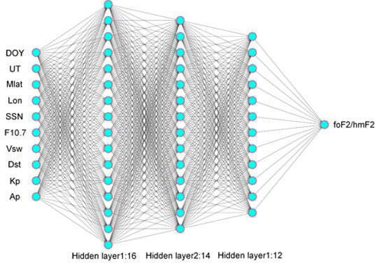
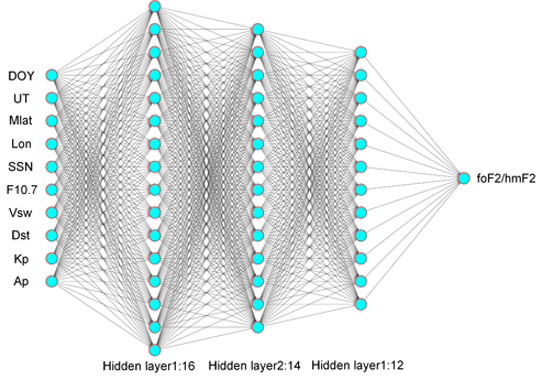
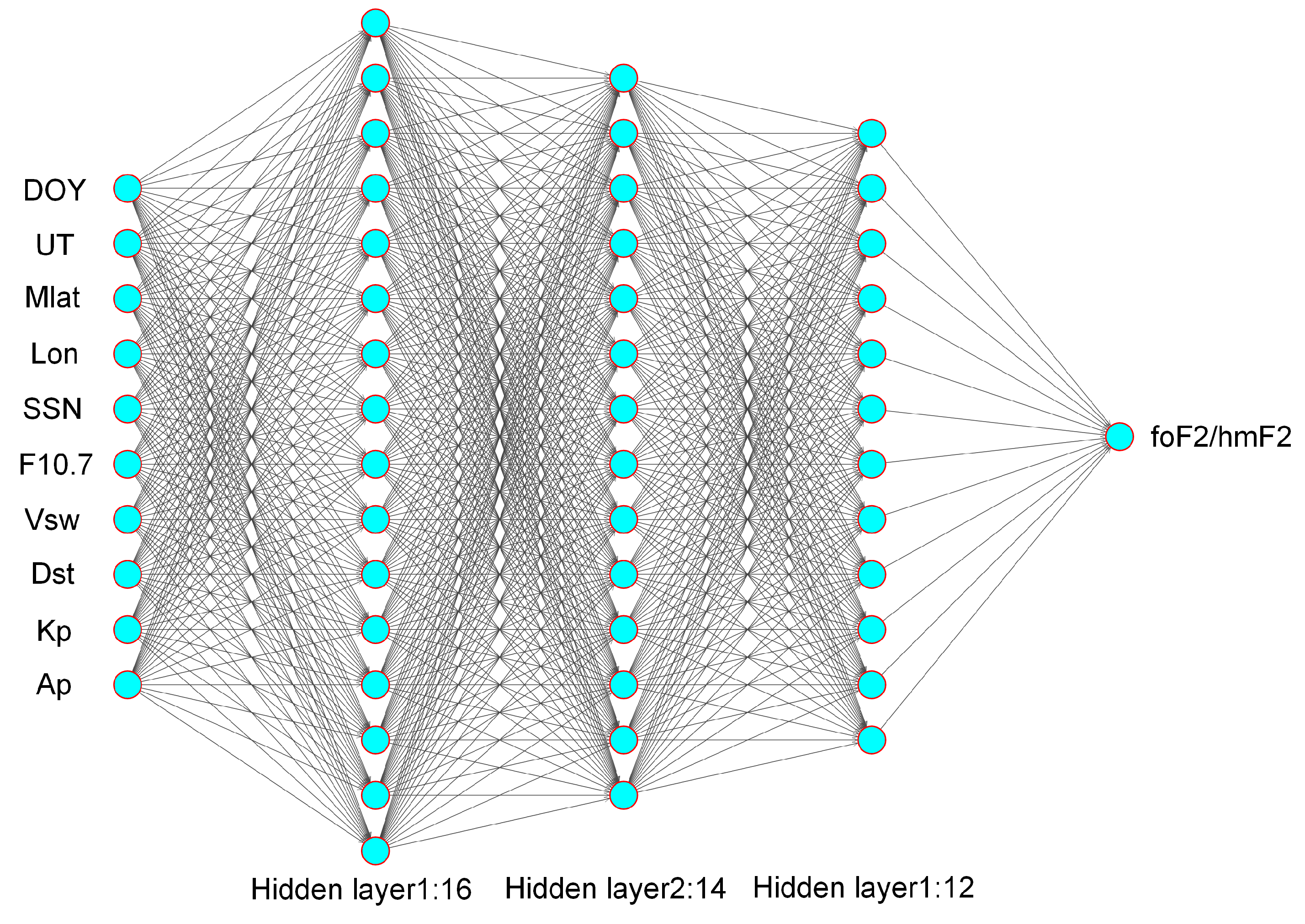
Ten input parameters (same as the input layer in Figure 2) of ionosonde foF2 points IONO_foF2 were taken as the input information for the COSPF and IONOPF models, respectively.

(2).

The foF2 values were simulated by the COSPF and IONOPF models, respectively, namely, COSPF_foF2 and IONOPF_foF2; then, the difference was computed between COSPF_foF2 and IONOPF_foF2.

(3).

The sum of the pre-corrected ionosonde foF2 value IONO_foF2 and the above difference was regarded as the final corrected value COSMIC-foF2corr.

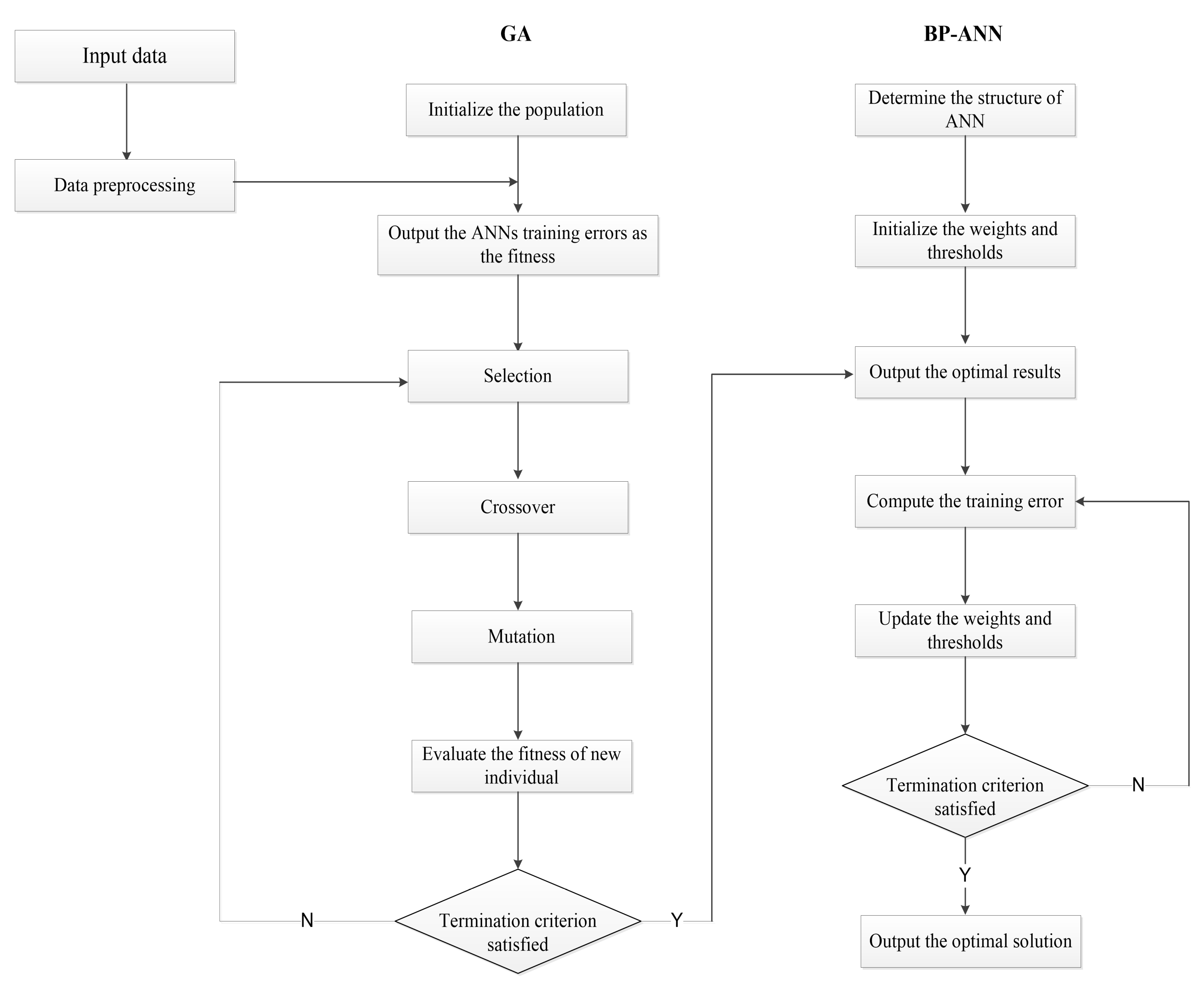
For more details about the correction process, please refer to the following equation:

$$\{\begin{array}{c}COSMIC-foF{2}_{corr}=Ion{o}_{foF2}+COSP{F}_{foF2}-IONOP{F}_{foF2}\\ COSMIC-hmF{2}_{corr}=Ion{o}_{hmF2}+COSP{H}_{hmF2}-IONOP{H}_{hmF2}\\ Iono-foF{2}_{corr}=COSMI{C}_{foF2}-COSP{F}_{foF2}+IONOP{F}_{foF2}\\ Iono-hmF{2}_{corr}=COSMI{C}_{hmF2}-COSP{H}_{hmF2}+IONOP{H}_{hmF2}\end{array}$$

(2)

The results showed that the RMSEs of ionospheric foF2 model developed by uncorrected “mixed” data ranged from 1.2 MHz to 1.4 MHz during four seasons. After data correction, the averaged RMSE of ionospheric model based on the “mixed” corrected data decreased to 0.79 MHz with the negative ratio of 38.3%, especially in the summer, the averaged RMSE reached to 0.68 MHz. Similar to foF2, the RMSEs of hmF2 models developed by “mixed” uncorrected data during four seasons were about 28–32 km, and the corresponding RMSEs based on corrected data ranged from 19.8 km, 22.4 km, 21.5 km and 23.9 km, the maximum descending percent was 29.3%. The comparative results indicated the proposed method was efficient to improve the accuracy of ionospheric models based on the “mixed” COSMIC and ionosonde measurements significantly.

2.2. Methods

The ANN is an information processing system which is formed by a large number of simple processing elements known as neurons and has a powerful ability in capturing the nonlinear relationship between input data and output data [28], it has been widely applied in image recognition, data classification, modeling etc. Usually a simple neural network consists of three layers, namely, an input layer, hidden layer and output layer. Back propagation algorithm is the most famous method in training neural network, which includes two stages: feed-forward and back-forward [29]. In the feed-forward stage, input parameters are processed by neural network to generate output parameters, then the errors between output parameters and targets are calculated. In the back-forward stage, the simulated errors are transferred from the output layer to input layer, and the input weights are estimated again. In the study, the back-propagation algorithm was utilized to develop ionospheric models by ANN technique for foF2 and hmF2. The gradient descent method was also used in developing ANN models, the training process easily stops when the neural network is caught in the “local minimum” effect. In order to solve this problem, the ANN used in the study was optimized by the genetic algorithm (GA). GA is a method based on natural selection for solving both constrained and unconstrained optimization problems; it has been widely applied in many fields [10,30,31]. The GA in the study was used to optimize the initial weight of the ANN, the detail steps were described as following steps and illustrated in Figure 3.

Step 1: Determine the architecture of the neural network, including the numbers of layers and neurons, and estimate the initial weights and thresholds.

Step 2: Input sample and preprocess data.

Step 3: Initialize the population P, including the crossover scale, crossover frequency P_c, mutation frequency P_m etc.

Step 4: Train the network over the training set of sample data using the initial weights and thresholds, and compute the SSE (sum of squared errors) as the fitness value f.

Step 5: Estimate each individual evaluation function, and choose the individual with largest probability, the individual in the population is evaluated by:

$$P_i=\frac{f_i}{{\sum }_{j=1}^N{f}_j}=\frac{f_i}{f_{sum}}$$

(3)

where P_i and f_i are the selected and fitness probability of the individual i, respectively, and f_sum is the sum value of the fitness in the population.

Step 6: Choose the best ranking individuals to generate the new individuals $G_i^{\prime }$ and $G_j^{\prime }$ from the last generation individuals $G_i$ and $G_{i+1}$.

Step 7: Estimate the fitness value of every new individual and replace the worst population with the new individuals.

Step 8: Repeat the steps 5–7 until exceed the termination criterion.

Step 9: Output the optimal weights as the initial weights of neural network and train the network to optimize the weights for optimal solutions.

In the study, the input parameters of the neural network consisted of day of year (DOY), universal time (UT), geomagnetic latitude (GLAT) and geographic longitude (LON). In addition, ionospheric variation is affected by solar-geomagnetic activity seriously, the parameters represent solar-terrestrial environment were also as the inputs. The parameters SSN (sunspot number), Vsw (solar wind speed) and F107 (10.7cm solar flux) were used to represent the intensity of solar radiation. The values Dst, Kp and Ap were selected to represent geomagnetic environment. Our study found that the neutral wind did not play a great role in improving the accuracy of the ANN model; hence, the meridional wind and zonal wind were not used as the input parameters. This ANN structure contained three hidden layers in the study, and the network was trained for more than thousands of times to search for the optimal simulated results. The RMSE of this ANN was minimum when the numbers of nodes in each hidden layer were 16, 14 and 12, respectively, and the corresponding active functions in these hidden layers were tansig, tansig and sigmoid. The architecture of the ANN is shown in Figure 2. After the input parameters and the structure of ANN model were determined, the entire “mixed” corrected measurements were used to develop the ANN-based ionospheric models wholly. In the study, the input parameters, model’s structure and modeling strategy were different from the ANNIM model in literature [32].

3. Results

The remarkable discrepancies between ionospheric observations obtained from multiple techniques are reduced by the proposed method based on machine learning. Then, the corrected “mixed” measurements are used to develop the Global Ionospheric Peak Frequency Model (GIPFM) and Global Ionospheric Peak Height Model (GIPHM) by ANN optimized by the GA. It is noted that the “mixed” data represent the entire COSMIC measurements and ionosonde observations. In order to validate the accuracies of ANN models, comparisons between GIPFM/GIPHM and the International Reference Ionosphere (IRI) in the solar minimum year (2009) and solar moderate year (2013) were conducted. The version of the IRI model was 2016.

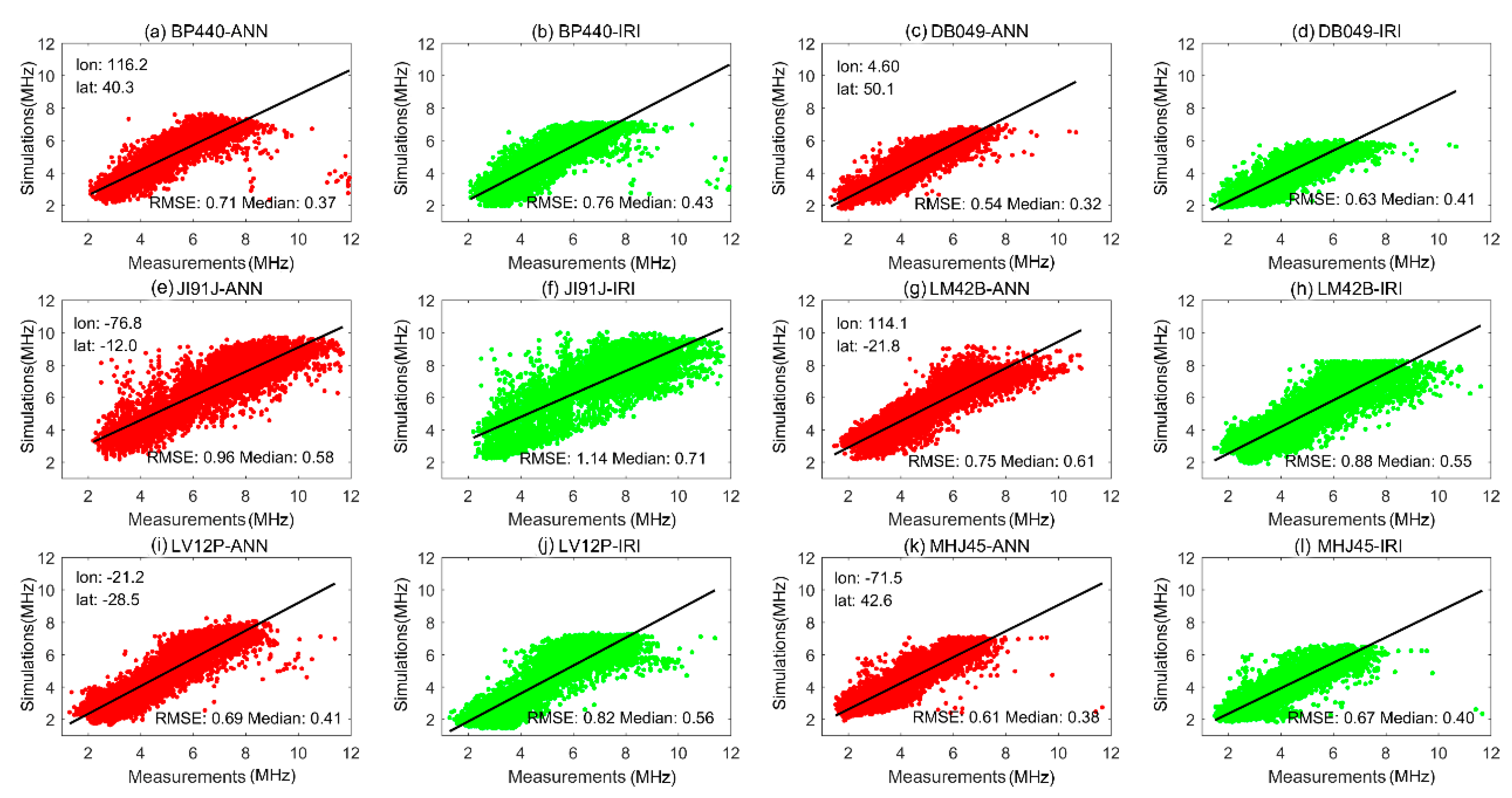
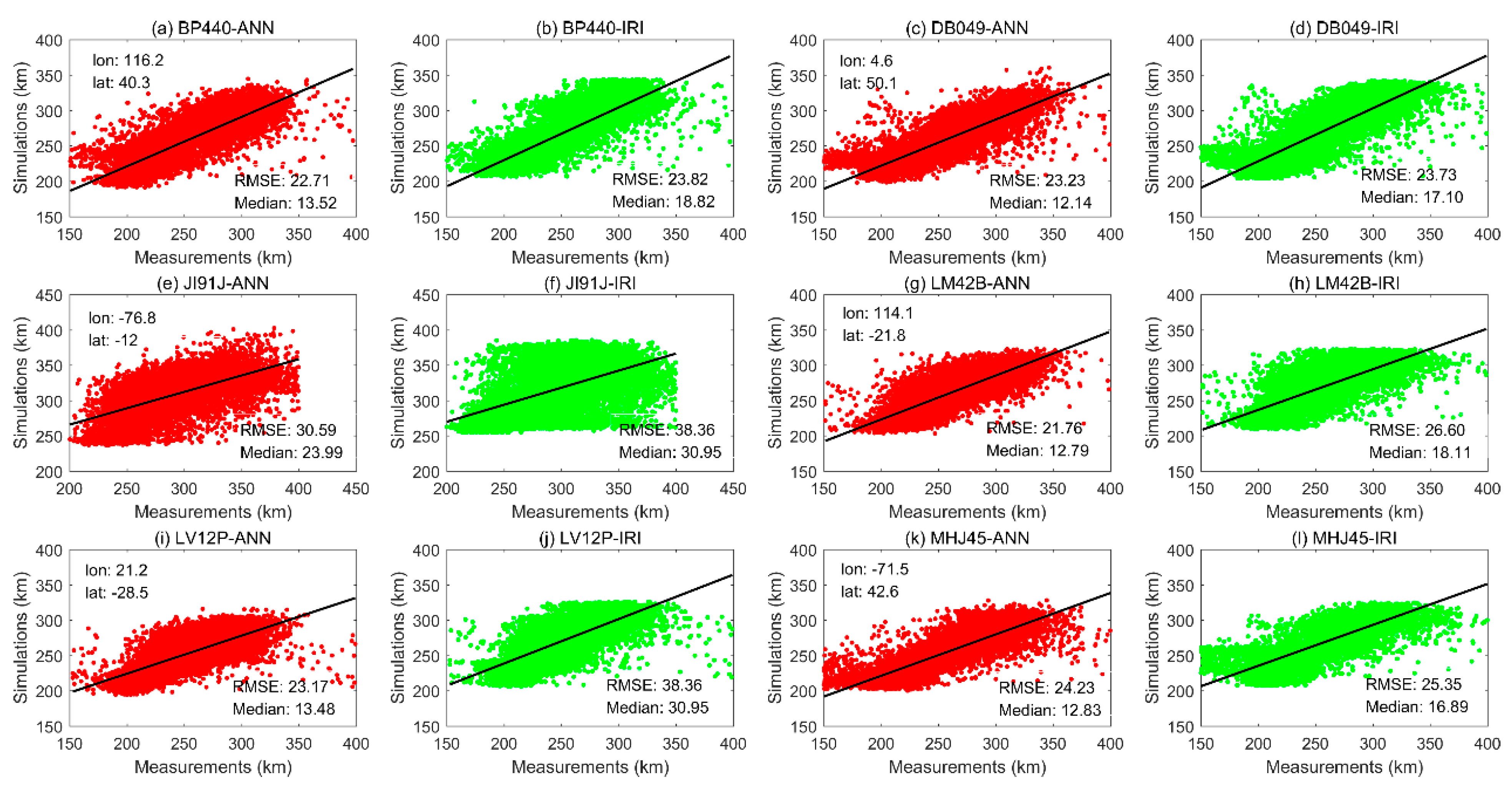
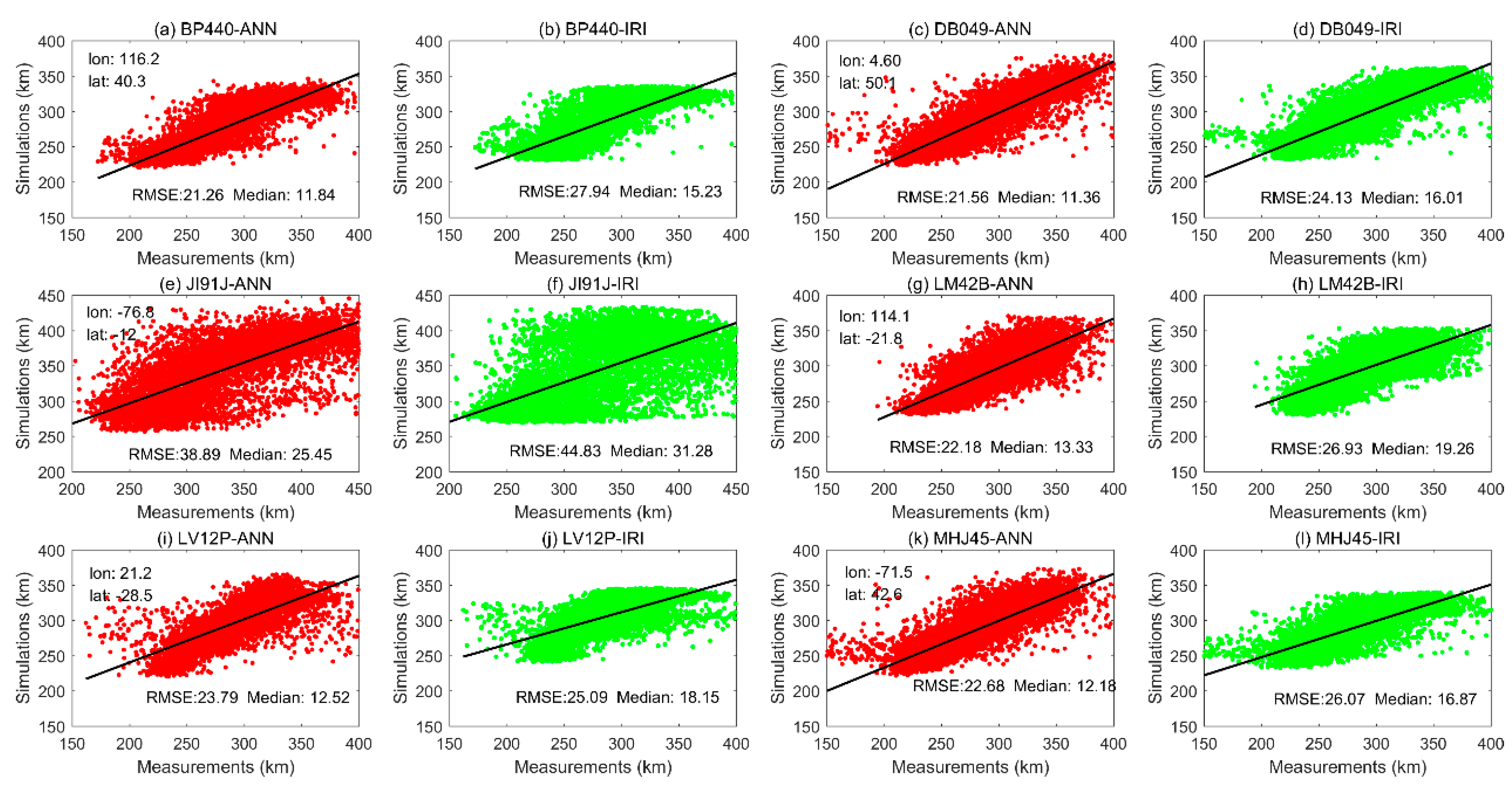
3.1. Validation of Accuracy in the Solar Minimum Year

To evaluate the accuracies of GIPFM and GIPHM in 2009, the observations of ionosonde stations distributed in six continents, excluding Antarctica, were gathered over the entire year. Then, the data sets were extracted from the total observations randomly; each data set contained 10,000 points. Therefore, the selected points were not equally distributed among all seasons and all local times. It was noted that the data set extraction should be conducted before establishing ionospheric models. After that, the selected points were simulated by the GIPFM/GIPHM and IRI-2016, respectively. The results are shown in Figure 4 and Figure 5.

In Figure 4, the abscissa axis represents the ionosonde measurements, and the vertical axis represents the simulated values. The red and green points are the simulations of the ANN model and IRI, respectively. Generally, the simulations of the ANN model agree well with those of the IRI, but the former correlation was obviously higher than the latter correlation. In 2009, the RMSEs of IRI simulations over six stations were 0.76, 0.63, 1.14, 0.88, 0.82 and 0.67 MHz, while the RMSEs of GIPFM simulations were 0.71, 0.54, 0.96, 0.75, 0.69 and 0.61 MHz, respectively. The GIPGM’s simulated accuracies over six ionosondes improved by 6.58%, 14.28%, 15.79%, 14.77%, 15.85% and 8.96%, respectively. Compared with RMSE, the median errors of GIPFM were smaller than those of IRI with an average rate of more than 20%, except over the station LM42B.

Similar to the results for foF2 in Figure 4, the performances of the GIPHM model also experienced a great improvement, but the improvement was different over different ionosondes. For example, the RMSEs of simulations at low latitudes (Station JI91J, LM42B, and LV12P) decreased from 38.36, 26.60 and 38.36 km (IRI) to 30.59, 21.76 and 23.17 km (GIPHM), with decreasing ratios of 20.26%, 18.33% and 39.6%, respectively. Furthermore, the RMSEs of GIPHM simulations in middle latitudes (Stations BP440, DB049, and MHJ45) were about equal to the simulations of IRI. However, the median errors of GIPHM simulations were lower than those of the IRI results over all six stations. As shown in Figure 5a–l, the median errors of GIPHM simulations were lower than the IRI simulated errors by about 28.16%, 29%, 22.49%, 29.38%, 56.44% and 24.04%. These results indicate that both GIPHM and IRI cannot simulate “questionable” data well (here, questionable data means some points far away from the regression line), but the simulated performances of the ANN model are always better than those of the IRI.

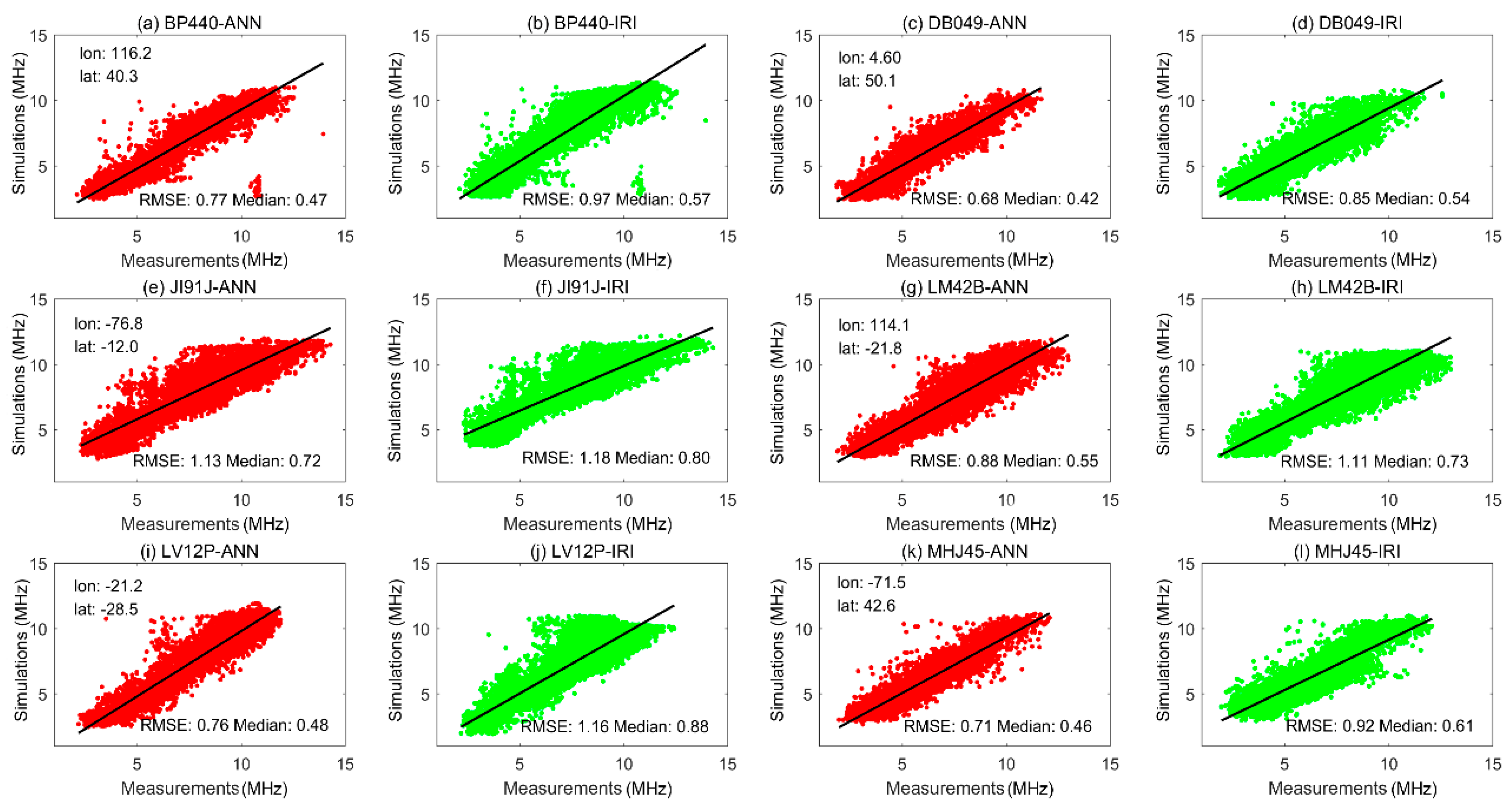
3.2. Validation of Accuracy in the Solar Moderate Year

In a moderate year of solar activity, the simulations of GIPFM agreed well with those of the IRI. In general, the simulated errors of both GIPFM and IRI in 2013 were higher than the errors in 2009, which is associated with the high peak frequency caused by strong solar radiation. The RMSE values of GIPFM simulations were also obviously lower than those of IRI, and the improvement of simulated accuracies in the solar moderate year was more remarkable than that in the solar minimum year. For example, Figure 6 shows that the RMSEs of the IRI simulations over six ionosondes decreased from 0.97, 0.85, 1.18, 1.11, 1.16 and 0.92 MHz to 0.77, 0.68, 1.13, 0.88, 0.76 and 0.71 MHz, following simulations by GIPFM, and the corresponding accuracies improved by about 20.62%, 20%, 4.24%, 20.72%, 34.48% and 22.83%, respectively. The simulated accuracies of GIPFM were 20% higher than IRI over most ionosondes, except in station JI91J, located in the southern crest of the equatorial ionization anomaly (EIA). In the solar moderate year, the ionospheric variation near the geomagnetic equator was very complex and was controlled by many kinds of physical–chemical effects and dynamic processes, such as the fountain effect, eastward electric field, neutral winds etc. It is a great challenge to predict the ionospheric variations near the geomagnetic equator with high accuracy, especially in South America and Southeast Asia.

The RMSEs of GIPHM simulations were also lower than the simulated errors of IRI in the solar moderate year, and the ratios of the six ionosondes were 23.91%, 10.65%, 13.25%, 17.64%, 5.18% and 13%, respectively. The improved accuracy for hmF2 was lower than that for foF2. In Figure 4 and Figure 6, the foF2 values were distributed densely around the regression line, while Figure 7 shows some hmF2 points far away from the regression line, which may have been caused by instrument failure; these points were regarded as “questionable” data. We believe that it is these “questionable” data contribute to the “unsatisfied” performances of GIPHM simulations. The median parameter can represent the “typical” value of a data set, because it is not overly skewed by having a small proportion of extremely large or small values. Figure 7 shows that the median values of hmF2 errors decreased from 15.23, 16.01, 31.28, 19.26, 18.15 and 16.87 km (simulated by IRI) to 11.84, 11.36, 25.45, 13.33, 12.52 and 12.18 km (simulated by GIPHM), with decreasing ratios of 22.26%, 29.04%, 18.64%, 30.79%, 31.02% and 27.80%, respectively. The performance of the median error was much more remarkable than that of the RMSE. Therefore, we believe the GIPHM could improve the hmF2 prediction under a strong solar radiation environment with an accuracy of more than 20% on a global scale.

3.3. Validation of Accuracy over the Greenwich Meridian

In addition to global spatiotemporal variations, the ionosphere also contains several prominent regional anomalies, such as the equatorial ionization anomaly and the Weddell Sea anomaly. These regional anomalies have strong latitudinal characteristics. In order to evaluate the simulated performance of an ANN model dependent on the geographic latitude, the simulated maps of the ANN and IRI models were compared with the reference product along the reference meridian. In this study, the Greenwich meridian was selected as the reference meridian, and the products obtained from the Pushkov Institute of Terrestrial Magnetism, Ionosphere and Radiowave Propagation of the Russian Academy of Sciences (IZMIRAN) were selected as the reference maps. IZMIRAN takes the hourly global ionospheric map (GIM) as an input to the IRI-plas (International Reference Ionosphere model extended to the plasmasphere) to obtain more realistic scale parameters from foF2 and hmF2. The global foF2 and hmF2 maps provided by IZMIRAN can be regarded as new GIM-TEC products [32]. The GIM-TECs are estimated by the dual-frequency observations obtained from hundreds of International GNSS Service (IGS) stations with spherical harmonics and have been widely applied in scientific research and practical productions [33,34,35,36]. Therefore, the IZMIRAN maps were capable of meeting the requirements of this study. Here, the peak parameters’ time series simulated by ANN and IRI were compared with the IZMIRAN product during 2010–2017. The difference was calculated by the ANN/IRI time series minus the reference values. The comparative results are shown in Figure 8.

In Figure 8, the left and right columns indicate the comparative results of foF2 and hmF2, respectively. The panels in the left column indicate that both simulated maps of ANN and IRI agree well with the reference maps. During 2010–2017, the maximum value of ionospheric foF2 along the Greenwich meridian increased from 10 MHz (2010) to 14 MHz (2015). After that, the maximum value gradually decreased to 6–10 MHz, which was associated with the intensity of solar radiation. In addition, both models showed the ability to simulate the ionospheric prominent phenomenon, equatorial ionization anomaly, as two high foF2 crests were distributed at 10°–30°N/S. Figure 8d,e show the differences between ANN/IRI simulations and reference maps. The differential results indicate that there are some discrepancies between simulations and observations, and the discrepancies are dependent on time and latitude. As shown in Figure 8e, the ANN simulations generally produce lower measurements than IZMIRAN in the low latitude area. Most negative differences appear in 2014–2015 with a maximum amplitude of −3 MHz. Moreover, in the middle-high latitudes, the ANN simulations have periodically larger measurements than IZMIRAN in the winter hemisphere. The maximum amplitude of positive difference is within 2 MHz. Compared with Figure 8d, the difference between IRI simulations and IZMIRAN measurements is more remarkable, and the maximum amplitudes of positive and negative differences exceeded 4 MHz and −4MHz, respectively. The simulated error of the IRI model is 25%–50% larger than that of the ANN model, which is consistent with the simulated results shown in Section 3.1 and Section 3.2. In addition, the simulated error of the IRI model is more expanded than the results of the ANN model.

The right column shows that the simulated hmF2 maps of the ANN and IRI models are consistent with the IZMIRAN measurements. The hmF2 value is inversely proportional to the geographic latitude. The maximum hmF2 value over the geographic equator is over 400 km, which is one to two times larger than that in the high latitudes. Furthermore, the high hmF2 crest extends to the South Pole in December. This phenomenon is in accordance with the physical characteristics of the Weddell Sea anomaly. Figure 8i,j show that there were remarkable discrepancies between hmF2 simulations and reference values. In Figure 8i, the simulated hmF2 maps of the ANN model are periodically larger than the IZMIRAN maps in the summer hemisphere. However, in the winter hemisphere, the simulated value is lower than that of the reference, which is contrary to the foF2 comparative results. The maximum values of positive and negative differences are about 60 km and –80 km, especially in 2013–2015. The results indicate that the performance of the ANN model is inversely proportional to the intensity of the solar radiation. Compared with the results in Figure 8i, the differences between IRI’s simulations and the reference maps are more remarkable, and the maximum amplitudes of positive and negative differences exceed 100 km and −100 km, respectively. The results conclude that the simulated accuracy of the IRI model is 20% lower than the level of the ANN model for hmF2.

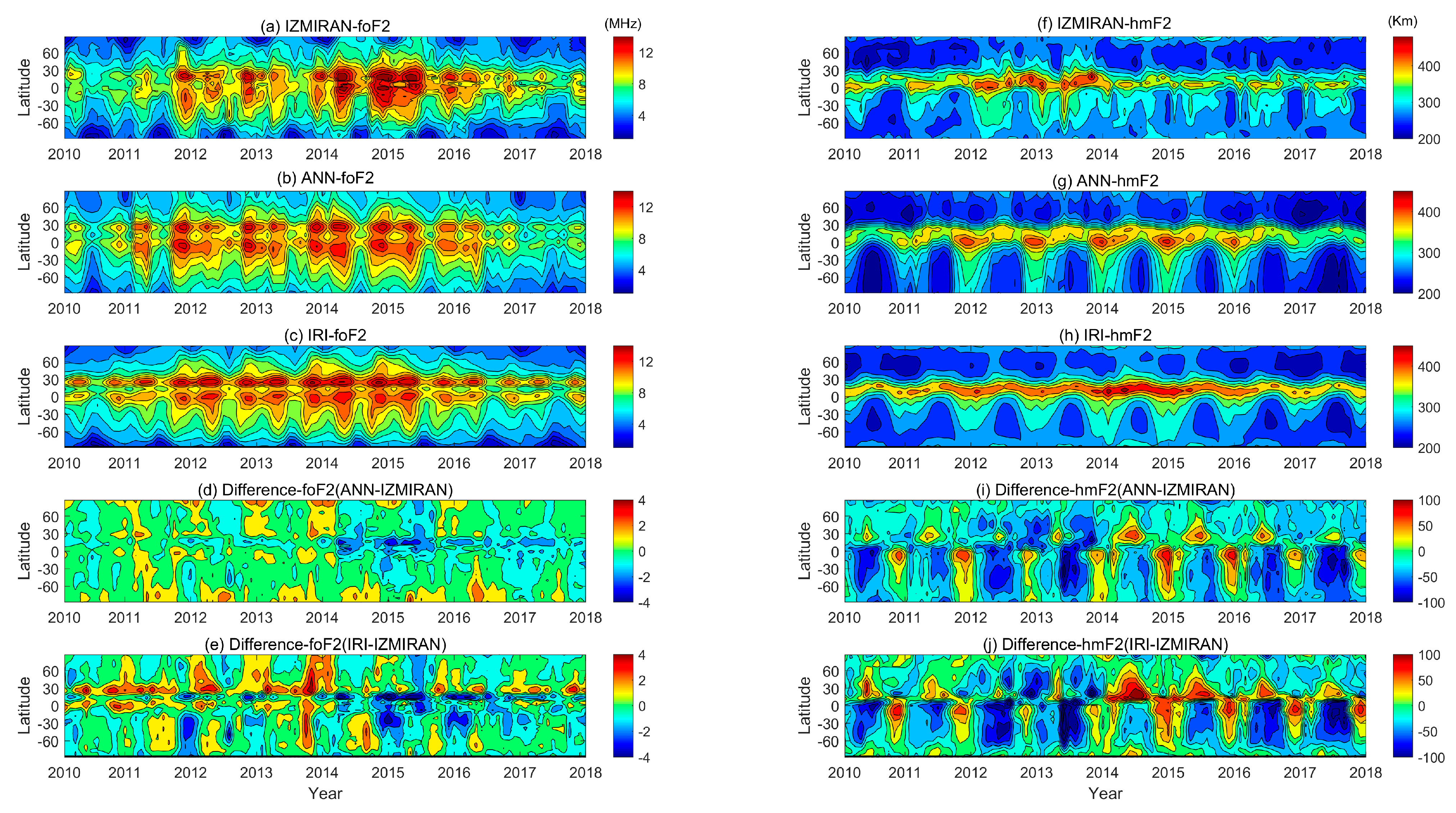
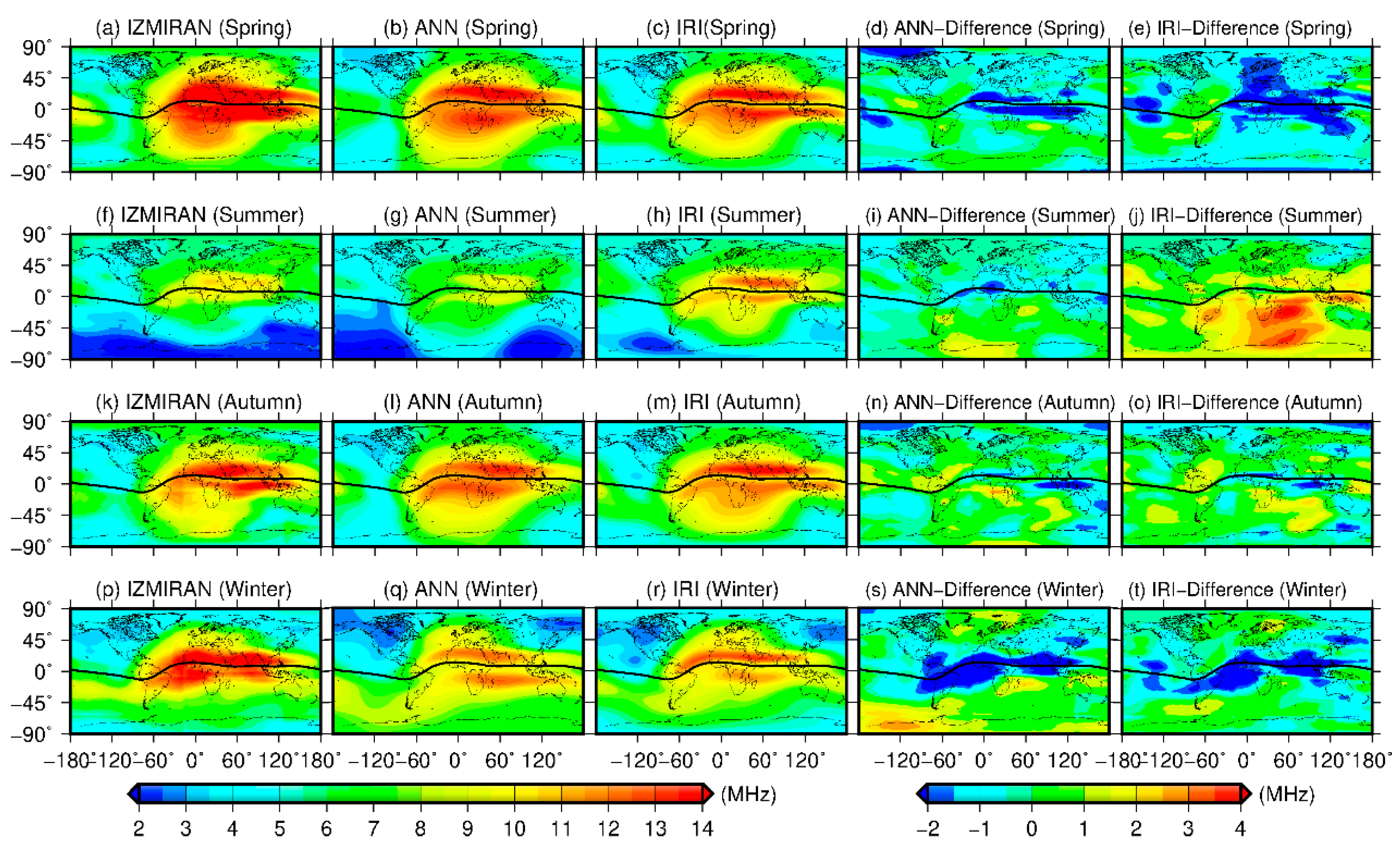
3.4. Validations of Global Spatiotemporal Characteristics

The sections above demonstrate that the ionospheric models developed by the ANN technique provide a great improvement when predicting a peak parameter over a single station or meridian line. Meanwhile, the capability of capturing the global ionospheric spatiotemporal characteristics is also an important criterion for evaluating the performance of ANN models. In this study, the global foF2 and hmF2 maps were simulated by the ANN and IRI models at UT 12:00 in the four seasons of 2014, respectively. It is noted that the days selected in the four seasons were equinoxes and solstices, and the corresponding DOYs (days of year) were 81, 173, 265, and 356. The simulated maps were compared with IZMIRAN measured maps to evaluate the geophysical performances of two models on a global scale. The comparative results are shown in Figure 9 and Figure 10.

The left three columns in Figure 9 represent IZMIRAN measured maps and the foF2 maps simulated by the ANN and IRI models, respectively. The global foF2 maps simulated by ANN and IRI models agree well with the reference values. Both models have the ability to capture the ionospheric spatiotemporal characteristics. The ionospheric foF2 value in the sunlit hemisphere is two to three times larger than that in the night-time hemisphere, and the foF2 value is proportional to the geographic latitude, which is associated with the intensity of solar radiation. In addition, both models are capable of simulating the prominent regional ionospheric features, such as equatorial ionization anomaly, Weddell Sea anomaly etc. The right two columns indicate the differences between the ANN/IRI simulated maps and IZMIRAN measurements. Generally, the simulated performances of the ANN model in the summer solstice and autumn equinox are much better than those in the spring equinox and winter solstice. In summer and autumn, the amplitude of the simulated error of the ANN model ranges from −1 to 1 MHz, while in spring and winter, the simulated foF2 of the ANN model is lower than the reference value in most regions, especially in the regions near the geomagnetic equator. The maximum amplitude of simulated error exceeds −2 MHz. Compared with ANN’s simulations, the simulated errors of the IRI model are larger, not only in the magnitude, but also in the scope. In spring and winter, the simulated values of the IRI model are usually smaller than those of the references, and the negative differences are mainly distributed in Africa, Europe, the Pacific and Western Australia with a maximum amplitude of more than −2 MHz (see Figure 9e,t). Additionally, the simulated errors of the IRI model in the summer solstice were not consistent with the ANN model. The values of IRI’s simulated maps are much larger than the references in the southern hemisphere. Most simulated errors appear in the Indian Ocean with a magnitude of 4 MHz, while the simulated errors of the ANN model are smaller than 1 MHz over the same region at the same time. Therefore, the comparative results in Figure 9 prove that the ionospheric foF2 model developed by the ANN technique not only has a strong ability to capture the ionospheric spatiotemporal characteristics but also improves the simulated accuracy of global ionosphere significantly.

Similar to foF2, the global hmF2 maps simulated by ANN and IRI models were compared with IZMIRAN products, and the results are shown in Figure 10. From the left three columns, it can be seen that the simulated maps are consistent with the reference maps. In the sunlit hemisphere, the ionospheric peak height is proportional to the geographic latitude, and the hmF2 over the geomagnetic equator is one to two times larger than that in the polar regions. While the hmF2 crests gradually move to higher latitude regions in the night, the two crests are distributed within 40°–60°N/S latitudes in the night-time hemisphere. The right two columns show the differences between ANN/IRI’s simulations and reference maps, respectively. In the spring equinox, autumn equinox and winter solstice, the simulated hmF2 values of the ANN model are generally higher than the measured heights in the low–middle latitude areas. The maximum hmF2 differences appear in Africa and the southern Pacific with a magnitude of 40–60 km. However, in the summer solstice (see Figure 10i), ANN’s simulated maps have much lower values than IZMIRAN’s values with magnitudes ranging from −20 to −60 km; especially over the oceans of the southern hemisphere and Antarctica, where the maximum difference exceeds −60 km. The panels in the right column indicate that the differences between IRI’s simulations and references are larger than those of the ANN model in the equinoxes (see Figure 10e,o). The positive differences are mainly distributed in Africa, Southeast Asia and the southern Pacific with a maximum magnitude that exceeds 80 km. However, IRI’s simulated maps are in better agreement with the measured maps than ANN’s performances in the summer solstice, and the IRI’s simulated errors during this period are within −40 to 40 km, which is different from the simulated performances of the GIPFM model at the same time.

4. Discussion

In Section 3, the ANN technique shows a powerful capacity and capability to capture ionospheric spatiotemporal characteristics, and the genetic algorithm was able to improve the learning efficiency of the proposed neural network approach significantly. In the study, the learning efficiencies of the ANN approach were also evaluated with and without the application of the GA method. Thousands of experiments showed that the ANN technique optimized by the GA method can improve the learning efficiency and decrease the simulated error remarkably. The average period of linear regressions optimized by the GA method was 32.7 min with RMSEs of 0.92 MHz for foF2 and 23.7 km for hmF2, while the averaged linear regression without the GA method took about 46.2 min with RMSEs of 1.16 MHz for foF2 and 31.2 km for hmF2, respectively. The comparative results indicate that the learning efficiency of linear regression optimized by GA improves by about 29.22%, and the simulated errors for foF2 and hmF2 decrease by about 20.69% and 24.04%. Therefore, the results demonstrate that the GA method could improve the performance in ionospheric modeling by the ANN technique significantly, which may be a promising tool for further ionospheric studies based on machine learning.

The proposed method used to reduce the discrepancies between multiple instrument measurements shows a strong ability to improve the ionospheric model’s accuracy. In previous studies, many researchers focused on ionospheric modeling based on deep learning with GNSS space-borne occultations or ground-based observations [15,17,24]. In the literature [15], the measurements obtained from 59 ionosondes were used to develop the global foF2 model by a feed-forward neural network. The averaged RMSE values in the solar moderate activity and solar minimum activity were 1.112 MHz and 0.807 MHz, respectively, which are larger than the RMSEs in the corresponding periods (0.82 MHz and 0.71 MHz) in this study. In addition, due to the limitation of geographic distribution of the selected stations, this model fails to capture the ionospheric peak parameters information over the ocean exactly. In order to solve the problem, a previous study [17] multiplied the instrument’s measurements to build the improved ionospheric model ANNIM, such as COSMIC, CHAMP, GRACE and ionosonde. This model was shown represent global ionospheric spatiotemporal characteristics well, but the RMSEs in the solar maximum year (2002) and solar minimum year (2009) for NmF2 were 3.4 × 105 electrons/cm³ and 1.5 × 105 electrons/cm³, and the corresponding RMSEs for hmF2 were 29 km and 25 km, respectively. The RMSE values were much larger than the simulated RMSEs for GIPFM and GIPHM in our study. Many studies have demonstrated that the use of multiple measurements is very helpful to enhance the physical features of ionospheric models, but the technical standard of each measurement is different, and the remarkable discrepancies between different measurements may affect the performance of ionospheric models. This study demonstrates that the proposed method is capable of reducing the discrepancies between multiple measurements and improving the accuracy of the ionospheric model significantly. It is believed that data correction will be an important step in further ionospheric modeling.

5. Conclusions

In this study, a new method based on deep learning method was proposed to reduce the remarkable discrepancies between multiple instrument measurements, such as space-borne COSMIC radio occultation and a ground-based ionosonde. The results show that this method is very helpful for improving the performances of ionospheric models. Then, the “mixed” corrected data (COSMIC and ionosonde) were utilized to develop the ionosphere models for the predictions of foF2 and hmF2 using an artificial neural network optimized by the genetic algorithm, namely, GIPFM and GIPHM. The results indicate that the genetic algorithm could improve the learning efficiency of the proposed neural network approach significantly. The learning efficiency of a linear regression method optimized by the genetic algorithm improved by about 29.22% compared with the experiments without the application of the genetic algorithm. In addition, the above steps also improve the accuracy of the ionospheric model. The accuracy of GIPFM and GIPHM was compared with that of the IRI-2016 model in the solar minimum year (2009) and solar moderate year (2013), respectively. The RMSEs of GIPFM in 2009 and 2013 were about 0.71 MHz and 0.82 MHz, respectively. Both RMSEs were smaller than those of the IRI-2016 model. Especially in a moderate year of solar activity, the simulated performance of the ANN model improved by about 20%–34%. Due to some “questionable” data in the hmF2 sample, the RMSEs of GIPHM did not decrease significantly compared with IRI’s simulations. However, the simulated median errors of GIPHM were still smaller than those of the IRI over the six ionosondes. The improvement in the GIPHM’s accuracy ranged from 20% to 50%. The model validation demonstrates that the GIPFM and GIPHM models developed by the ANN approach are useful for predicting ionospheric foF2 and hmF2 with a higher accuracy.

The performances of the GIPFM and GIPHM models were also compared with the products of IRI and IZMIRAN to evaluate the capability for capturing ionospheric spatiotemporal characteristics. The comparative results indicate that the foF2 and hmF2 maps simulated by the ANN model are in better agreement with the reference values than IRI’s products. In the Greenwich meridian, the differences between GIPFM’s foF2 values and references ranged from −3 MHz to 2 MHz during 2010–2017, and the GIPFM’s simulated error was 25%–50% lower than IRI’s results. Contrary to foF2’s results, for hmF2, the simulated performances of GIPHM were inversely proportional to the intensity of solar radiation. The GIPHM’s simulations were periodically larger than IZMIRAN’s values in the summer hemisphere, while the opposite phenomenon occurred in the winter hemisphere. The amplitudes of negative and positive differences ranged from −80 km to 60 km, which is 20% lower than IRI’s errors. In addition, the ANN models showed a powerful capability to capture ionospheric characteristics, not only global spatiotemporal variations but also some prominent regional anomalies, such as the equatorial ionization anomaly and Weddell Sea anomaly. Furthermore, the global simulated errors of the ANN models were significantly smaller than those of IRI’s simulations. For foF2, the GIPFM’s simulations were generally smaller than those of the references throughout the whole year with an amplitude of −2 MHz to 1 MHz. Especially in the summer solstice and autumn equinox, the model’s performance was much better than the IRI’s with the maximum simulated error exceeding 4 MHz. For hmF2, the GIPHM’s performance was better than the IRI’s on the equinoxes, not only in terms of the simulated accuracy, which improved by about 20%–50%, but also in terms of the scope of the simulated error, which was smaller. However, in the solstices, the GIPHM’s results were not satisfied. Especially in the summer solstice, the simulated errors were mainly distributed in the oceans of the southern hemisphere and Antarctica with the maximum amplitude exceeding −60 km. The simulated errors were two to three times larger than those of the IRI simulation in this region.

This study concludes that the performance of GIPFM and GIPHM developed by the ANN technique optimized by the GA is better than those of previous models, and these models have a high capacity/capability to capture the global or regional ionospheric spatiotemporal characteristics. Therefore, the approach proposed in this study should be extended to more application fields. In further analyses, the global GNSS radio occultations obtained from FORMOSAT-3/COSMIC, the upcoming FORMOSAT-7/COSMIC-2 and the ground-based Digisonde data can be used to develop a complete three-dimensional electron density model by the ANN technique [37].

References

1. Chu, X.; Bortnik, J.; Li, W.; Ma, Q.; Denton, R.; Yue, C.; Angelopoulos, V.; Thorne, R.; Darrouzet, F.; Ozhogin, P. A neural network model of three-dimensional dynamic electron density in the inner magnetosphere. J. Geophys. Res. Space Phys. 2017, 122, 9183–9197. [Google Scholar] [CrossRef]
2. Wichaipanich, N.; Hozumi, K.; Supnithi, P.; Tsugawa, T. A comparison of neural network-based predictions of foF2 with the IRI-2012 model at conjugate points in southeast asia. Adv. Space Res. 2017, 59, 2934–2950. [Google Scholar] [CrossRef]
3. Athieno, R.; Jayachandran, P.; Themens, D. A neural network-based foF2 model for a single station in the polar cap. Radio Sci. 2017, 52, 784–796. [Google Scholar] [CrossRef]
4. Kumluca, A.; Tulunay, E.; Topalli, I.; Tulunay, Y. Temporal and spatial forecasting of ionospheric critical frequency using neural networks. Radio Sci. 1999, 34, 1497–1506. [Google Scholar] [CrossRef]
5. Yue, X.; Wan, W.; Liu, L.; Ning, B.; Zhao, B. Applying artificial neural network to derive long-term foF2 trends in the Asia/Pacific sector from ionosonde observations. J. Geophys. Res. Space Phys. 2006, 111. [Google Scholar] [CrossRef] [Green Version]
6. Hoque, M.; Jakowski, N. A new global model for the ionospheric F2 peak height for radio wave propagation. In Annales Geophysicae; Copernicus GmbH: Göttingen, Germany, 2012; pp. 797–809. [Google Scholar]
7. Zhao, X.; Ning, B.; Liu, L.; Song, G. A prediction model of short-term ionospheric foF2 based on AdaBoost. Adv. Space Res. 2014, 53, 387–394. [Google Scholar] [CrossRef]
8. Oyeyemi, E.O.; McKinnell, L.; Poole, A. Near-real time foF2 predictions using neural networks. J. Atmos. Sol.-Terr. Phys. 2006, 68, 1807–1818. [Google Scholar] [CrossRef]
9. Barkhatov, N.; Revunov, S.; Uryadov, V. Artificial neural network technique for predicting the critical frequency of the ionospheric F 2 layer. Radiophys. Quantum Electron. 2005, 48, 1–13. [Google Scholar] [CrossRef]
10. Wang, R.; Zhou, C.; Deng, Z.; Ni, B.; Zhao, Z. Predicting foF2 in the China region using the neural networks improved by the genetic algorithm. J. Atmos. Sol.-Terr. Phys. 2013, 92, 7–17. [Google Scholar] [CrossRef]
11. Williscroft, L.A.; Poole, A.W. Neural networks, foF2, sunspot number and magnetic activity. Geophys. Res. Lett. 1996, 23, 3659–3662. [Google Scholar] [CrossRef]
12. McKinnell, L.; Oyeyemi, E. Equatorial predictions from a new neural network based global foF2 model. Adv. Space Res. 2010, 46, 1016–1023. [Google Scholar] [CrossRef]
13. Xenos, T. Neural-network-based prediction techniques for single station modeling and regional mapping of the foF2 and M (3000) F2 ionospheric characteristics. Nonlinear Process. Geophys. 2002, 9, 477–486. [Google Scholar] [CrossRef] [Green Version]
14. McKinnell, L.-A.; Friedrich, M. A neural network-based ionospheric model for the auroral zone. J. Atmos. Sol.-Terr. Phys. 2007, 69, 1459–1470. [Google Scholar] [CrossRef]
15. Oyeyemi, E.; Poole, A.; McKinnell, L. On the global model for foF2 using neural networks. Radio Sci. 2005, 40. [Google Scholar] [CrossRef]
16. Liu, J.-Y.; Lin, C.; Lin, C.; Tsai, H.; Solomon, S.; Sun, Y.; Lee, I.; Schreiner, W.; Kuo, Y. Artificial plasma cave in the low-latitude ionosphere results from the radio occultation inversion of the FORMOSAT-3/COSMIC. J. Geophys. Res. Space Phys. 2010, 115. [Google Scholar] [CrossRef]
17. Tulasi Ram, S.; Sai Gowtam, V.; Mitra, A.; Reinisch, B. The Improved Two-Dimensional Artificial Neural Network-Based Ionospheric Model (ANNIM). J. Geophys. Res. Space Phys. 2018, 123, 5807–5820. [Google Scholar] [CrossRef]
18. Krankowski, A.; Zakharenkova, I.; Krypiak-Gregorczyk, A.; Shagimuratov, I.I.; Wielgosz, P. Ionospheric electron density observed by FORMOSAT-3/COSMIC over the European region and validated by ionosonde data. J. Geod. 2011, 85, 949–964. [Google Scholar] [CrossRef] [Green Version]
19. McNamara, L.F.; Thompson, D.C. Validation of COSMIC values of foF2 and M (3000) F2 using ground-based ionosondes. Adv. Space Res. 2015, 55, 163–169. [Google Scholar] [CrossRef]
20. Ely, C.; Batista, I.; Abdu, M. Radio occultation electron density profiles from the FORMOSAT-3/COSMIC satellites over the Brazilian region: A comparison with Digisonde data. Adv. Space Res. 2012, 49, 1553–1562. [Google Scholar] [CrossRef]
21. Sun, L.; Zhao, B.; Yue, X.a.; Mao, T. Comparison between ionospheric character parameters retrieved from FORMOSAT3 measurement and ionosonde observation over China. Chin. J. Geophys. 2014, 57, 3625–3632. [Google Scholar]
22. Hoque, M.; Jakowski, N. A new global empirical NmF2 model for operational use in radio systems. Radio Sci. 2011, 46, 1–13. [Google Scholar] [CrossRef]
23. Bilitza, D.; Reinisch, B.W.; Radicella, S.M.; Pulinets, S.; Gulyaeva, T.; Triskova, L. Improvements of the International Reference Ionosphere model for the topside electron density profile. Radio Sci. 2006, 41. [Google Scholar] [CrossRef]
24. Gowtam, V.S.; Ram, S.T. An Artificial Neural Network-Based Ionospheric Model to Predict NmF2 and hmF2 Using Long-Term Data Set of FORMOSAT-3/COSMIC Radio Occultation Observations: Preliminary Results. J. Geophys. Res. Space Phys. 2017, 122, 11743–11755. [Google Scholar] [CrossRef]
25. Chu, Y.-H.; Su, C.-L.; Ko, H.-T. A global survey of COSMIC ionospheric peak electron density and its height: A comparison with ground-based ionosonde measurements. Adv. Space Res. 2010, 46, 431–439. [Google Scholar] [CrossRef]
26. Hu, L.; Ning, B.; Liu, L.; Zhao, B.; Chen, Y.; Li, G. Comparison between ionospheric peak parameters retrieved from COSMIC measurement and ionosonde observation over Sanya. Adv. Space Res. 2014, 54, 929–938. [Google Scholar] [CrossRef]
27. Lei, J.; Syndergaard, S.; Burns, A.G.; Solomon, S.C.; Wang, W.; Zeng, Z.; Roble, R.G.; Wu, Q.; Kuo, Y.H.; Holt, J.M. Comparison of COSMIC ionospheric measurements with ground-based observations and model predictions: Preliminary results. J. Geophys. Res. Space Phys. 2007, 112. [Google Scholar] [CrossRef]
28. Haykin, S. Neural Networks: A Comprehensive Foundation; Prentice Hall: Upper Saddle River, NJ, USA, 1994. [Google Scholar]
29. Razin, M.; Voosoghi, B. Regional application of multi-layer artificial neural networks in 3-D ionosphere tomography. Adv. Space Res. 2016, 58, 339–348. [Google Scholar] [CrossRef]
30. Montana, D.J.; Davis, L. Training Feedforward Neural Networks Using Genetic Algorithms. In Proceedings of the IJCAI, Detroit, MI, USA, 20–25 August 1989; pp. 762–767. [Google Scholar]
31. Song, R.; Zhang, X.; Zhou, C.; Liu, J.; He, J. Predicting TEC in China based on the neural networks optimized by genetic algorithm. Adv. Space Res. 2018, 62, 745–759. [Google Scholar] [CrossRef]
32. Gulyaeva, T. Storm time behavior of topside scale height inferred from the ionosphere–plasmasphere model driven by the F2 layer peak and GPS-TEC observations. Adv. Space Res. 2011, 47, 913–920. [Google Scholar] [CrossRef]
33. Li, W.; Yue, J.; Yang, Y.; He, C.; Hu, A.; Zhang, K. Ionospheric and Thermospheric Responses to the Recent Strong Solar Flares on 6 September 2017. J. Geophys. Res. Space Phys. 2018, 123, 8865–8883. [Google Scholar] [CrossRef] [Green Version]
34. Li, W.; Yue, J.; Wu, S.; Yang, Y.; Li, Z.; Bi, J.; Zhang, K. Ionospheric responses to typhoons in Australia during 2005–2014 using GNSS and FORMOSAT-3/COSMIC measurements. GPS Solut. 2018, 22, 61. [Google Scholar] [CrossRef]
35. Li, W.; Yue, J.; Guo, J.; Yang, Y.; Zou, B.; Shen, Y.; Zhang, K. Statistical seismo-ionospheric precursors of M7. 0+ earthquakes in Circum-Pacific seismic belt by GPS TEC measurements. Adv. Space Res. 2018, 61, 1206–1219. [Google Scholar] [CrossRef]
36. Du, W.; Liu, X.; Guo, J.; Shen, Y.; Li, W.; Chang, X. Analysis of the melting glaciers in Southeast Tibet by ALOS-PALSAR data. Terr. Atmos. Ocean. Sci. 2019, 30, 1–13. [Google Scholar] [CrossRef] [Green Version]
37. Yue, X.; Schreiner, W.S.; Pedatella, N.; Anthes, R.A.; Mannucci, A.J.; Straus, P.R.; Liu, J.Y. Space weather observations by GNSS radio occultation: From FORMOSAT-3/COSMIC to FORMOSAT-7/COSMIC-2. Space Weather 2014, 12, 616–621. [Google Scholar] [CrossRef] [PubMed] [Green Version]
Figure 1. Daily averaged F10.7 and the numbers of COSMIC and ionosonde measurements per month during 2007–2016.
Remotesensing 12 00866 g001
Figure 2. Schematic structure of the artificial neural network
Remotesensing 12 00866 g002
Figure 3. The flowchart of the artificial neural network (ANN) optimized by the genetic algorithm
Remotesensing 12 00866 g003
Figure 4. Various comparisons of the simulated accuracies between the Global Ionospheric Peak Frequency Model (GIPFM) and the International Reference Ionosphere (IRI)-2016 in 2009
Remotesensing 12 00866 g004
Figure 5. Similar to Figure 4, but for hmF2.
Remotesensing 12 00866 g005
Figure 6. Comparison of the accuracies between Global Ionospheric Peak Frequency Model (GIPFM) and International Reference Ionosphere (IRI) in 2013.
Remotesensing 12 00866 g006
Figure 7. Similar to Figure 6, but for hmF2.
Remotesensing 12 00866 g007
Figure 8. Comparative results of foF2 and hmF2 from the Pushkov Institute of Terrestrial Magnetism, Ionosphere and Radiowave Propagation of the Russian Academy of Sciences (IZMIRAN), ANN and IRI along the Greenwich meridian during 2010–2017.
Remotesensing 12 00866 g008
Figure 9. Comparative analysis of global foF2 maps of IZMIRAN, ANN and IRI at noon in four seasons. The black line represents the geomagnetic equator.
Remotesensing 12 00866 g009
Figure 10. Similar to Figure 9, but for hmF2.
Remotesensing 12 00866 g010