Abstract
In this study, an improved geographically and temporally weighted regression (IGTWR) model for the estimation of hourly PM2.5 concentration data was applied over central and eastern China in 2017, based on Himawari-8 Advanced Himawari Imager (AHI) data. A generalized distance based on the longitude, latitude, day, hour, and land use type was constructed. AHI aerosol optical depth, surface relative humidity, and boundary layer height (BLH) data were used as independent variables to retrieve the hourly PM2.5 concentrations at 1:00, 2:00, 3:00, 4:00, 5:00, 6:00, 7:00, and 8:00 UTC (Coordinated Universal Time). The model fitting and cross-validation performance were satisfactory. For the model fitting set, the correlation coefficient of determination (R2) between the measured and predicted PM2.5 concentrations was 0.886, and the root-mean-square error (RMSE) of 437,642 samples was only 12.18 µg/m3. The tenfold cross-validation results of the regression model were also acceptable; the correlation coefficient R2 of the measured and predicted results was 0.784, and the RMSE was 20.104 µg/m3, which is only 8 µg/m3 higher than that of the model fitting set. The spatial and temporal characteristics of the hourly PM2.5 concentration in 2017 were revealed. The model also achieved stable performance under haze and dust conditions.
1. Introduction
Real-time monitoring of ground-level fine particulate matter (PM2.5) concentrations is essential for the early warning of extreme weather events such as dust and haze, and the prediction of health exposure risks [1]. Satellite remote sensing with a large spatial coverage and continuous observations can address the limitations of ground-based monitoring [2,3,4,5] and provide comprehensive and reliable PM2.5 monitoring. Daily monitoring by polar orbit satellites cannot meet the requirements for real-time continuous monitoring. By contrast, the geostationary satellite Himawari-8 can provide high-frequency observations with broad coverage. Several aerosol retrieval methods based on Himawari-8 data have been developed [6,7,8]. Using an optimal estimation method, She et al. [9] successfully retrieved the aerosol optical depth (AOD) from Himawari-8 data, and their algorithm estimated the hourly AOD over land with considerable accuracy.
Several algorithms have been developed to exploit the quantitative relationship between the AOD and PM2.5 concentration, such as a semi-empirical model [10,11,12,13], multiple linear regression model [14], land use regression model [15], linear or nonlinear mixed effects model [16], generalized linear regression model [17], geographically weighted regression (GWR) model [18,19], and geographically and temporally weighted regression (GTWR) model [10]. There are some studies on the estimation of the hourly PM values using Himawari-8 aerosol property data, for example, studies on the estimation of the hourly PM2.5 for the Beijing–Tianjin–Hebei region using a linear mixed-effect model [20] and the hourly PM2.5 concentrations in Hebei using a vertical-humidity correction method [21]. The machine learning algorithm is also used to estimate hourly PM2.5 over China [22,23]. However, research on hourly PM2.5 data estimation for a large region of China based on the traditional statistical models is limited.
The least-squares method and GWR model were used to estimate PM2.5 in the United States [24], over North America [18], and in China [19,25]. The GWR model is significantly more accurate than linear regression models. A GTWR model has been applied to MODIS/AOD data to calculate the ground-level PM2.5 concentrations over China [26]. As the spatial and temporal variations should be considered simultaneously in the estimation of hourly PM2.5 concentration data, a GTWR model is adopted in this study.
The PM monitoring network in China was built in 2012. Although monitoring stations of the network are located across the country, the distribution of the stations is spatially uneven. Most of them are located in central and eastern China, and only a few stations are present in the western part. Therefore, in this study, the hourly PM2.5 data for central and eastern China, where extreme weather events such as haze and dust storms are frequent, were estimated. This paper describes the algorithm for retrieving the hourly PM2.5 concentrations over central and eastern China using AOD data from the geostationary satellite Himawari-8. The selection of input parameters, calculation and setting of the key coefficients of the model, model structure composition, model performance, temporal and spatial distribution of hourly PM2.5, and model testing under extreme weather conditions are also discussed.
2. Study Area and Data Sources
2.1. Study Area
This study focused on estimation of the hourly PM2.5 data over central and eastern China. The study area (Figure 1, red boundary line) is located on the first and second steppes of China and has a varied topography, which increases the uncertainty in the estimation of PM2.5. Therefore, we consider the full impact of the possible factors and select a suitable data set for the establishment of the model.
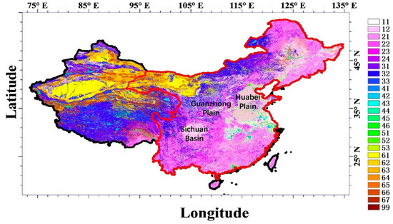
Figure 1.
The distribution of land use types over China in 2015 [27]. The number of different land use types refers to the Land Use and Cover Change (LUCC) classification system, as shown in Table 1. The red boundary line represents the study area.
2.2. Data Sources
2.2.1. PM2.5 Data
The in situ ground-level PM2.5 concentrations are provided by the National Real-time Air Quality Publishing Platform (http://106.37.208.233:20035/). We collected hourly PM2.5 data for 1385 sites in the study area in 2017. The stations are relatively dense in urban areas, especially in the North China Plain, Northeast Plain, Yangtze River Delta, Guanzhong Plain, Pearl River Delta, and Sichuan Basin. The ground-based PM2.5 observation network provides sufficient data to support the construction of the PM2.5 remote sensing estimation model.
2.2.2. Himawari-8 Data
Level 1 (L1) data from the geostationary satellite Himawari-8 are officially provided by Japan’s Meteorological Administration at resolutions of 2 and 5 km (ftp.ptree.jaxa.jp). When the atmospheric conditions remained relatively stable for an hour, we estimated the PM2.5 concentrations hourly. The L1 data used in this study were recorded at 1:00, 2:00, 3:00, 4:00, 5:00, 6:00, 7:00, and 8:00 UTC (Coordinated Universal Time). Himawari-8 Advanced Himawari Imager (AHI) AOD data were obtained using the joint retrieval algorithm for the surface reflectance and aerosol optical thickness proposed and implemented by She et al. [9].
2.2.3. Land Use Type
Notably, the land use types in adjacent areas may be different. For example, there are two different types of cultivated land, paddy fields and dry land, in eastern China. The underlying surface inevitably affects the relationship between the AOD and PM2.5. This study mainly focuses on the effects of geographic distance, the type of underlying surface, the observation time, and other factors. The data on land use types in China in 2015 were provided by the Resource and Environment Data Cloud Platform (http://www.resdc.cn/) at a resolution of 10 km. These data were obtained via remote sensing interpretation methods, with human-computer interactions and visual interpretations based on Landsat 8 data [27]. Figure 1 shows the distribution of land use types in China in 2015. Table 1 describes the Land Use and Cover Change (LUCC) classification system. The land use types show the distribution of arable land, woodland, grassland, and desert from the east to the inland northwestern area.

Table 1.
The land use types of LUCC classification system over China [27].
2.2.4. Relative Humidity
The relative surface humidity in central and eastern China varies greatly between 9:00 a.m. and 16:00 p.m. Beijing time. Atmospheric moisture plays an important role in the formation of secondary pollutants. Therefore, the humidity must be considered in PM estimations. The surface relative humidity data used in this study are derived from Global Surface Summary of the Day observation data (https://catalog.data.gov/dataset/global-surface-summary-of-the-day-gsod). The temporal resolution is 30 min or 3 h depending on the site. First, we performed the temporal interpolation for each site. For each of the eight times from 9:00 a.m. to 16:00 p.m. Beijing time on one site, the closest relative humidity observation data before and after the time were extracted. The linear interpolation between the closed data extracted was used to obtain the relative humidity at each time. Then, we performed the spatial interpolation for each time. The surface relative humidity of each time was obtained via inverse distance-weighted interpolation between all the observation sites.
2.2.5. Boundary Layer Height
The boundary layer height has a notable effect on the atmospheric particulate matter concentrations [28]. The planetary boundary layer height used in this study was obtained from the ERA-2000 dataset released by the European Centre for Medium-Range Weather Forecasts (ECMWF), with a time resolution of 3 h. The BLH data on each site were extracted according to the ECMWF BLH value on its located pixel. The intraday hourly BLH was obtained by the linear interpolation between the closed data before and after each time. The intraday hourly BLH over central and eastern China was obtained via inverse distance-weighted interpolation between all the observation sites.
3. Improved Geographically and Temporally Weighted Regression Model
The geographic data are affected by both spatial and temporal factors. The geographically and temporally weighted regression model (GTWR) has been developed to solve the temporal and spatial problems (Equation (1)) [29]:
In this function, i denotes the observation point (i = 1, 2, ..., n, where n is the total number of observation points), k is a modelling parameter (k = 1, 2, ..., d, where d is the total number of parameters), is the estimated parameter, is the independent variable representing the value of k at point i, and is the coefficient; , , and denote the longitude, latitude, and date, respectively, and represents the random error.
However, the estimation of surface level PM2.5 is not only affected by spatial–temporal factors, but also influenced by the underlying surface conditions. In this study, an improved geographically and temporally weighted regression (IGTWR) model was thereby established (Equation (2)). The parameters used in this model are AOD, RH, and BLH. The spatial (longitude and latitude), temporal (day and hour), and underlying surface data (land use data) are used to characterize the relationship between different sample sites.
Equation (2) can be written as Equation (3):
In Equations (2) and (3), , , , , represent longitude, latitude, day, hour, and land use type, respectively. d refers to the number of independent variables (Himawari-8 AOD, relative humidity, and boundary layer height) in this model, and d = 3; i denotes the observation point, i = 1, 2, ..., n, where n is the total number of observation points.
In this study, in order to calculate the weights of different sites in the regression process, the improved geographical and temporal weights were introduced into the model. The weights were calculated using the longitude, latitude, day, hour, and land use type data for the 1385 observation stations in the study area. The Himawari-8 AOD, relative humidity, and boundary layer height data were used as independent variables to fit the concentration of PM2.5 over the study area. The objective function f is given by
The regression objective is to find a set of coefficients that can minimize the objective function f. Assuming that a set of coefficients can minimize the objective function according to the least-squares principle:
The partial derivative of the objective function f (Equation (4)) is computed, and the partial derivative with , r = 0, 1, …, d, is then set equal to 0, as follows:
Equation (6) can be written as the following equation (Equation (7)):
The next step is to solve the above equations (Equation (7)). Let W, Y, and X represent the following matrices:
Then, Equation (7) can be expressed as follows:
The estimated value, (Equation (13)), of at can be obtained by solving Equation (11) as follows (Equation (12)):
The estimated PM2.5 concentration Y at is as follows:
Therefore, the PM2.5 concentration at is as follows:
and
The selection of the weight coefficient is particularly important for the regression model. The methods of calculating and selecting the weight coefficient are described below.
The distance between the estimated points and any other observed sample data is defined as
Here, , , and are the weight coefficients. The weight function is expressed as a Gaussian function:
Here, , , , and are the bandwidths corresponding to the spatial (longitude and latitude), temporal (day and hour), and land use bandwidths, and , and are weights.
In this study, the cross-validation method [30] is used to select the optimal bandwidth and the optimal bandwidth that can provide the minimum residual:
In this study, we used spatial, temporal, and underlying surface parameters to calculate the weight of different samples in the regression model. The hourly AHI AOD, BLH, and RH were used as independent variables to estimate the hourly surface level PM2.5 over central and eastern China. The tenfold cross-validation was used as the PM2.5 validation method. The model performance in the haze and dust event has also been evaluated and analyzed (Figure 2).
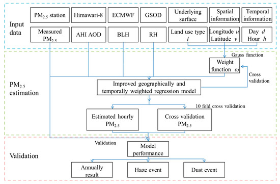
Figure 2.
The model building and analysis strategy of the improved geographically and temporally weighted regression proposed in this study.
4. Results
4.1. Performance Evaluation of the IGTWR Model
In this study, the temporal, geographical, and underlying surface-weighted regression model was used to retrieve the ground-level PM2.5 for 8 h per day during the daytime over central and eastern China in 2017. The hourly Himawari-8 AOD (1:00, 2:00, 3:00, 4:00, 5:00, 6:00, 7:00, and 8:00 UTC, which correspond to 9:00, 10:00, 11:00, 12:00, 13:00, 14:00, 15:00, and 16:00 Beijing time), surface relative humidity, and boundary layer height were selected as input parameters. The longitude, latitude, day, hour, and land use type were used to estimate the regression weight, and 437,642 samples were successfully matched and used as the modelling set to construct the GWR model. The model fitting performance is shown in Figure 3 (left). The tenfold cross-validation method was used to evaluate the model fitting (Rodriguez et al. 2010). We split the 437,642 matched data points evenly into ten parts. One part was used for validation, and the remaining nine parts were used for training. This process was repeated for every fold. The cross-validation results are shown in Figure 3 (right). For the 437,642 samples, the R2 value between the predicted and observed PM2.5 is 0.886, and the root-mean-square error (RMSE) of the model fit is only 12.180 µg/m3. In the scatterplot of the measured values versus the predicted values, the points are distributed around the 1:1 line. The correlation coefficient R2 of the cross-validation is 0.784, and the RMSE is 20.104 µg/m3, which is only 8 µg/m3 higher than the RMSE of the model fit. The slope of the fitting line of the measured–predicted PM2.5 scatter plot is 0.747, which indicates that the PM2.5 was underestimated. However, for most sample points below 200 µg/m3, this underestimation is not obvious. The accuracy, reliability, and robustness of the PM2.5 estimation under typical conditions are relatively high.
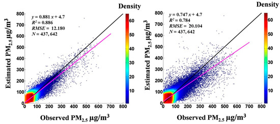
Figure 3.
Scatter plots for (left) model fitting result and (right) tenfold cross-validation result. The color represents the sample density within a 10 µg/m3 radius.
4.2. Hourly PM2.5 Concentration in Central and Eastern China
The hourly spatial distributions of PM2.5 in the central and eastern parts of China are shown in Figure 4. The distribution of the 1385 sites is also shown in Figure 4 (second column from left). In addition, the annual PM2.5 concentrations based on observational data are also shown in Figure 4. The annual average PM2.5 concentration is below 100 µg/m3 for most of the study area. The spatial and temporal patterns of the estimated PM2.5 concentrations are in agreement with the observed patterns.
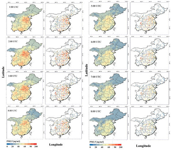
Figure 4.
Annual average hourly PM2.5 concentration in 2017. Columns 1 and 3 are the model estimation results, and columns 2 and 4 are the site observation data (the column number is 1, 2, 3, and 4 from left to right).
Spatially, severe atmospheric fine particulate matter pollution occurred mainly in the North China Plain, the Guanzhong Plain, the Fenwei Plain, the Yangtze River Delta, South China, and the Sichuan Basin. The fine particulate matter pollution in the North China Plain was extreme. An area of relatively stable and severe PM2.5 pollution formed in southern Hebei Province and northern Henan Province at the eastern foot of the Taihang Mountains owing to the effect of the mountains. Notably, the PM2.5 concentration in Beijing is even lower than that in the Yangtze River Delta and Pearl River Delta, which may be related to the air pollution measured in Beijing. The Atmospheric Environment Meteorological Bulletin also showed that the air quality values in Beijing, Tianjin, and Hebei improved continuously in 2017, and the annual number of haze pollution days dropped by 18.1. In southern China, for example, in Guangxi, the annual average concentration of fine particulate matter is more than 40–60 µg/m3. This result may be related to the unfavorable air diffusion conditions, such as temperature inversions, and the effects of biomass combustion in northern China and southern Asia [31].
Temporally, the PM2.5 concentrations in central and eastern China are higher in the morning and lower in the afternoon, and they tend to decrease gradually with time. Figure 4 shows that the highest concentration of PM2.5 occurred at 2:00 UTC. The annual mean concentration of PM2.5 in the main polluted areas is above 60 µg/m3 and then decreases gradually with time. At 8:00 UTC, the average PM2.5 concentration in the main polluted areas falls below 60 µg/m3. This variation in hourly PM2.5 may be closely related to the meteorological conditions. Before sunrise, the height of the atmospheric boundary layer is relatively low, and aerosols are concentrated in the lower level of the atmosphere, which results in a relatively high PM2.5 concentration near the surface. Then, with increasing solar altitude, the atmosphere is heated by solar radiation, which causes expansion and thermodynamic uplift, and the boundary layer rises accordingly [32,33]. The atmospheric particulate matter also moves to the upper atmosphere, resulting in a gradual decrease in the ground-level PM2.5 concentration. The geostationary satellite records this process perfectly. The Sichuan Basin is located in the southwest of China. The PM2.5 in the Sichuan Basin and other western areas obviously decreases at 5:00 UTC. The PM2.5 in the Huabei Plain and other eastern areas decreases after 3:00 UTC. The Sichuan Basin and the Huabei Plain are marked on Figure 1. It is very interesting that the decrease in PM2.5 in western China occurs later than in eastern China. Owing to the Earth’s rotation, the western region of China receives solar radiation later than the eastern region, which delays the periodic change in PM2.5. This phenomenon proves once again that the ground-level PM2.5 concentration is greatly affected by the solar radiation and atmospheric conditions. The intraday concentration of atmospheric fine particulate matter is not constant. Therefore, hourly monitoring of the PM2.5 concentration is necessary.
We selected 26 sites in central and eastern China as typical cities and calculated the annual PM2.5 concentration in 2017 (Figure 5). Differences between the estimated and observed PM2.5 concentrations in the selected 26 cities were analyzed. The PM2.5 concentrations were relatively high in Jinan, Hangzhou, Hefei, Zhengzhou, Xi’an, Taiyuan, and Chengdu. The measured and predicted PM2.5 concentrations in typical cities were in agreement except for those in Xi’an and Taiyuan. The underestimation of PM2.5 in Xi’an and Taiyuan is related to the great disparity of PM2.5 between rural and urban areas. As shown in the true color map of China in Figure 5, Xi’an and Taiyuan are located in the narrow plain or basin, which keeps pollution low-lying and stagnant. In addition, the intense human activities in urban areas also aggravate the air pollution. Xi’an and Taiyuan become the isolated PM2.5 hotspot that affected the performance of the model. From 1:00 to 8:00 UTC, the PM2.5 concentrations first increase and then decrease in nearly all the cities. The peak of the PM2.5 concentration appears earlier in eastern China than in western China, which is also consistent with our previous analysis. It is related to the influence of solar radiation. Due to the rotation of the Earth, the solar angle and intensity of radiation over eastern and central China is different. The boundary layer rises with the increase in solar radiation and carries the atmospheric particulate matter upward [32,33], and the ground-level PM2.5 concentrations decrease accordingly.
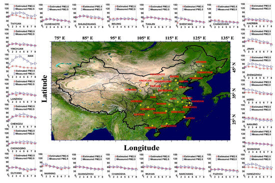
Figure 5.
Annual average hourly PM2.5 concentrations of 26 typical cities in 2017.
4.3. Model Performance in Typical Cases
The analysis in this section shows that the model is sensitive to the estimates of the ground-level hourly PM2.5 concentrations. The model performance was tested for typical cases such as haze events and dust events.
4.3.1. Model Performance during Haze Events
A serious haze event occurred in South China on December 24, 2017. Based on the temporal, geographical, and underlying surface-weighted regression models, the PM2.5 concentrations for 8 h on December 24, 2017 were estimated. The results are shown in Figure 6. The PM2.5 estimation results were highly consistent with the monitoring data. The results show that haze occurred in Jiangxi, Hunan, Hubei, Anhui, Zhejiang, and Shanghai and that the PM2.5 concentration exceeded 100 µg/m3. The PM2.5 concentration was relatively high in the morning and then decreased gradually. The geostationary satellite retrieval results were also used to monitor the haze dissipation process. The PM2.5 concentration began to decrease at 2:00 UTC in Anhui Province. Next, the haze in Zhejiang Province also began to dissipate. Although haze was still present in Jiangxi, Hunan, and Hubei provinces, the PM2.5 concentration decreased. Until 7:00 UTC, the PM2.5 concentration over the middle and lower reaches of the Yangtze River was below 70 µg/m3. In the middle and lower reaches of the Yangtze River on the 24th, the PM2.5 concentration varied by more than 100 µg/m3 in 8 h. The geostationary satellite satisfied the requirements for continuous, real-time, and large-scale monitoring of PM2.5 under these extreme weather conditions.
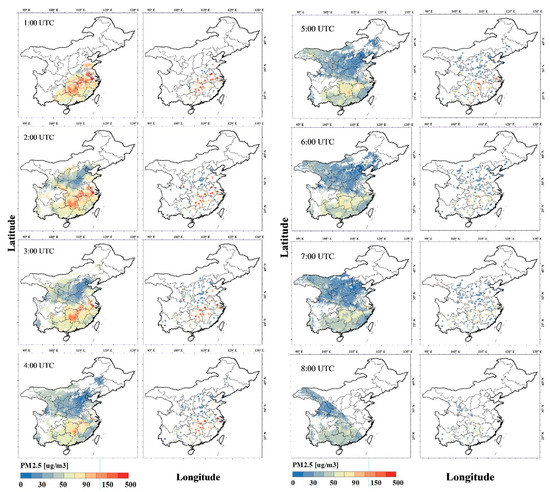
Figure 6.
Predicted and observed PM2.5 concentrations in study area during a haze event on December 24, 2017. Columns 1 and 3 are the model estimation results, and columns 2 and 4 are the site observation data (the column number is 1, 2, 3, 4 from left to right).
4.3.2. Model Performance during Dust Events
Dust storms are another weather event in which the PM2.5 concentrations rise rapidly. An early warning and monitoring system for dust storms is particularly important. During severe dust storms, ground monitoring of PM2.5 is often inaccurate owing to excessive wind speed and shows an abrupt increase in particulate matter concentration. This problem makes accurate monitoring of PM2.5 concentrations difficult. However, geostationary satellites provide stable and continuous monitoring platforms that are not affected by extreme weather near the ground. The model’s performance during dust events was also tested. Figure 7 shows a dust plume with a high PM2.5 concentration that spreads from northwestern to northeastern China in May 2017. Dust was widespread in the north-central part of China. The PM2.5 concentrations in Inner Mongolia, Southwestern Gansu, Ningxia, Northern Shaanxi, Shanxi, and Hebei provinces were more than 200 µg/m3. The geostationary satellite successfully captured the movement of the dust plume (Figure 7), which gradually moved from Inner Mongolia Province to Northeast China. The PM2.5 concentration in western Inner Mongolia began to decrease gradually. After 6:00 UTC, the dust in western Inner Mongolia, southeastern Gansu, and Ningxia provinces began to weaken gradually. Until 8:00 UTC, the PM2.5 concentration in the dust plume decreased to approximately 70 µg/m3. The effective ground-based PM2.5 observation data were limited on May 4 and were concentrated mainly in the North China Plain. There were no ground monitoring data for Inner Mongolia, which was seriously affected by dust. The satellite-based PM2.5 concentration estimation results are still highly consistent with the observation data.
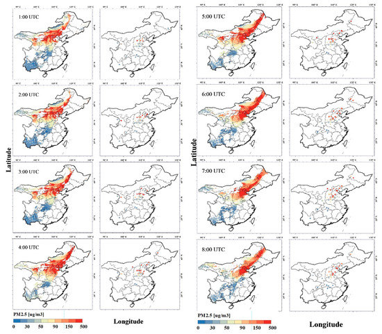
Figure 7.
Predicted PM2.5 concentrations in study area during a dust event on May 4, 2017. Columns 1 and 3 are the model estimation results, and columns 2 and 4 are the site observation data (the column number is 1, 2, 3, and 4 from left to right).
5. Discussion
The AHI AOD was calculated by a novel algorithm that uses a non-Lambertian forward model coupled with a surface bidirectional reflectance distribution function model. The accuracy of the retrieved AHI AOD is comparable to that of the MODIS AOD (C6). The coverage rate of the AHI AOD is better than that of the Japan Meteorological Agency (JMA)/AOD products [9].
Unlike the models used in previous studies, the IGTWR model generalized the geographical distance. Hu et al. [24] used the spatial distance as the weight parameter; later, Huang et al. [29] generalized this distance to a geographical and temporal distance by introducing the day number into the model. In this study, we also use the day, hour, and land use type to construct the distance. The R2 value of the observed and predicted hourly PM2.5 in our GTLWR fitting set is 0.886, and the RMSE is 12.18 µg/m3 for the 437,642 samples. In addition, the R2 value of the observed and predicted daily PM2.5 concentrations obtained by IGTWR is 0.87, and the RMSE is 14.56 µg/m3 for 60,810 samples in China. The IGTWR model still outperforms the GTWR model with a sample set that was approximately eight times larger.
In this study, ground-level hourly PM2.5 concentrations in central and eastern China with high estimation accuracy were obtained. This achievement is meaningful for high-temporal-resolution air quality monitoring in China. Although the relevant research has been reported, which mainly focus on a relatively small region. Wang et al. [20] estimated the hourly PM2.5 concentrations based on an improved linear mixed effects model for the Beijing–Tianjin–Hebei region with Himawari-8 data. The RMSE of the tenfold cross-validation result for the Beijing–Tianjin–Hebei region in that study was 24.3 µg/m3 for 83,989 samples, whereas, in this study, we obtained the PM2.5 validation result for central and eastern China with an RMSE of 12.18 µg/m3 for 437,642 samples.
The general spatial pattern of the hourly PM2.5 pollution in China obtained by IGTWR is similar to that in previous studies [10,25], except that GTLWR shows that the Fenwei Plain becomes a PM2.5 hotspot, and the North China Plain has lower PM2.5 concentrations. The temporal characteristics of the satellite-based hourly PM2.5 data in central and eastern China are also revealed. PM2.5 showed an intraday decreasing trend, and the different performance in the eastern and western parts of our study area may be related to the timing of solar radiation [31].
The performance of the IGTWR model in extreme weather conditions, especially during dust events, is similar to the dust detection results reported in a previous study. She et al. [6] introduced an enhanced dust intensity index based on Himawari-8 brightness temperature data. The distribution of the hourly PM2.5 concentration estimated by IGTWR on May 4, 2017 is consistent with the dust intensity index.
6. Conclusions
A temporally, geographically, and underlying surface weighted-regression model of the hourly PM2.5 concentration was applied to central and eastern China in 2017. In this study, the weight of the generalized geographically weighted model was constructed using the longitude, latitude, day, hour, and land use type, and the AHI AOD, surface relative humidity, and boundary layer height data were used as independent variables. The hourly PM2.5 concentrations in eastern and central China were estimated at eight times (1:00, 2:00, 3:00, 4:00, 5:00, 6:00, 7:00, and 8:00 UTC) in 2017.
The model fitting and cross-validation performance are satisfactory. For the modelling set, the R2 value of the measured and predicted PM2.5 is 0.886, and the RMSE is only 12.180 µg/m3. The tenfold cross-validation results of the regression model are also acceptable; the correlation coefficient R2 of the measured and predicted PM2.5 is 0.784, and the RMSE is 20.104 µg/m3, which is only 8 µg/m3 higher than that of the modelling set. The validation results showed highly predictable and reliable PM2.5 estimation.
There are significant regional pollution characteristics over central and eastern China in 2017. Fine particulate matter pollution events are concentrated mainly in the North China Plain, Guanzhong Plain, Fenwei Plain, middle and lower reaches of the Yangtze River, South China, and Sichuan Basin. The ground-level PM2.5 concentration is negatively correlated with the solar radiation. The predicted and measured values of the PM2.5 concentration are highly consistent throughout the study area. The model results represent the actual distribution characteristics of PM2.5 in central and eastern China.
The model designed in this study can monitor the occurrence, development, and termination of extreme weather events. The predicted PM2.5 concentration is very similar to the observed PM2.5 concentration. Satellite-based hourly PM2.5 monitoring will play an important role in predicting extreme weather events and providing warnings in advance.
Author Contributions
Conceptualization, Y.X. and Y.L.; methodology, Y.L. and Y.X.; software, Y.C.; validation, J.G., Y.W. and Y.C.; formal analysis, Y.L. and L.S.; investigation, K.Q. and C.F.; resources, C.F. and Y.W.; data curation, A.T.; writing—Original draft preparation, Y.L.; writing—Review and editing, Y.X. and A.T.; visualization, Z.W.; supervision, Y.X.; project administration, J.G.; funding acquisition, Y.X. All authors have read and agreed to the published version of the manuscript.
Funding
This work was supported by the Ministry of Science and Technology (MOST) of China under grant no. 2016YFC02005 and the National Natural Science Foundation of China (NSFC) under grant nos. 41471260, 41471306 and 41590853.
Acknowledgments
This work was supported by the Ministry of Science and Technology (MOST) of China under grant no. 2016YFC02005 and the National Natural Science Foundation of China (NSFC) under grant nos. 41471260, 41471306 and 41590853. The data for analysis were obtained from JMA, ECMWF, the National Real-time Air Quality Publishing Platform, and the Resource and Environment Data Cloud Platform. We thank the investigators and their staffs for establishing and maintaining the important data used in this investigation.
Conflicts of Interest
The authors declare no conflict of interest.
References
- Kloog, I.; Nordio, F.; Coull, B.A.; Schwartz, J. Incorporating local land use regression and satellite aerosol optical depth in a hybrid model of spatiotemporal PM2.5 exposures in the mid-atlantic states. Environ. Sci. Technol. 2012, 6, 11913–11921. [Google Scholar] [CrossRef] [PubMed]
- Husar, R.B. Characterization of tropospheric aerosols over the oceans with the NOAA advanced very high resolution radiometer optical thickness operational product. J. Geophys. Res. 1997, 102, 16889–16909. [Google Scholar] [CrossRef]
- Kahn, R.; Banerjee, P.; McDonald, D. Sensitivity of multiangle imaging to natural mixtures of aerosols over ocean. J. Geophys. Res. Atmos. 2001, 106, 18219–18238. [Google Scholar] [CrossRef]
- Levy, R.C.; Remer, L.A.; Mattoo, S.; Vermote, E.F.; Kaufman, Y.J. Second-generation operational algorithm: Retrieval of aerosol properties over land from inversion of Moderate Resolution Imaging Spectroradiometer spectral reflectance. J. Geophys. Res. Atmos. 2007, 112. [Google Scholar] [CrossRef]
- McGill, M.J.; Vaughan, M.A.; Trepte, C.R.; Hart, W.D.; Hlavka, D.L.; Winker, D.M.; Kuehn, R. Airborne validation of spatial properties measured by the CALIPSO lidar. J. Geophys. Res. Atmos. 2007, 112. [Google Scholar] [CrossRef]
- She, L.; Xue, Y.; Yang, X.; Guang, J.; Li, Y.; Che, Y.; Fan, C.; Xie, Y. Dust detection and intensity estimation using himawari-8/AHI observation. Remote Sens. 2018, 10, 490. [Google Scholar] [CrossRef]
- Zhang, W.; Xu, H.; Zheng, F. Aerosol optical depth retrieval over East Asia using himawari-8/AHI data. Remote Sens. 2018, 10, 137. [Google Scholar] [CrossRef]
- Zhang, Z.; Fan, M.; Wu, W.; Wang, Z.; Tao, M.; Wei, J.; Wang, Q. A simplified aerosol retrieval algorithm for Himawari-8 advanced himawari imager over Beijing. Atmos. Environ. 2019, 199, 127–135. [Google Scholar] [CrossRef]
- She, L.; Xue, Y.; Yang, X.; Leys, J.; Guang, J.; Che, Y.; Fan, C.; Xie, Y.; Li, Y. Joint retrieval of aerosol optical depth and surface reflectance over land using geostationary satellite data. IEEE Trans. Geosci. Remote Sens. 2019, 57, 1489–1501. [Google Scholar] [CrossRef]
- He, Q.; Huang, B. Satellite-based mapping of daily high-resolution ground PM2.5 in China via space-time regression modeling. Remote Sens. Environ. 2018, 206, 72–83. [Google Scholar] [CrossRef]
- Koelemeijer, R.B.A.; Homan, C.D.; Matthijsen, J. Comparison of spatial and temporal variations of aerosol optical thickness and particulate matter over Europe. Atmos. Environ. 2006, 40, 5304–5315. [Google Scholar] [CrossRef]
- Lin, C.; Li, Y.; Lau, A.K.H.; Deng, X.; Tse, T.K.T.; Fung, J.C.H.; Li, C.; Li, Z.; Lu, X.; Zhang, X.; et al. Estimation of long-term population exposure to PM2.5 for dense urban areas using 1-km MODIS data. Remote Sens. Environ. 2016, 179, 13–22. [Google Scholar] [CrossRef]
- Zhang, Y.; Li, Z. Remote sensing of atmospheric fine particulate matter (PM2.5) mass concentration near the ground from satellite observation. Remote Sens. Environ. 2015, 160, 252–262. [Google Scholar] [CrossRef]
- Gupta, P.; Christopher, S.A. Seven year particulate matter air quality assessment from surface and satellite measurements. Atmos. Chem. Phys. (ACP) Discuss. (ACPD) 2008, 8, 3311–3324. [Google Scholar] [CrossRef]
- Meng, X.; Fu, Q.; Ma, Z.; Chen, L.; Zou, B.; Zhang, Y.; Xue, W.; Wang, J.; Wang, D.; Kan, H.; et al. Estimating ground-level PM10 in a Chinese city by combining satellite data, meteorological information and a land use regression model. Environ. Pollut. 2016, 208, 177–184. [Google Scholar] [CrossRef]
- Lee, H.J.; Liu, Y.; Coull, B.A.; Schwartz, J.; Koutrakis, P. A novel calibration approach of MODIS AOD data to predict PM2.5 concentrations. Atmos. Chem. Phys. (ACP) Discuss. (ACPD) 2011, 11, 9769–9795. [Google Scholar] [CrossRef]
- Liu, Y.; Sarnat, J.A.; Kilaru, V.; Jacob, D.J.; Koutrakis, P. Estimating ground-level PM2.5 in the Eastern United States using satellite remote sensing. Environ. Sci. Technol. 2005, 39, 3269–3278. [Google Scholar] [CrossRef]
- van Donkelaar, A.; Martin, R.V.; Spurr, R.J.; Burnett, R.T. High-resolution satellite-derived PM2.5 from optimal estimation and geographically weighted regression over North America. Environ. Sci. Technol. 2015, 49, 10482–10491. [Google Scholar] [CrossRef]
- You, W.; Zang, Z.; Zhang, L.; Zhang, M.; Pan, X.; Li, Y. A nonlinear model for estimating ground-level PM10 concentration in Xi’an using MODIS aerosol optical depth retrieval. Atmos. Res. 2016, 168, 169–179. [Google Scholar] [CrossRef]
- Wang, W.; Mao, F.; Du, L.; Pan, Z.; Gong, W.; Fang, S. Deriving Hourly PM2.5 Concentrations from Himawari-8 AODs over Beijing–Tianjin–Hebei in China. Remote Sens. 2017, 9, 858. [Google Scholar] [CrossRef]
- Zeng, Q.; Chen, L.; Zhu, H.; Wang, Z.; Wang, X.; Zhang, L.; Gu, T.; Zhu, G.; Zhang, Y. Satellite-based estimation of hourly PM2.5 concentrations using a vertical-humidity correction method from Himawari-AOD in Hebei. Sensors 2018, 18, 3456. [Google Scholar] [CrossRef] [PubMed]
- Chen, J.; Yin, J.; Zang, L.; Zhang, T.; Zhao, M. Stacking machine learning model for estimating hourly PM2.5 in China based on Himawari 8 aerosol optical depth data. Sci. Total Environ. 2019, 697, 134021. [Google Scholar] [CrossRef] [PubMed]
- Liu, J.; Weng, F.; Li, Z.; Cribb, C.M. Hourly PM2.5 estimates from a geostationary satellite based on an ensemble learning algorithm and their spatiotemporal patterns over central east China. Remote Sens. 2019, 11, 2120. [Google Scholar] [CrossRef]
- Hu, X.; Waller, L.A.; Al-Hamdan, M.Z.; Crosson, W.L.; Estes, M.G.; Estes, S.M.; Quattrochi, D.A.; Sarnat, J.A.; Liu, Y. Estimating ground-level PM2.5 concentrations in the southeastern U.S. using geographically weighted regression. Environ. Res. 2013, 121, 1–10. [Google Scholar] [CrossRef] [PubMed]
- Ma, Z.; Hu, X.; Huang, L.; Bi, J.; Liu, Y. Estimating ground-level PM2.5 in China using satellite remote sensing. Environ. Sci. Technol. 2014, 48, 7436–7444. [Google Scholar] [CrossRef] [PubMed]
- He, Q.; Geng, F.; Li, C.; Yang, S.; Wang, Y.; Mu, H.; Zhou, G.; Liu, X.; Gao, W.; Cheng, T.; et al. Long-term characteristics of satellite-based PM2.5 over East China. Sci. Total Environ. 2018, 612, 1417–1423. [Google Scholar] [CrossRef]
- Xu, X.; Liu, J.; Zhuang, D. Remote sensing Monitoring methods of land use/cover changes in national scale. J. Anhui Agric. Sci. 2012, 40, 2365–2369. (In Chinese) [Google Scholar]
- Miao, Y.; Liu, S.; Guo, J.; Huang, S.; Yan, Y.; Lou, M. Unraveling the relationships between boundary layer height and PM2.5 pollution in China based on four-year radiosonde measurements. Environ. Pollut. 2018, 243, 1186–1195. [Google Scholar] [CrossRef]
- Huang, B.; Wu, B.; Barry, M. Geographically and temporally weighted regression for modeling spatio-temporal variation in house prices. Int. J. Geogr. Inf. Sci. 2010, 24, 383–401. [Google Scholar] [CrossRef]
- Hastie, T.; Tibshirani, R. Generalized Additive Models; John Wiley & Sons, Inc.: Hoboken, NJ, USA, 1990. [Google Scholar]
- Guo, Y.; Hong, S.; Feng, N.; Zhuang, Y.; Zhang, L. Spatial distributions and temporal variations of atmospheric aerosols and the affecting factors: A case study for a region in Central China. Int. J. Remote Sens. 2012, 33, 3672–3692. [Google Scholar] [CrossRef]
- Guo, J.; Miao, Y.; Zhang, Y.; Liu, H.; Li, Z.; Zhang, W.; He, J.; Lou, M.; Yan, Y.; Bian, L.; et al. The climatology of planetary boundary layer height in China derived from radiosonde and reanalysis data. Atmos. Chem. Phys. 2016, 16, 13309–13319. [Google Scholar] [CrossRef]
- Wang, L.; Gong, W.; Xia, X.; Zhu, J.; Li, J.; Zhu, Z. Long-term observations of aerosol optical properties at Wuhan, an urban site in Central China. Atmos. Environ. 2015, 101, 94–102. [Google Scholar] [CrossRef]


© 2020 by the authors. Licensee MDPI, Basel, Switzerland. This article is an open access article distributed under the terms and conditions of the Creative Commons Attribution (CC BY) license (http://creativecommons.org/licenses/by/4.0/).