Triple-Pair Constellation Configurations for Temporal Gravity Field Retrieval


Abstract
:
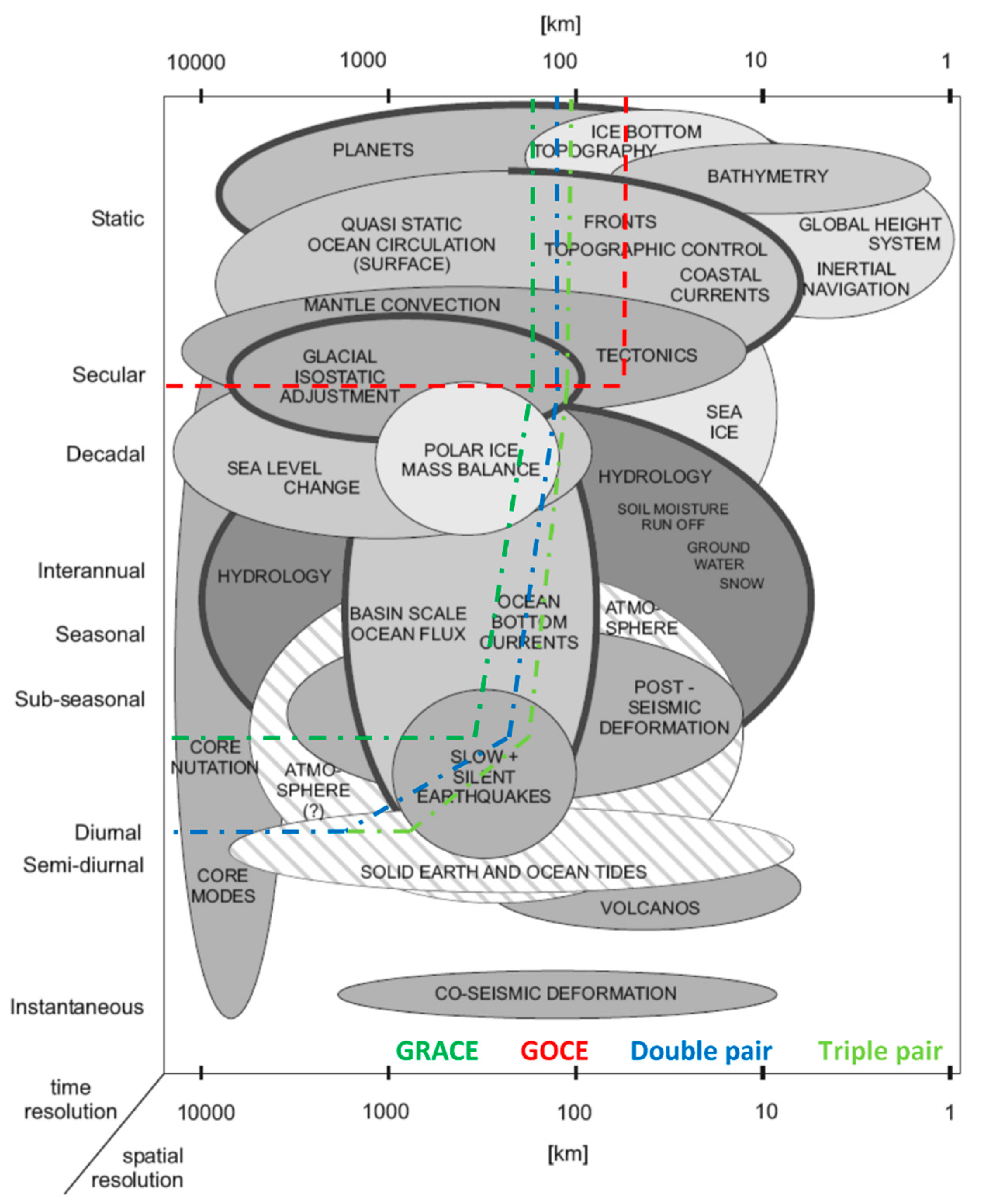
1. Introduction
2. Constellation Design
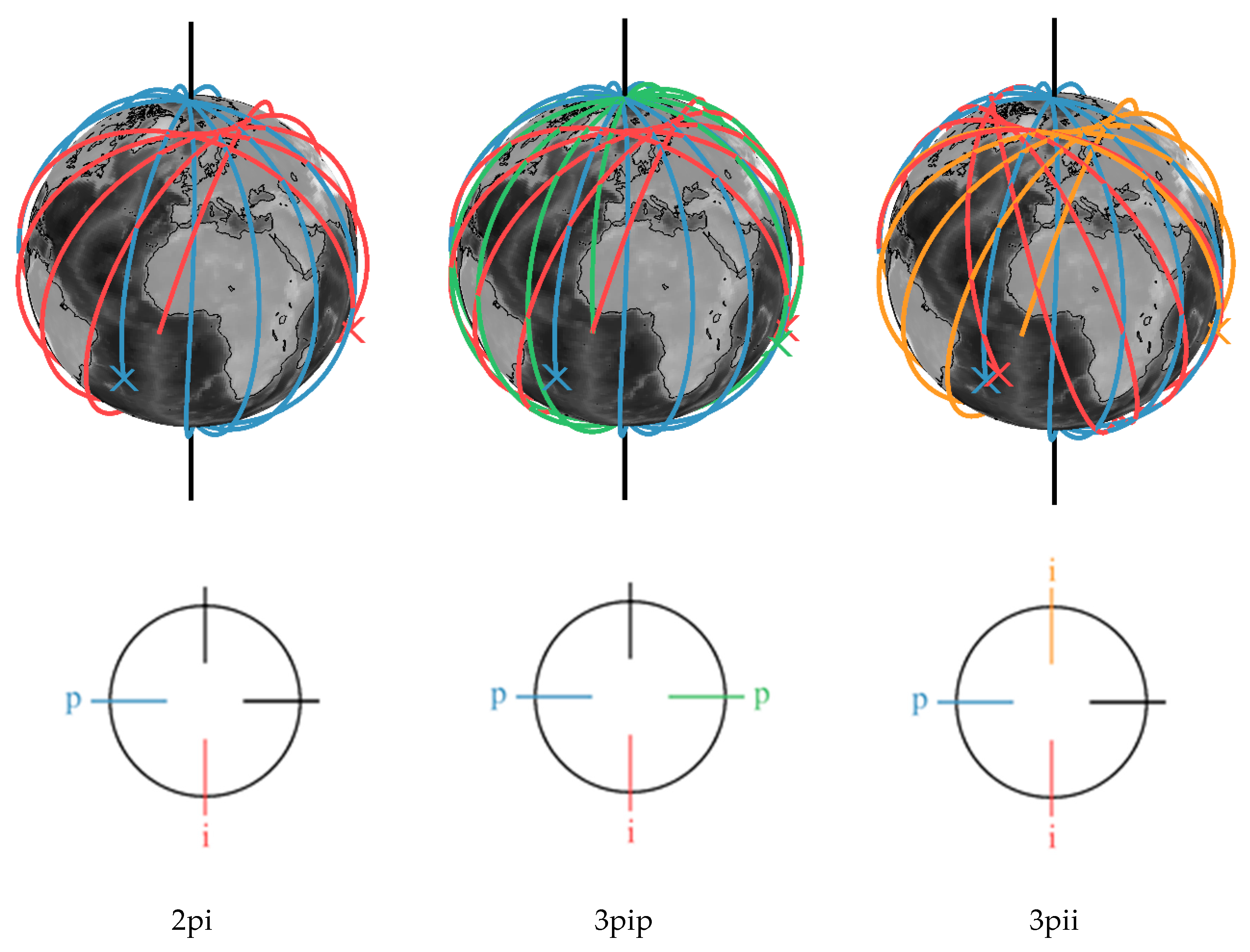
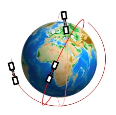
2.1. Orbit Constellation
2.2. Space-Time Sampling
3. Closed-Loop Simulation
3.1. Numerical Simulator
3.2. Noise
3.2.1. GRACE-Like Noise
3.2.2. NGGM Noise
4. Results
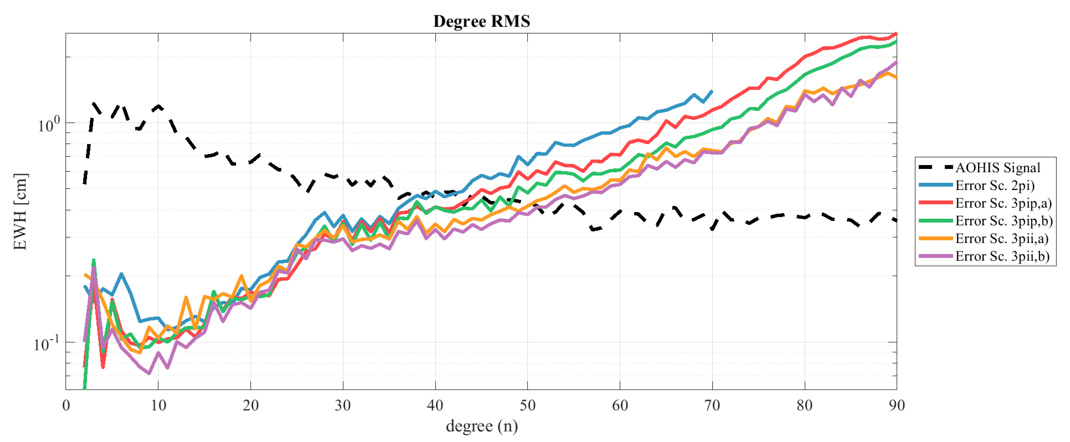
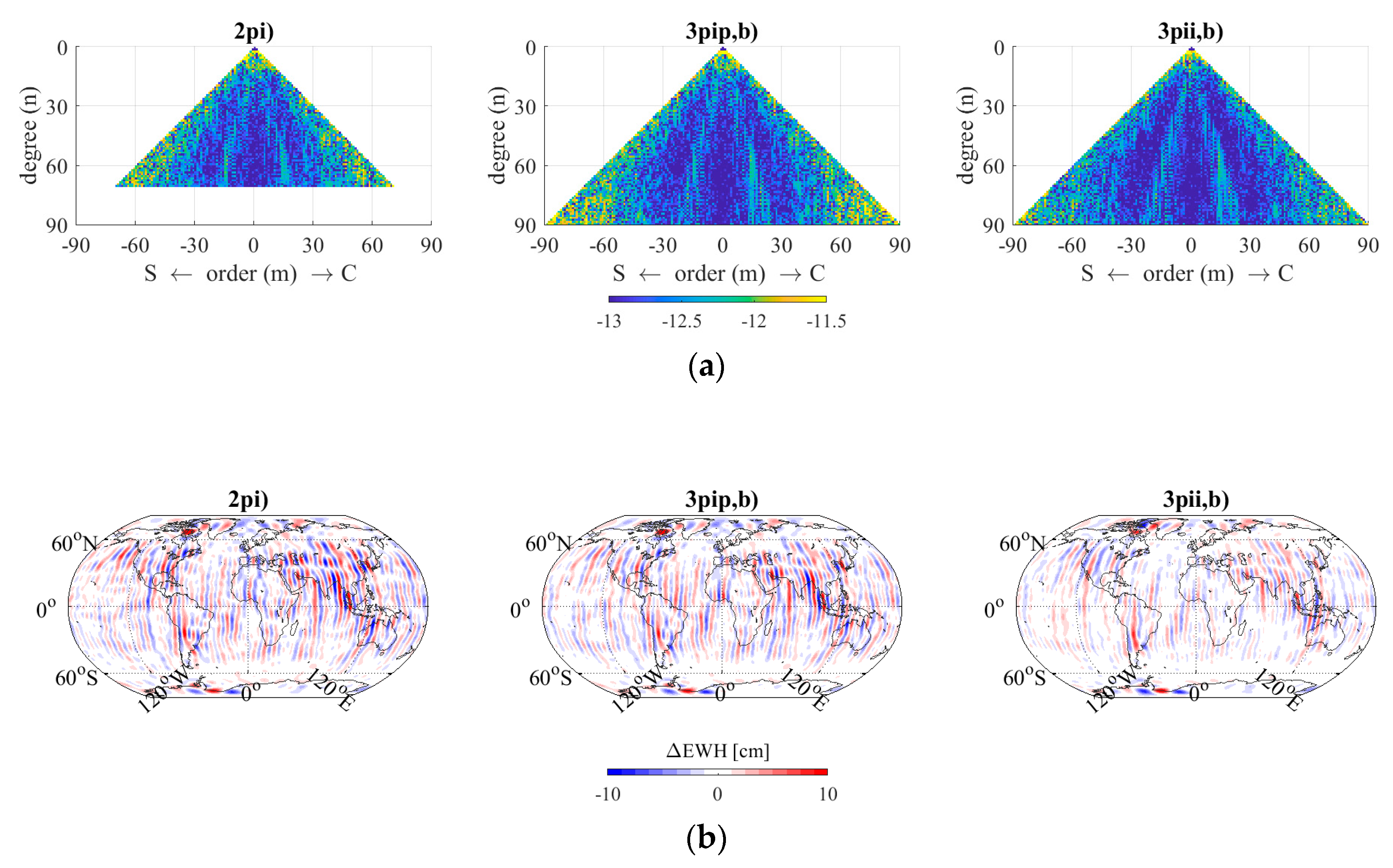
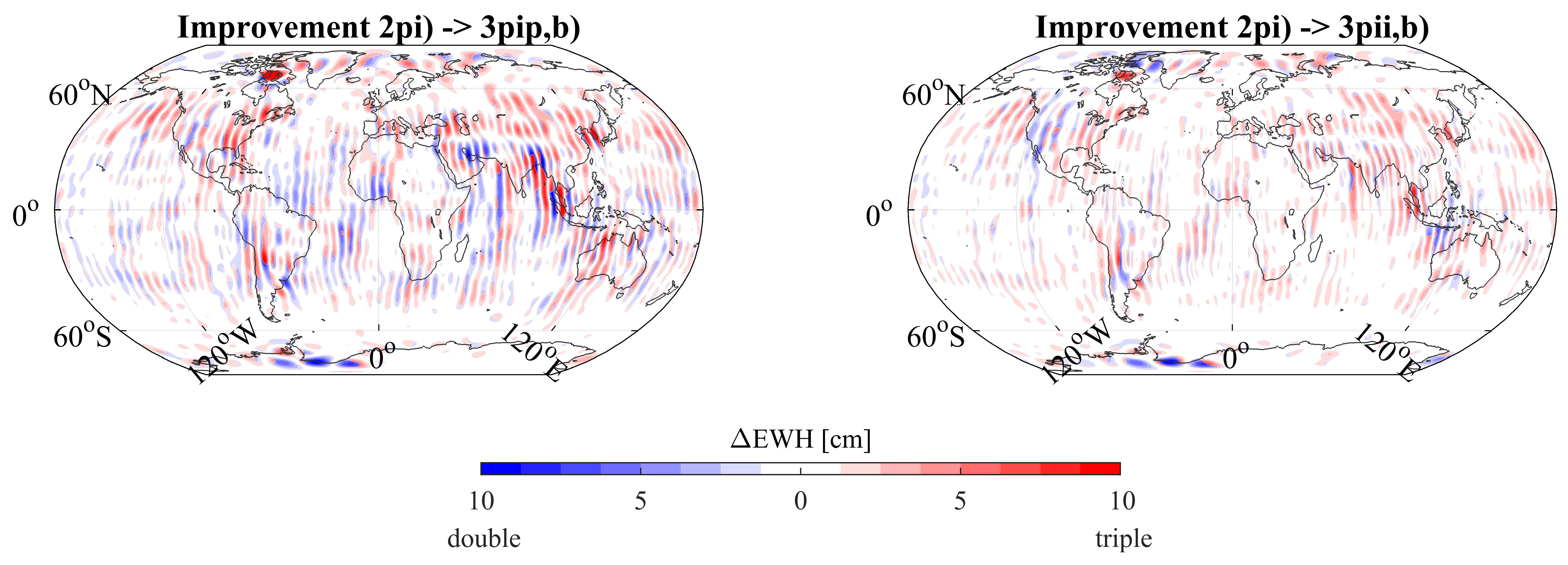
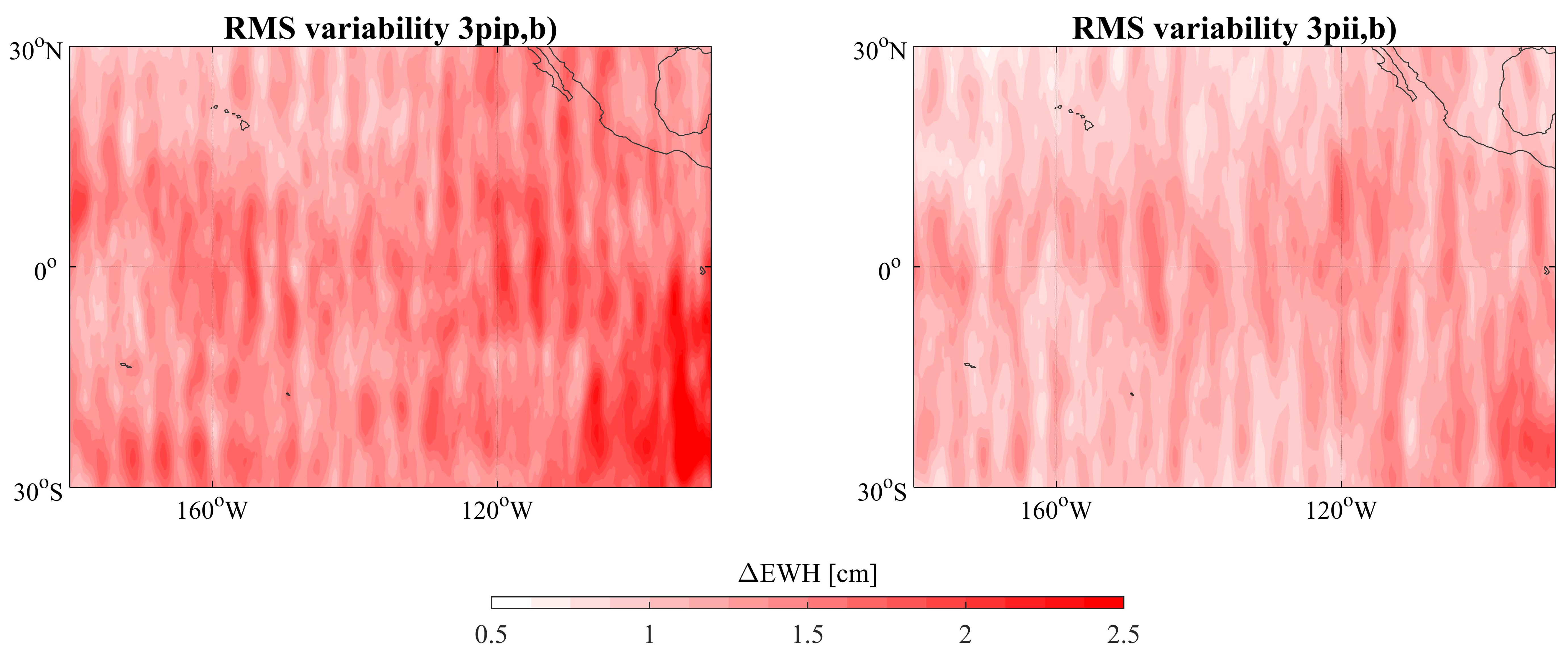
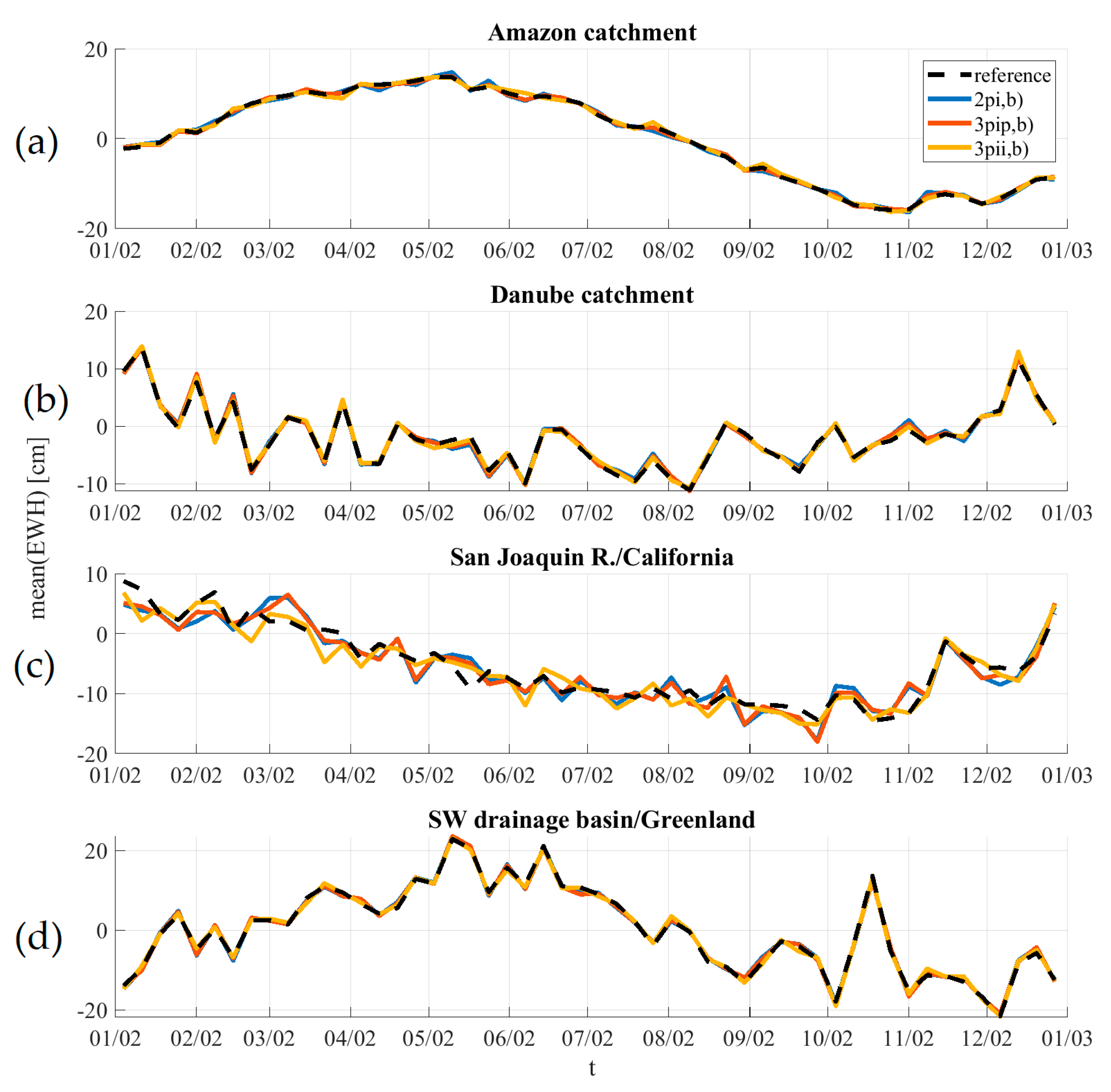
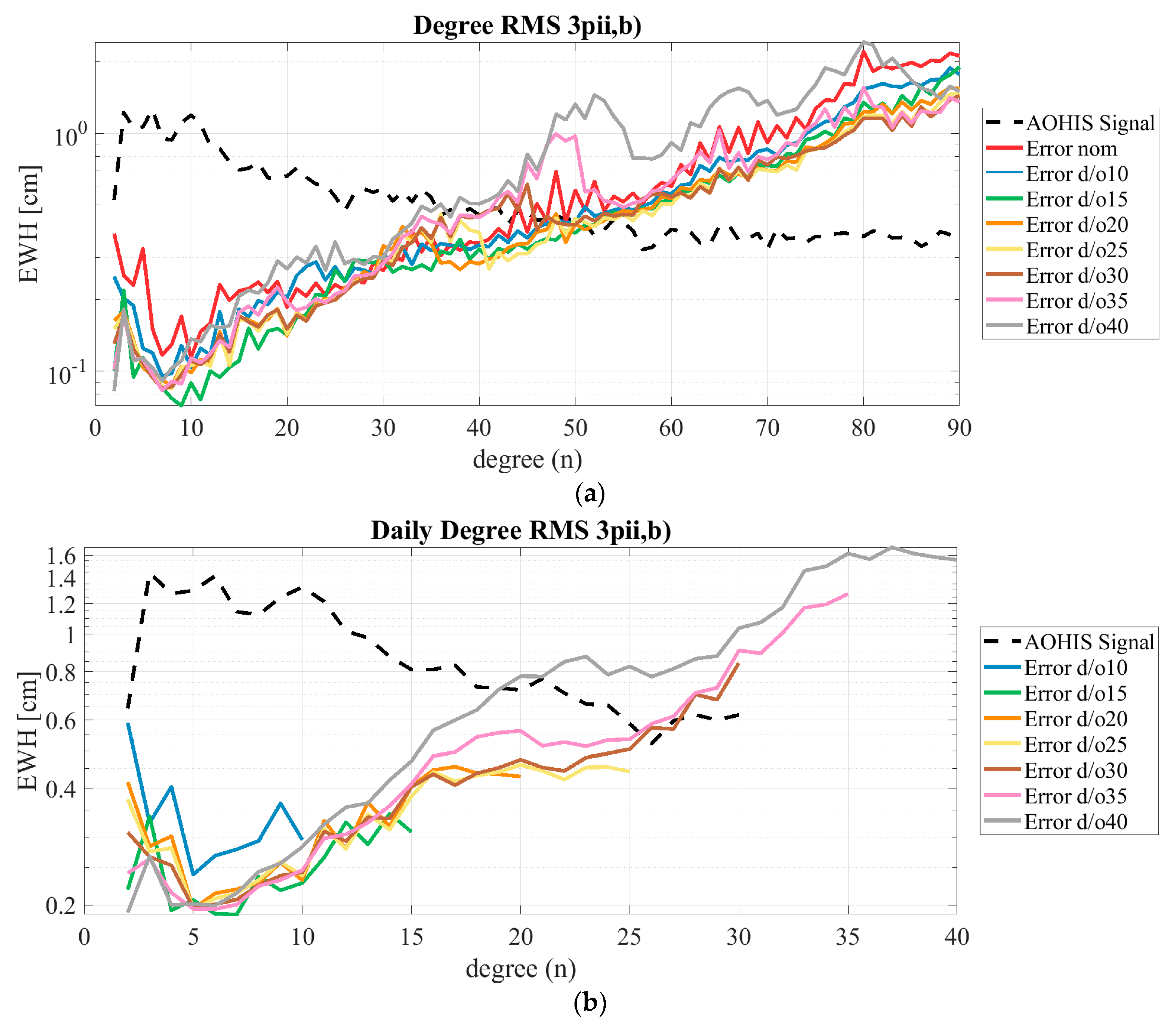
4.1. Double vs. Triple Pairs
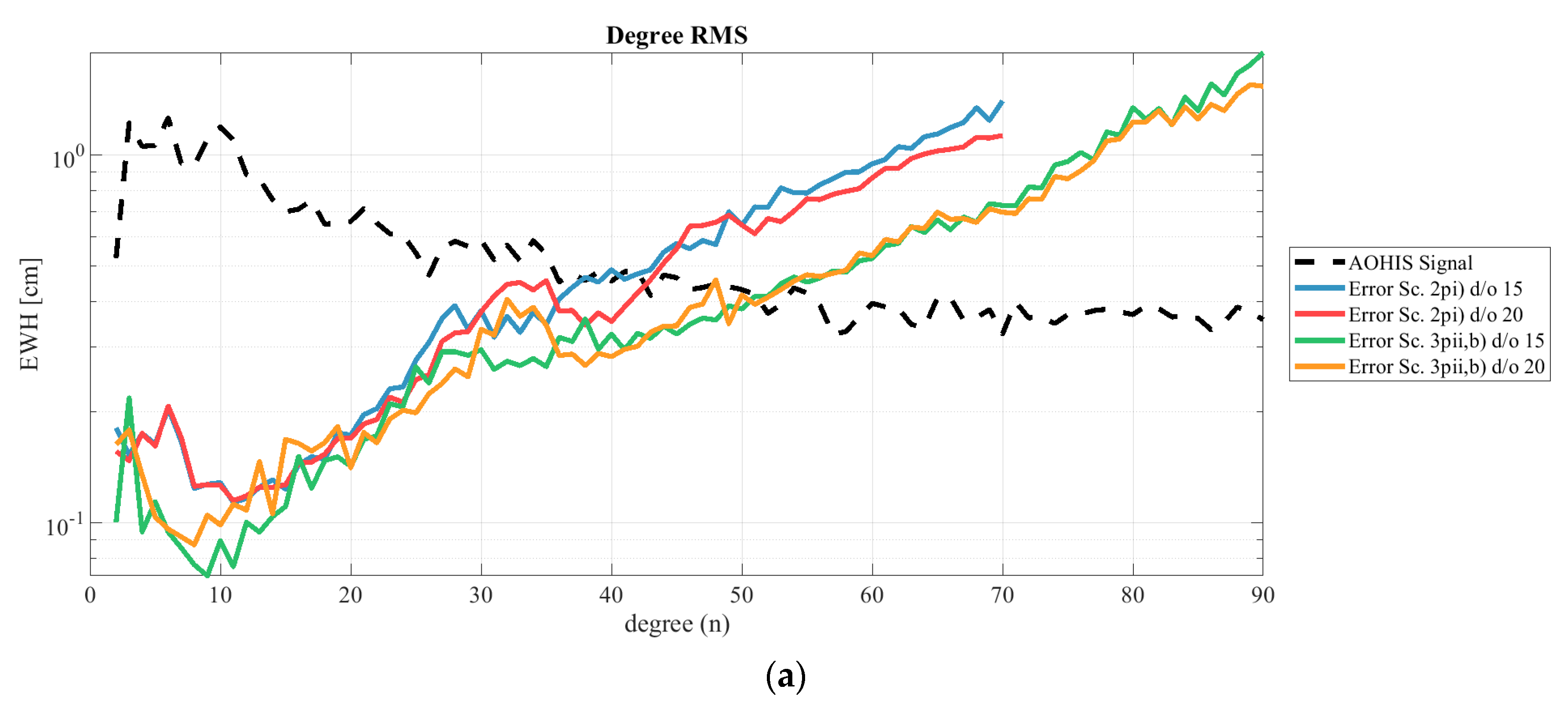
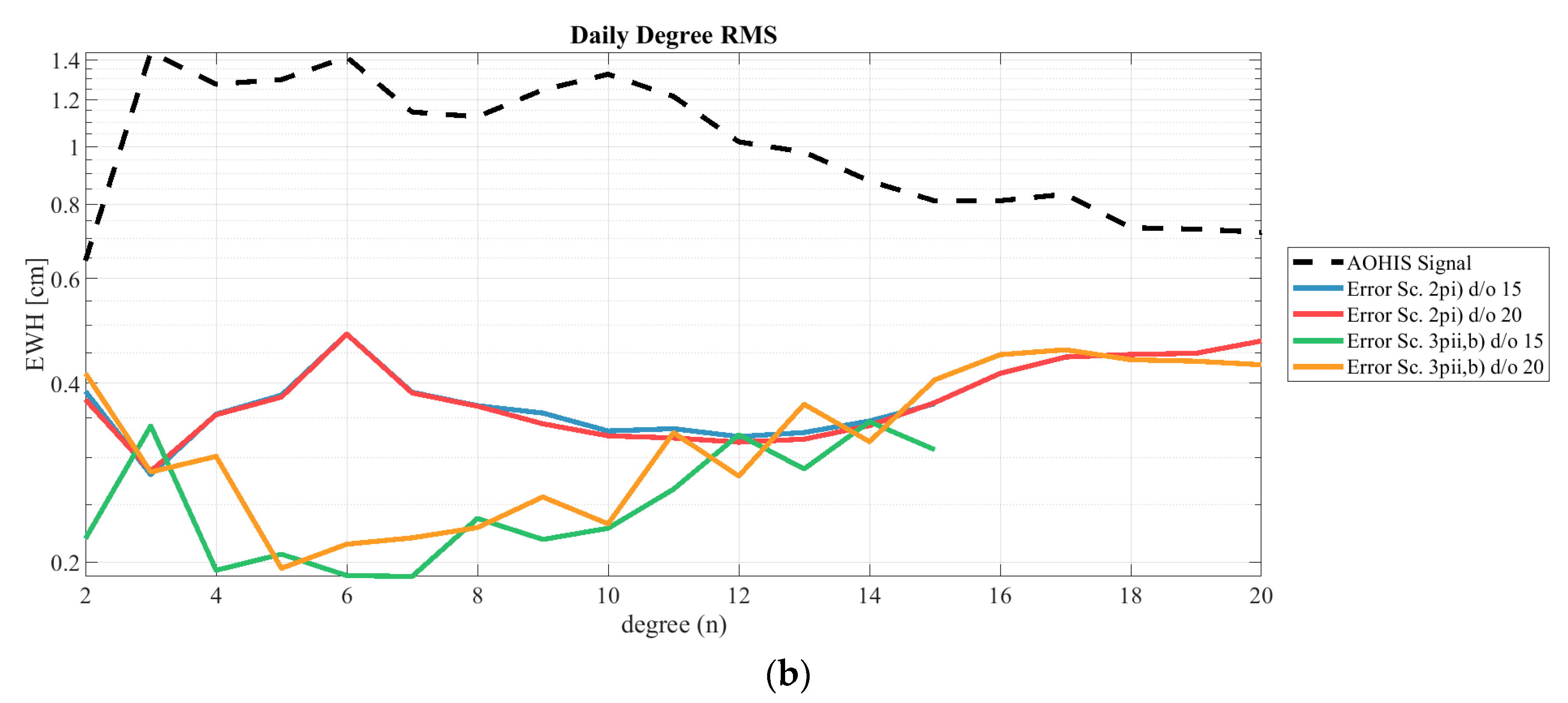
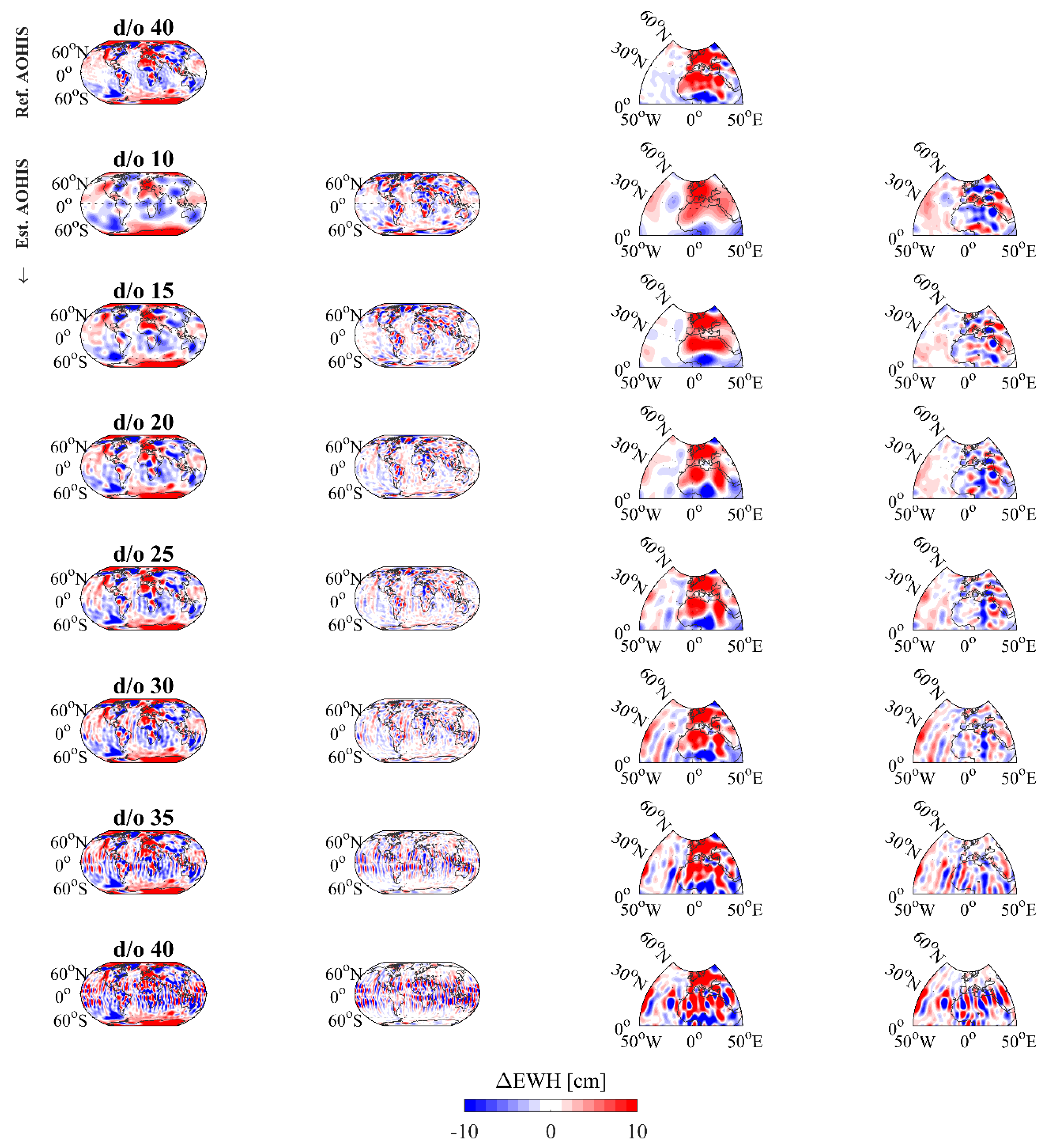
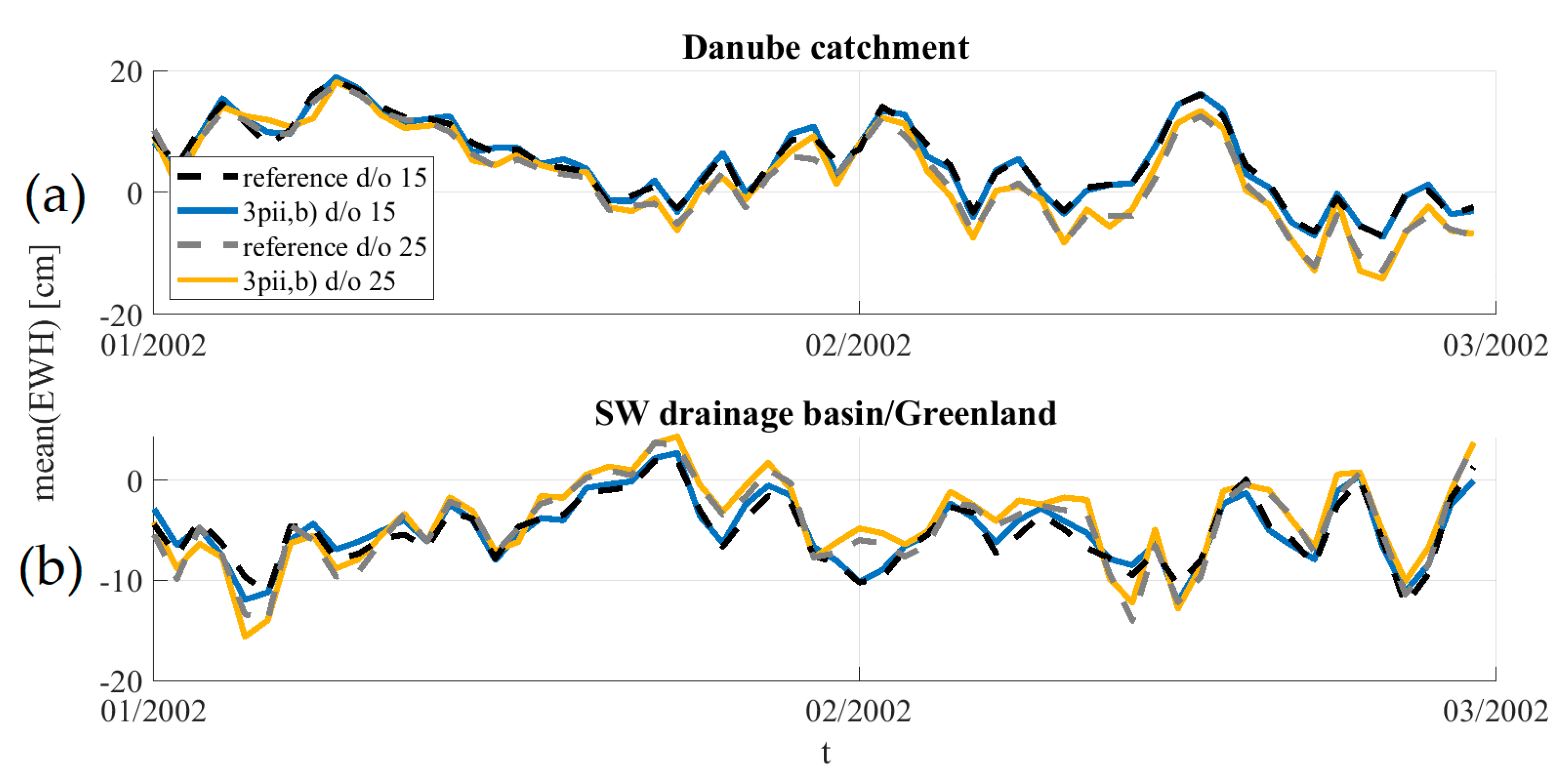
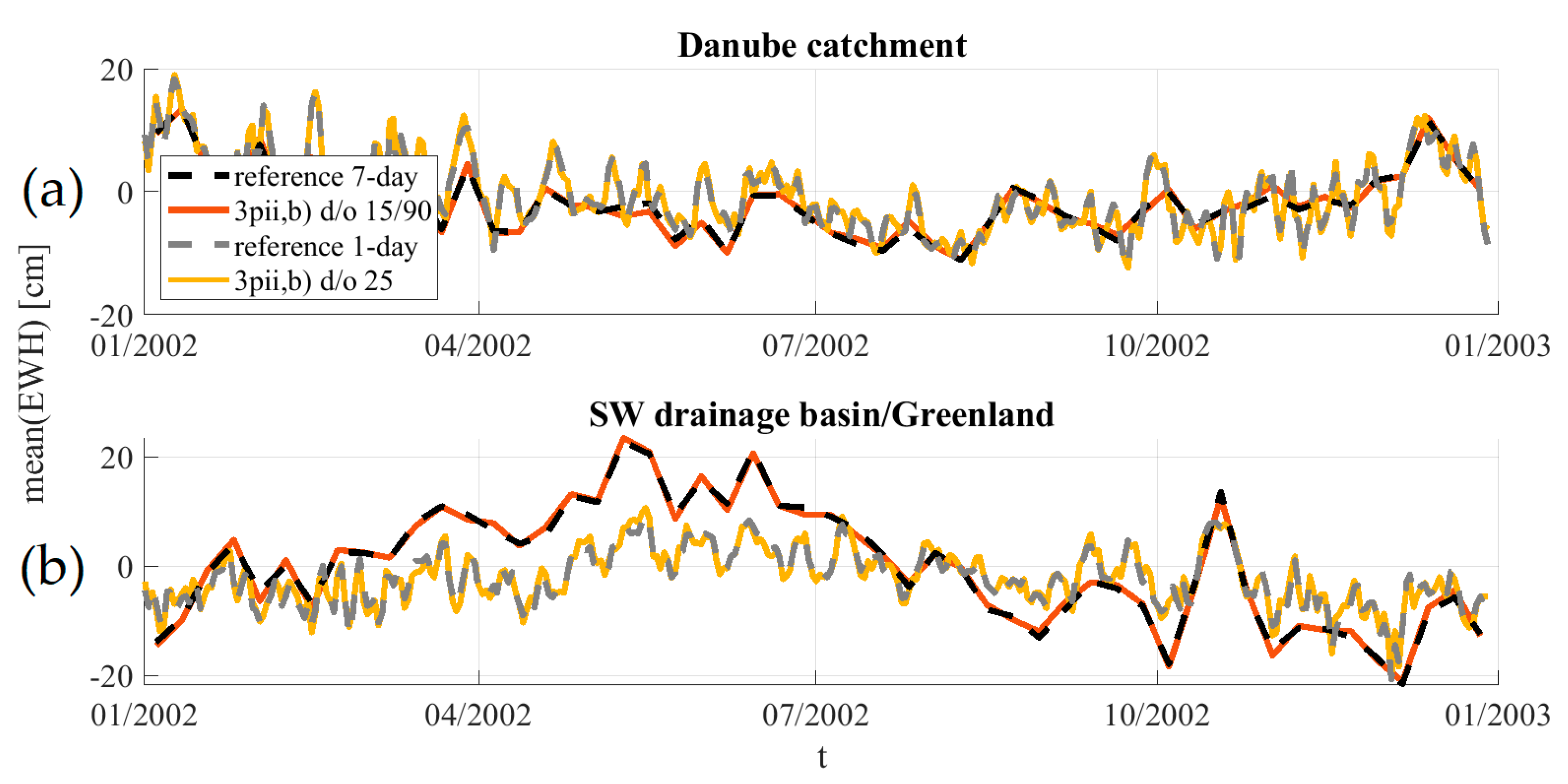
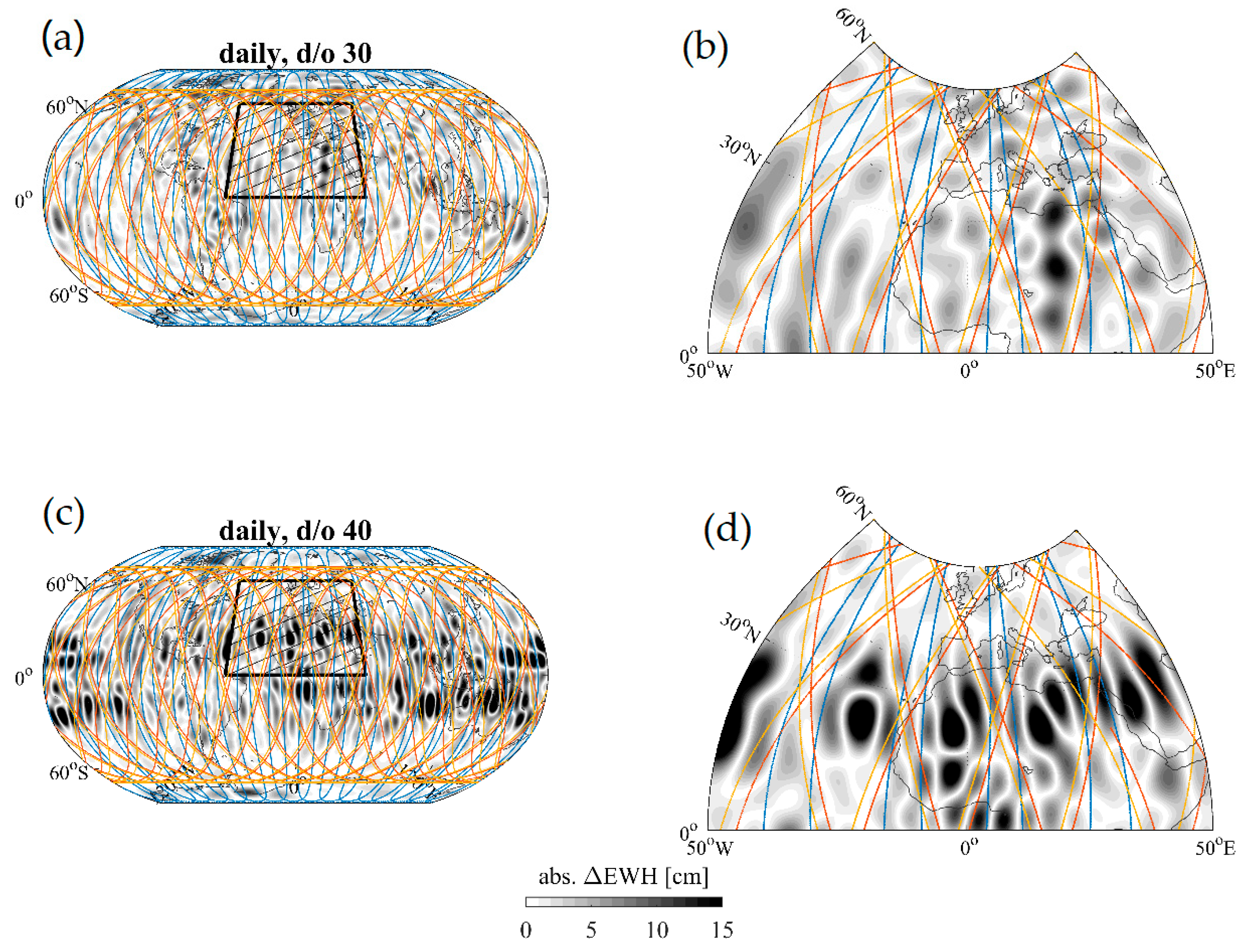
4.2. Higher-Degree Daily Resolution
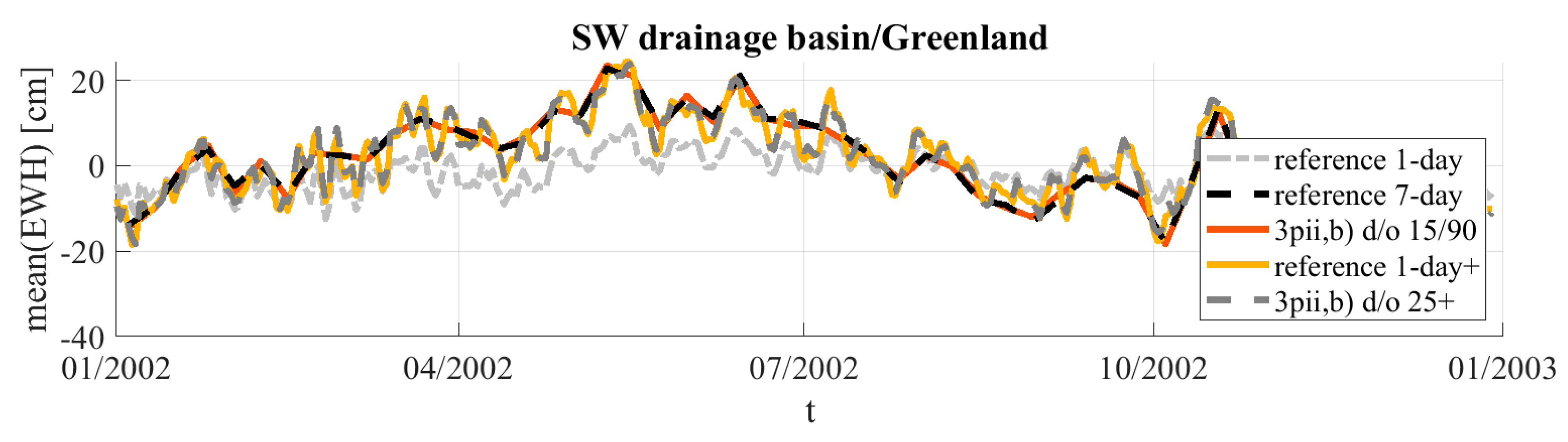
4.3. Applications
5. Conclusions
Author Contributions
Funding
Acknowledgments
Conflicts of Interest
References
- Reigber, C.; Schwintzer, P.; Lühr, H. The CHAMP geopotential mission, Bollettino di Geofisica Teoretica ed Applicata, 40/ 3-4, September-December 1999. In Proceedings of the Second Joint Meeting of the International Gravity and the International Geoid Commission, Trieste, Italy, 7–12 September 1998; Marson, I., Sünkel, H., Eds.; 1999; pp. 285–6729, ISSN 0006-6729. [Google Scholar]
- Tapley, B.D.; Bettadpur, S.; Watkins, M.; Reigber, C. The gravity recovery and climate experiment experiment, mission overview and early results. Geophys. Res. Lett. 2004, 31, L09607. [Google Scholar] [CrossRef] [Green Version]
- Kornfeld, R.P.; Arnold, B.W.; Gross, M.A.; Dahya, N.T.; Klipstein, W.M.; Gath, P.F.; Bettadpur, S. GRACE-FO: The Gravity Recovery and Climate Experiment Follow-On Mission. J. Spacecr. Rocket. 2019, 56, 931–951. [Google Scholar] [CrossRef]
- Rodell, M.; Famiglietti, J.S.; Wiese, D.N.; Reager, J.T.; Beaudoing, H.K.; Landerer, F.W.; Lo, M.H. Emerging trends in global freshwater availability. Nature 2018, 557, 651–659. [Google Scholar] [CrossRef]
- Forootan, E.; Didova, O.; Schumacher, M.; Kusche, J.; Elsaka, B. Comparisons of atmospheric mass variations derived from ECMWF reanalysis and operational fields over 2003–2011. J. Geod. 2014, 88, 503–514. [Google Scholar] [CrossRef] [Green Version]
- Panet, I.; Pajot-Métivier, G.; Greff-Lefftz, M.; Métivier, L.; Diament, M.; Mandea, M. Mapping the mass distribution of Earth’s mantle using satellite-derived gravity gradients. Nat. Geosci. 2014, 7, 131–135. [Google Scholar] [CrossRef]
- Han, S.; Riva, R.; Sauber, J.; Okal, E. Source parameter inversion for recent great earthquakes from a decade-long observation of global gravity fields. J. Geophys. Res. 2013, 118, 1240–1267. [Google Scholar] [CrossRef] [Green Version]
- Ivins, E.; Watkins, M.; Yuan, D.N.; Dietrich, R.; Casassa, G.; Rülke, A. On land ice loss and glacial isostatic adjustment at the Drake Passage: 2003–2009. J. Geophys. Res. 2011, 116, B02403. [Google Scholar] [CrossRef]
- Luthcke, S.B.; Sabaka, T.; Loomis, B.; Arendt, A.; McCarthy, J.; Camp, J. Antarctica, Greenland, and Gulf of Alaska land-ice evolution from an iterated GRACE global mascon solution. J. Geophys. 2013, 59, 613–631. [Google Scholar] [CrossRef]
- Velicogna, I.; Sutterley, T.C.; van den Broeke, M.R. Regional acceleration in ice mass loss from Greenland and Antarctica using GRACE time-variable gravity data. Geophys. Res. Lett. 2014, 41, 8130–8137. [Google Scholar] [CrossRef] [Green Version]
- Pail, R.; Bingham, R.; Braitenberg, C.; Dobsalw, H.; Eicker, A.; Güntner, A.; Horwarth, M.; Ivins, E.; Longuevergne, L.; Panet, I.; et al. IUGG Expert Panel Science and User Needs for Observing Global Mass Transport to Understand Global Change and to Benefit Society. Surv. Geophys. 2015, 36. [Google Scholar] [CrossRef]
- Sharifi, M.; Sneeuw, N.; Keller, W. Gravity recovery capability of four generic satellite formations. In Proceedings of the 1st International Symposium of the International Gravity Field Sevice “Gravity Field of the Earth”. Gen. Command Mapp., Istanbul, Turkey, 28 August–1 September 2007; Kilicoglu, A., Forsberg, R., Eds.; 2007; pp. 211–216, ISSN 1300-5790. [Google Scholar]
- Sneeuw, N.; Sharifi, M.; Keller, M. Gravity Recovery from Formation Flight Missions. VI Hotine-Marussi Symposium on Theoretical and Computational Geodesy. Sensors 2008, 132, 29–34. [Google Scholar] [CrossRef]
- Wiese, D.N.; Folkner, W.M.; Nerem, R.S. Alternative mission architectures for a gravity recovery satellite mission. J. Geod. 2008, 83, 569–581. [Google Scholar] [CrossRef]
- Elsaka, B.; Kusche, J.; Ilk, K.-H. Recovery of the Earth’s Gravity Field from Formation-Flying Satellites: Temporal Aliasing Issues. Adv. Space Res. 2012, 50, 1534–1552. [Google Scholar] [CrossRef]
- Iran Pour, S.; Reubelt, T.; Sneeuw, N.; Daras, I.; Murböck, M.; Gruber, T.; Pail, R.; Weigelt, M.; van Dam, T.; Visser, P.; et al. Assessment of Satellite Constellations for Monitoring the Variations in Earth Gravity field–SC4MGV, ESA–ESTEC Contract No. AO/1-7317/12/NL/AF, Final Report; ESA-ESTEC: Noordwijk, Netherlands, 2015. [Google Scholar]
- Bender, P.L.; Wiese, D.; Nerem, R.S. A Possible Dual-GRACE Mission with 90 Degree and 63 Degree Inclination Orbits. In Proceedings of the 3rd International Symposium on Formation Flying, Missions and Technologies, ESA/ESTEC, Noordwijk, The Netherlands, 23–25 April 2008. [Google Scholar]
- Wiese, D.; Nerem, R.; Han, S.-C. Expected Improvements in Determining Continental Hydrology, Ice Mass Variations, Ocean Bottom Pressure Signals, and Earthquakes Using Two Pairs of Dedicated Satellites for Temporal Gravity Recovery. J. Geophys. Res. 2011, 116, 405. [Google Scholar] [CrossRef]
- Wiese, D.; Nerem, R.; Lemoine, F. Design considerations for a dedicated gravity recovery satellite mission consisting of two pairs of satellites. J. Geophys. 2012, 86, 81–98. [Google Scholar] [CrossRef] [Green Version]
- Daras, I.; Pail, R. Treatment of temporal aliasing effects in the context of next generation satellite gravimetry missions. J. Geophys. Res. 2017, 22, 7343–7362. [Google Scholar] [CrossRef]
- Panet, I.; Flury, J.; Biancale, R.; Gruber Th Johannessen, J.; Van den Broeke, M.; Van Dam, T.; Gegout, P.; Hughes Ch Ramillien, G.; Sasgen, I.; Seoane, L.; et al. Earth System Mass Transport Mission (e.motion): A Concept for Future Earth Gravity Field Measurements from Space. Surv. Geophys. 2012. [Google Scholar] [CrossRef] [Green Version]
- Gruber, T.; Murböck, M.; NGGM-D Team. e2.Motion-Earth System Mass Transport Mission (Square)-Concept for a Next Generation Gravity Field Mission; DGK, Reihe B, 318; Verlag C.H. Beck: Munich, Germany, 2014. [Google Scholar]
- Pail, R.; Bamber, J.; Biancale, R.; Bingham, R.; Braitenberg, C.; Eicker, A.; Flechtner, F.; Gruber, T.; Güntner, A.; Heinzel, G.; et al. Mass variation observing system by high low inter-satellite links (MOBILE)–a new concept for sustained observation of mass transport from space. J. Geod. Sci. 2019, 9, 48–58. [Google Scholar] [CrossRef]
- Elsaka, B.; Raimondo, J.-C.; Brieden Ph Reubelt, T.; Kusche, J.; Flechtner, F.; Iran Pour, S.; Sneeuw, N.; Müller, J. Comparing Seven Candidate Mission Configurations for Temporal Gravity Retrieval through Full-Scale Numerical Simulation. J. Geophys. 2014, 88, 31–43. [Google Scholar] [CrossRef]
- Purkhauser, A.F.; Pail, R.; Hauk, M.; Visser, P.; Sneeuw, N.; Saemian, P.; Liu, W.; Engels, J.; Chen, Q.; Siemes, C.; et al. Gravity Field Retrieval of Next Generation Gravity Missions regarding Geophysical Services: Results of the ESA-ADDCON Project. European Geosciences Union General Assembly 2018. Available online: https://meetingorganizer.copernicus.org/EGU2018/EGU2018-2770.pdf (accessed on 4 March 2020).
- Purkhauser, A.; Siemes, C.; Pail, R. Consistent quantification of the impact of key mission design parameters on the performance of next-generation gravity missions. Geophys. J. Int. 2020, 221, 1190–1210. [Google Scholar] [CrossRef]
- Wiese, D.N.; Visser, P.; Nerem, R.S. Estimating low resolution gravity fields at short time intervals to reduce temporal aliasing errors. Adv. Space Res. 2011, 48, 1094–1107. [Google Scholar] [CrossRef]
- Purkhauser, A.F.; Pail, R. Next generation gravity missions: Near-real time gravity field retrieval strategy. Geophys. J. Int. 2019. [Google Scholar] [CrossRef]
- Visser, P.M.A.M.; Schrama, E.J.O.; Sneeuw, N.; Weigelt, M. Dependency of Resolvable Gravitational Spatial Resolution on Space-Borne Observation Techniques. Int. Assoc. Geodesy Symposia 2011, 373–379. [Google Scholar] [CrossRef] [Green Version]
- Weigelt, M.; Sneeuw, N.; Schrama, E.; Visser, P. An improved sampling rule for mapping geopotential functions of a planet from a near polar orbit. J. Geophys. 2012, 87. [Google Scholar] [CrossRef] [Green Version]
- Sneeuw, N.; Flury, J.; Rummel, R. Science Requirements on Future Missions And Simulated Mission Scenarios. Future Satell. Gravim. Earth Dyn. 2005, 113–142. [Google Scholar] [CrossRef]
- Swenson, S.; Wahr, J. Post-Processing removal of correlated errors in GRACE data. Geophys. Res. Lett. 2006, 33, L08402. [Google Scholar] [CrossRef]
- Horvath, A.; Murböck, M.; Pail, R.; Horwath, M. Decorrelation of GRACE time variable gravity field solutions using full covariance information. Geosciences 2018, 8, 323. [Google Scholar] [CrossRef] [Green Version]
- Kusche, J. Approximate decorrelation and non-isotropic smoothing of time-variable GRACE-type gravity field models. J. Geophys. 2007, 81, 733–749. [Google Scholar] [CrossRef] [Green Version]
- Daras, I. Gravity Field Processing Towards Future LL-SST Satellite Missions; Deutsche Geodätische Kommission der Bayerischen Akademie der Wissenschaften, Reihe C. Ph.D.Thesis, Technische Universität München, München, Germany, 2016. [Google Scholar]
- Daras, I.; Pail, R.; Murböck, M.; Yi, W. Gravity field processing with enhanced numerical precision for LL-SST missions. J. Geophys. 2015, 89, 99–110. [Google Scholar] [CrossRef]
- Shampine, L.F.; Gordon, M.K. Computer Solution of Ordinary differential Equations: The Initial Value Problem; W.H. Freeman: San Francisco, CA, USA, 1975. [Google Scholar]
- Montenbruck, O.; Gill, E. Satellite orbits: Models, methods, and applications. Appl. Mech. Rev. 2002, 55, B27–B28. [Google Scholar] [CrossRef]
- Mayer-Gürr, T.; Pail, R.; Gruber, T.; Fecher, T.; Rexer, M.; Schuh, W.D.; Kusche, J.; Brockmann, J.M.; Rieser, D.; Zehentner, N.; et al. The combined satellite gravity field model GOCO05s. Geophys. Res. Abstr. 2015, 17. [Google Scholar] [CrossRef]
- Dobslaw, H.; Bergmann-Wolf, I.; Dill, R.; Forootan, E.; Klemann, V.; Kusche, J.; Sasgen, I. The updated ESA Earth System Model for future gravity mission simulation studies. J. Geophys. 2015, 89, 505–513. [Google Scholar] [CrossRef]
- Ray, R.D. A Global Ocean tide Model from Topex/Poseidon Altimetry: Got99.2; Technology report; NASA Technical Memorandum: NASA/TM-1999-209478; Goddard Space Flight Center: Greenbelt, MD, USA, 1999; p. 209478. [Google Scholar]
- Savcenko, R.; Bosch, W. EOT11a–Empirical Ocean Tide Model from Multi-Mission Satellite Altimetry; DGFI Report: München, Germany, 2012. [Google Scholar]
- Hofmann-Wellenhof, B.; Moritz, H. Physical Geodesy, 2nd ed.; Springer: Berlin/Heidelberg, Germany, 2012. [Google Scholar]
- Pail, R.; Bruinsma, S.; Migliaccio, F.; Förste, C.; Goiginger, H.; Schuh, W.D.; Höck, E.; Reguzzoni, M.; Brockmann, J.M.; Abrikosov, O. First GOCE gravity field models derived by three different approaches. J. Geophys. 2011, 85, 819–843. [Google Scholar] [CrossRef] [Green Version]
- Cheng, M.K.; Tapley, B.D. Seasonal variations in low degree zonal harmonics of the Earth’s gravity field from satellite laser ranging observation. J. Geophys. Res. 1999, 104, 2667–2681. [Google Scholar] [CrossRef]
- Touboul, P.; Metris, G.; Selig, H.; Le Traon, O.; Bresson, A.; Zahzam, N.; Christophe, B.; Rodrigues, M. Gravitation and Geodesy with Inertial Sensors, from Ground to Space. Test. Aerosp. Res. 2016, 12. [Google Scholar] [CrossRef]
- Schrama EJO, Wouters B, Lavallée Signal and noise in Gravity Recovery and Climate Experiment (GRACE) observed surface mass variation. J. Geophys. Res. 2007, 116, B02407. [CrossRef] [Green Version]
- Wahr, J.; Moleneer, M.; Bryan, F. Time variability of the Earth’s gravity field: Hydrological and oceanic effets and their possible detection using GRACE. J. Geophys. Res. 1998, 201. [Google Scholar] [CrossRef]


| Orbit | Altitude | Inclination | Repeat Cycle | Drift Rate |
|---|---|---|---|---|
| Polar (p) | ~340 km | 89° | 7 days | 1.3° / cycle |
| Inclined (i) | ~ 355 km | 70° |
| Scenario | Description | Ω1 | Ω2 | Ω3 |
|---|---|---|---|---|
| 2pi | Double-pair, Bender (NGGM noise) | 0° | 90° | |
| 3pip | Triple-pair, Bender + polar | 0° | 90° | 180° |
| a | 3rd pair GRACE-like noise | |||
| b | 3rd pair NGGM noise | |||
| 3pii | Triple-pair, Bender + inclined | 0° | 90° | 270° |
| a | 3rd pair GRACE-like noise | |||
| b | 3rd pair NGGM noise |
| Model | “True” World | Reference World |
|---|---|---|
| Static gravity field (GF) model | GOCO05s | GOCO05s |
| Time varying GF model | AOHIS | - |
| Ocean tide model | EOT11a | GOT4.7 |
| Noise model | SST, acc. noise | - |
| Scenario // Cumulative Error at | d/o 10 | 20 | 30 | 40 | 50 in [cm] EWH |
|---|---|---|---|---|---|
| 2pi | 0.60 | 0.75 | 1.15 | 1.73 | 2.58 |
| 3pip,a | 0.55 | 0.71 | 1.17 | 1.78 | 2.48 |
| 3pip,b | 0.55 | 0.71 | 1.18 | 1.79 | 2.48 |
| 3pii,a | 0.47 | 0.65 | 1.06 | 1.50 | 1.96 |
| 3pii,b | 0.38 | 0.53 | 0.91 | 1.32 | 1.74 |
| Daily d/o \\ Cumulative Error at | d/o 10 | 15 | 20 | 25 | 30 | 35 | 40 in [cm] EWH |
|---|---|---|---|---|---|---|---|
| 10 | 1.33 | - | - | - | - | - | - |
| 15 | 0.97 | 0.97 | - | - | - | - | - |
| 20 | 0.91 | 0.91 | 1.55 | - | - | - | - |
| 25 | 0.84 | 0.84 | 1.44 1 | 1.82 1 | - | - | - |
| 30 | 0.74 | 0.74 | 1.40 1 | 1.83 1 | 2.27 1 | - | - |
| 35 | 0.71 | 0.71 | 1.37 1 | 1.84 1 | 2.23 1 | 3.03 | - |
| 40 | 0.70 | 0.70 | 1.49 | 2.53 2 | 3.00 2 | 3.88 2 | 5.97 |
| Daily d/o \\ Cumulative Error at | d/o 10 | 15 | 20 | 25 | 30 | 35 | 40 in [cm] EWH |
|---|---|---|---|---|---|---|---|
| 10 | 4.44 | - | - | - | - | - | - |
| 15 | 4.33 | 3.66 | - | - | - | - | - |
| 20 | 4.32 | 3.59 | 3.25 | - | - | - | - |
| 25 | 4.30 | 3.56 | 3.21 1 | 2.91 1 | - | - | - |
| 30 | 4.29 | 3.54 | 3.19 1 | 2.93 1 | 2.93 1 | - | - |
| 35 | 4.28 | 3.53 | 3.19 1 | 2.94 1 | 2.94 1 | 2.94 | - |
| 40 | 4.28 | 3.56 | 3.29 | 3.45 2 | 3.45 2 | 3.45 2 | 3.45 |
| Catchment \\ Scenario | 2pi Std. [cm] | 3pip,b Std. [cm] | Gain [%] | 3pii,b Std. [cm] | Gain [%] | d/o 15 Std. [cm] | d/o 25 Std. [cm] |
|---|---|---|---|---|---|---|---|
| Mississippi | 0.57 | 0.53 | 7.3 | 0.41 | 28.3 | 0.90 | 0.91 |
| Amazon | 0.56 | 0.29 | 48.3 | 0.43 | 23.1 | 0.71 | 0.65 |
| Danube | 0.65 | 0.54 | 16.9 | 0.46 | 29.9 | 0.89 | 1.04 |
| Yangtze R. | 0.66 | 0.49 | 25.9 | 0.59 | 9.7 | 0.73 | 0.71 |
| Ganges | 0.66 | 0.55 | 17.5 | 0.54 | 18.5 | 0.98 | 1.04 |
| San Joaquin R. | 2.24 | 2.08 | 7.2 | 1.81 | 18.9 | 1.13 | 1.79 |
| Fitzroy R. | 3.43 | 3.35 | 2.3 | 2.45 | 28.5 | 1.27 | 3.14 |
| Elbe | 2.49 | 2.29 | 7.8 | 1.70 | 31.6 | 1.03 | 1.38 |
| Dead sea | 2.22 | 2.13 | 4.4 | 1.90 | 14.8 | 1.17 | 1.77 |
| Upper Mississippi | 1.79 | 1.73 | 3.4 | 1.26 | 29.7 | 1.39 | 1.77 |
| SW Greenl. | 0.79 | 0.77 | 2.3 | 0.63 | 20.3 | 1.05 | 0.91 |
| NE Greenl. | 0.97 | 1.11 | −14.8 | 0.97 | −0.4 | 0.82 | 1.30 |
| Average | 1.42 | 1.32 | 10.7 | 1.10 | 21.1 | 1.01 | 1.39 |
© 2020 by the authors. Licensee MDPI, Basel, Switzerland. This article is an open access article distributed under the terms and conditions of the Creative Commons Attribution (CC BY) license (http://creativecommons.org/licenses/by/4.0/).
Share and Cite
Purkhauser, A.F.; Pail, R. Triple-Pair Constellation Configurations for Temporal Gravity Field Retrieval. Remote Sens. 2020, 12, 831. https://doi.org/10.3390/rs12050831
Purkhauser AF, Pail R. Triple-Pair Constellation Configurations for Temporal Gravity Field Retrieval. Remote Sensing. 2020; 12(5):831. https://doi.org/10.3390/rs12050831
Chicago/Turabian StylePurkhauser, Anna F., and Roland Pail. 2020. "Triple-Pair Constellation Configurations for Temporal Gravity Field Retrieval" Remote Sensing 12, no. 5: 831. https://doi.org/10.3390/rs12050831
APA StylePurkhauser, A. F., & Pail, R. (2020). Triple-Pair Constellation Configurations for Temporal Gravity Field Retrieval. Remote Sensing, 12(5), 831. https://doi.org/10.3390/rs12050831