Machine-Learning Applications for the Retrieval of Forest Biomass from Airborne P-Band SAR Data

 ,
,  ,
,  , , and
Abstract
:
1. Introduction
2. Experimental Sites and SAR Data
3. Retrieval Methods
3.1. ANN
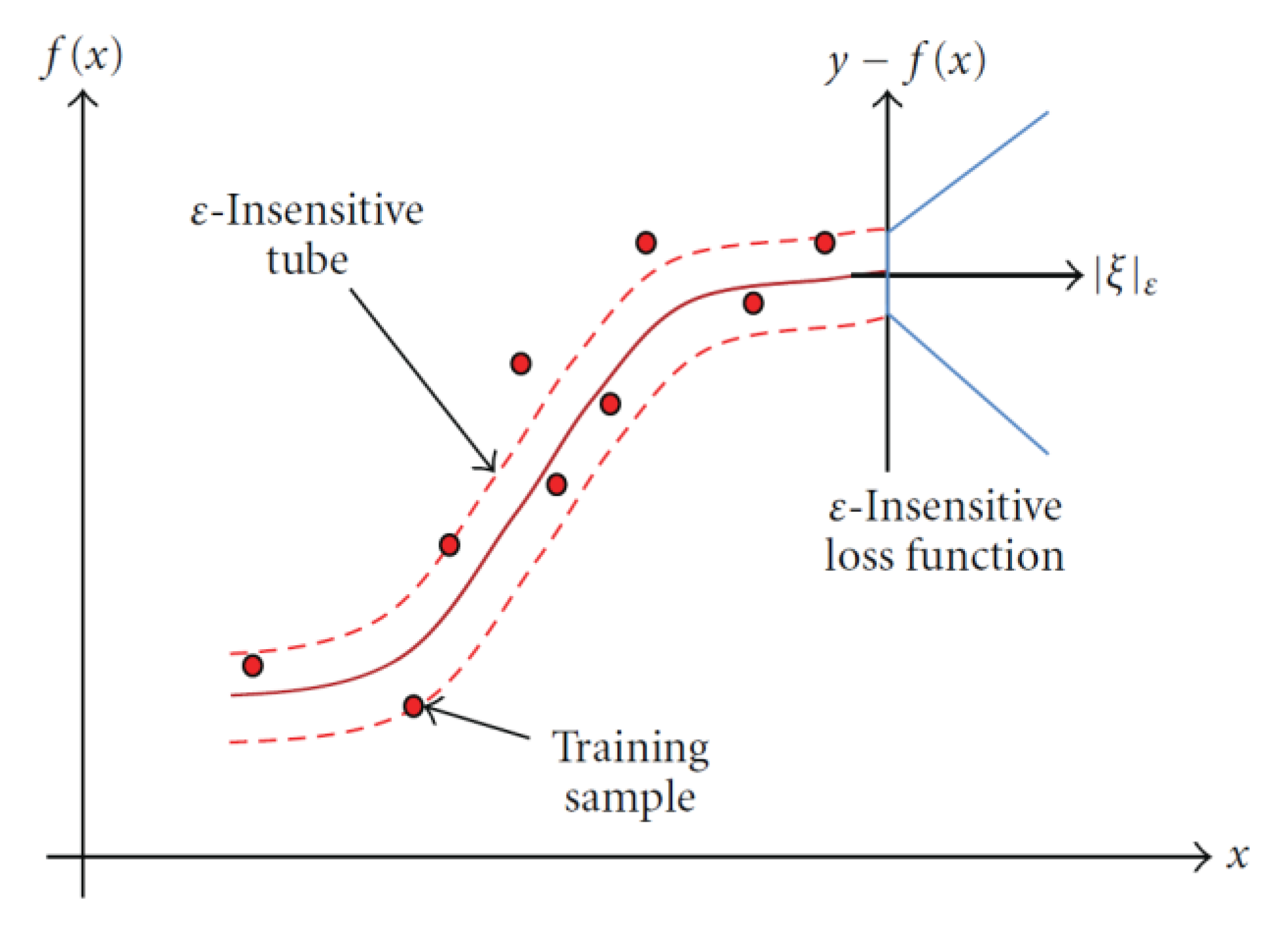
3.2. SVR
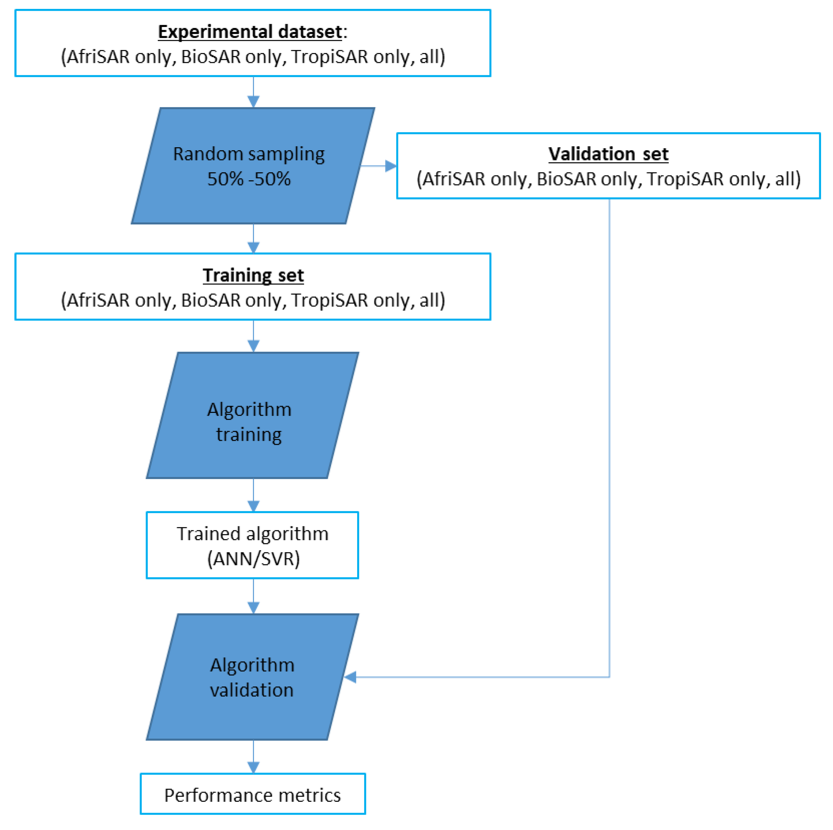
4. Data Analysis
5. Results
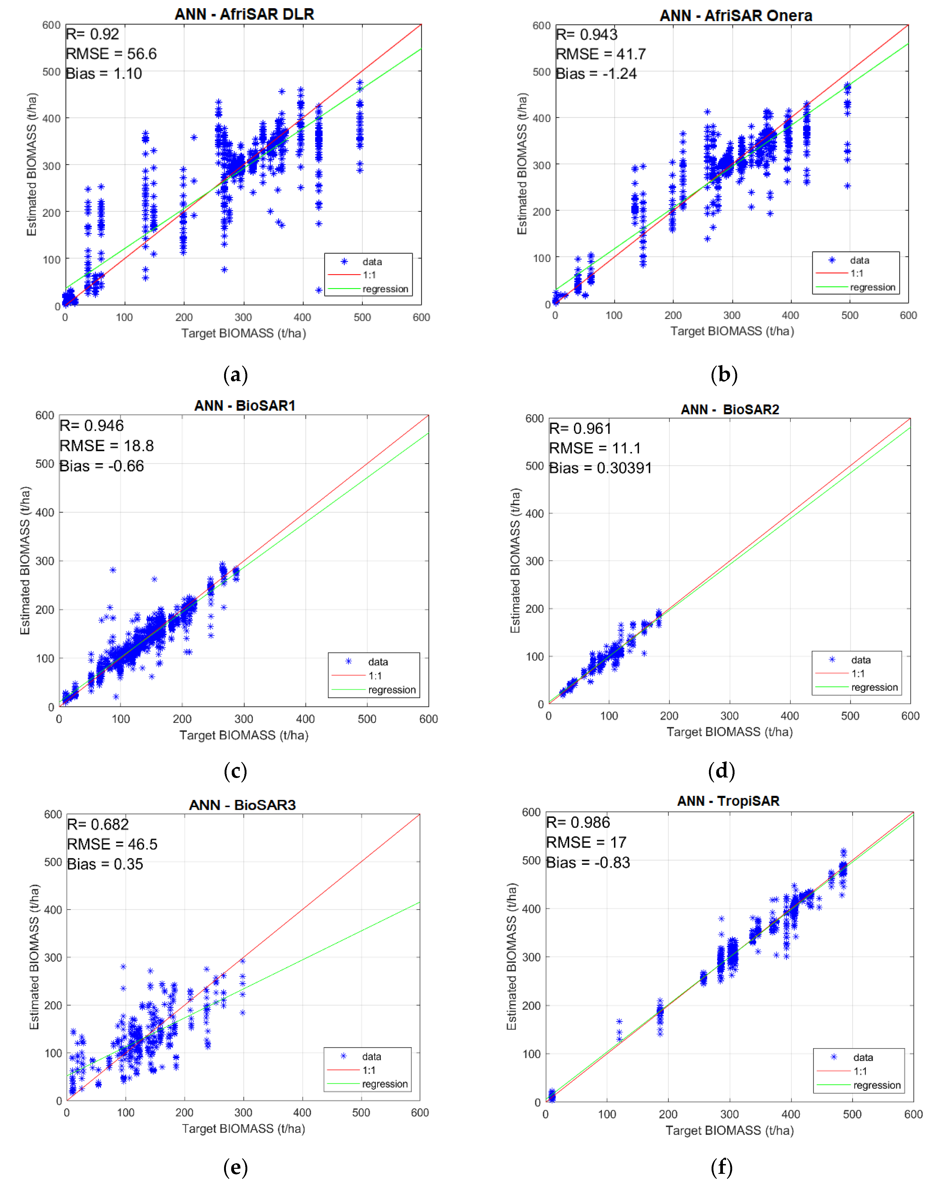
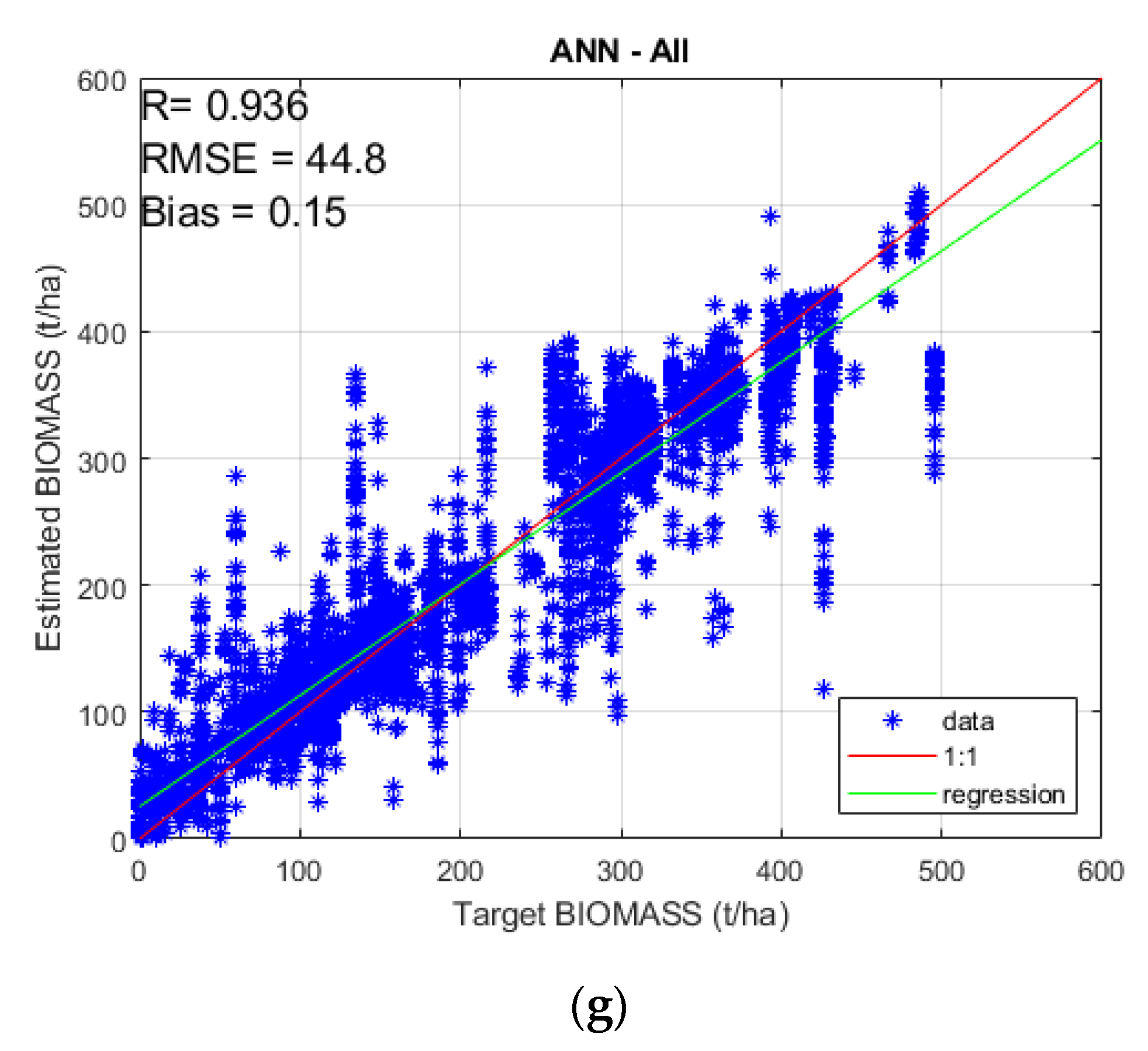
5.1. ANN
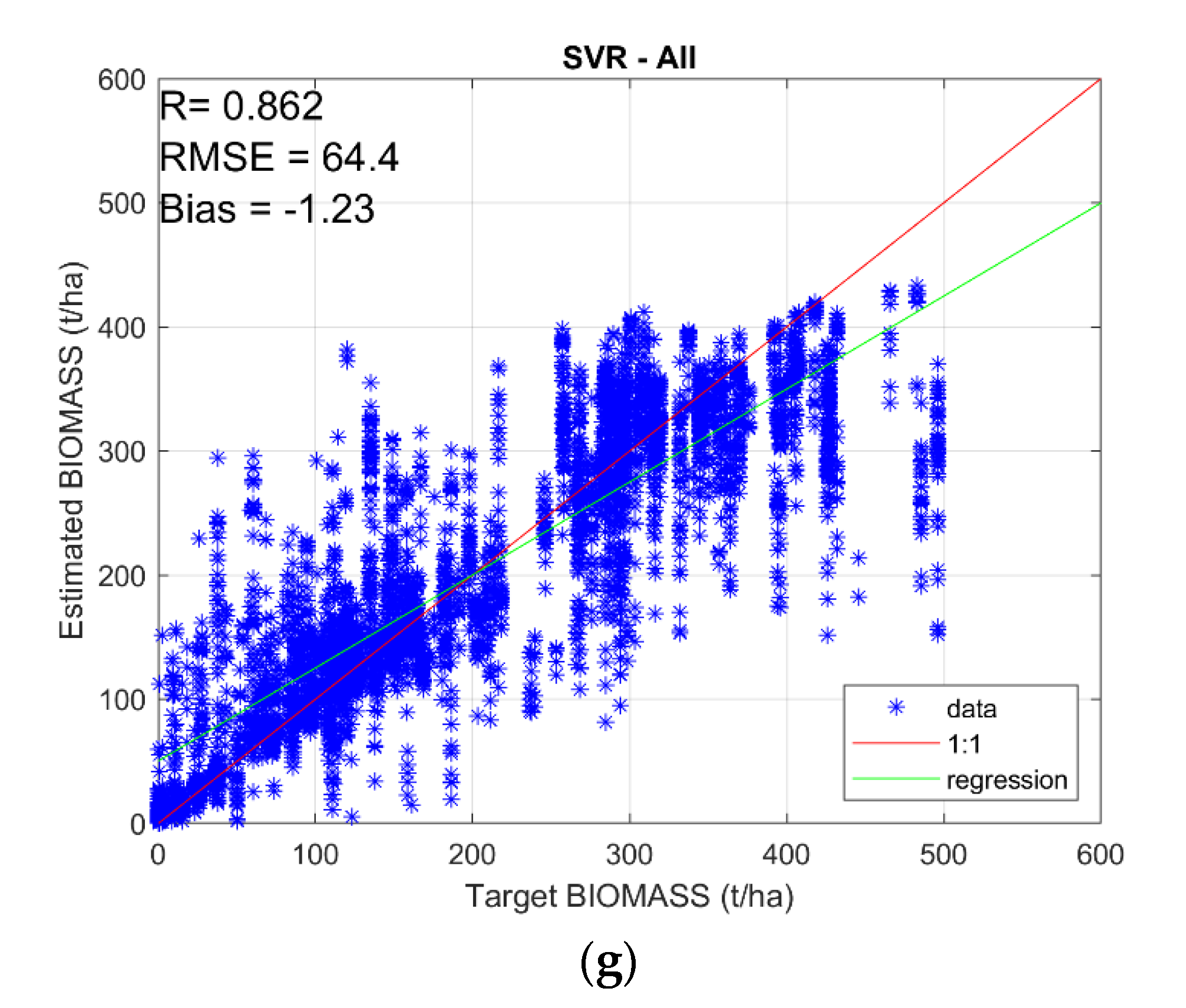
5.2. SVR
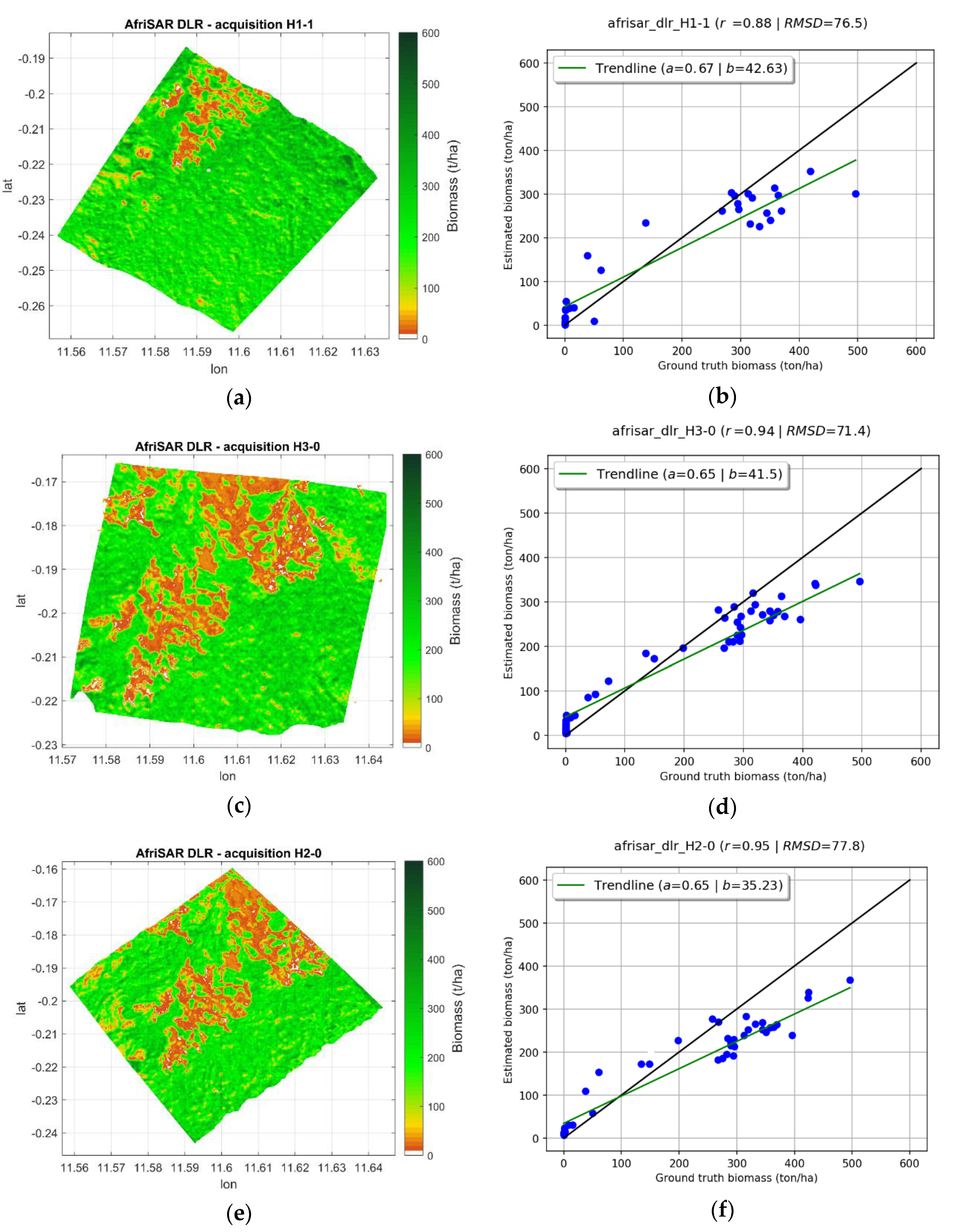
5.3. Biomass Maps
6. Discussion
7. Conclusions and Future Work
Author Contributions
Funding
Acknowledgments
Conflicts of Interest
References
- Waring, H.R.; Running, S.W. Forest Ecosystems. Analysis at Multiples Scales, 3rd ed.; Academic Press: San Diego, CA, USA, 2007. [Google Scholar]
- Le Toan, T.; Laur, H.; Mougin, E. Multitemporal and dualpolarization observations of agricultural vegetation covers by X-band SAR images. IEEE Trans. Geosci. Remote Sens. 1989, 27, 709–718. [Google Scholar] [CrossRef]
- Ulaby, F.T.; Dobson, M.C. Handbook of Radar Statistics for Terrain; Artech House: Norwood, MA, USA, 1989. [Google Scholar]
- Wang, Y.; Kasischke, E.S.; Melack, J.M.; Davis, F.W.; Christensen, N.L. The effects of changes in loblolly pine biomass and soil moisture on ERS-1 SAR backscatter. Remote Sens. Environ. 1994, 49, 25–31. [Google Scholar] [CrossRef]
- Wang, Y.; Hess, L.H.; Filoso, S.; Melack, J.M. Understanding the radar backscattering from flooded and nonflooded Amazonian forests: Results from canopy backscatter modeling. Remote Sens. Environ. 1995, 54, 324–332. [Google Scholar] [CrossRef]
- Ranson, K.J.; Sun, G. Mapping biomass of a northern forest using multifrequency SAR data. IEEE Trans. Geosci. Remote Sens. 1994, 32, 388–396. [Google Scholar] [CrossRef]
- Paloscia, S.; Macelloni, G.; Pampaloni, P.; Sigismondi, S. The Potential of L- and C-Band SAR in Estimating Vegetation Biomass: The ERS-1 and JERS-1 Experiments. IEEE Trans. Geosci. Remote Sens. 1999, 37, 4. [Google Scholar] [CrossRef]
- Kasischke, E.S.; Melack, J.M.; Dobson, M.C. The use of imaging radars for ecological applications—A review. Remote Sens. Environ. 1997, 59, 141–156. [Google Scholar] [CrossRef]
- Ackermann, N.; Thiel, C.; Borgeaud, M.; Schmullius, C. Cosmo-SkyMed backscatter intensity and interferometric coherence signatures over Germany’s low mountain range forested areas. In Proceedings of the Geoscience and Remote Sensing Symposium (IGARSS2012), Munich, Germany, 22–27 July 2012. [Google Scholar] [CrossRef]
- Kaasalainen, S.; Holopainen, M.; Karjalainen, M.; Vastaranta, M.; Kankare, V.; Karila, K.; Osmanoglu, B. Combining LiDAR and Synthetic Aperture Radar Data to Estimate Forest Biomass: Status and Prospects. Forests 2015, 6, 252. [Google Scholar] [CrossRef]
- Baghdadi, N.; Le Maire, G.; Bailly, J.-S.; Osé, K.; Nouvellon, Y.; Zribi, M.; Lemos, C.; Hakamada, R. Evaluation of ALOS/PALSAR L-Band Data for the Estimation of Eucalyptus Plantations Aboveground Biomass in Brazil. IEEE J. Sel. Top. Appl. Earth Obs. Remote Sens. 2015, 8, 2015. [Google Scholar] [CrossRef] [Green Version]
- Dobson, M.C.; Ulaby, F.T.; Le Toan, T.; Beaudoin, A.; Kasischke, E. Dependence of radar backscatter on coniferous forest biomass. IEEE Trans. Geosci. Remote Sens. 1992, 30, 412–415. [Google Scholar] [CrossRef]
- Le Toan, T.; Beaudoin, A.; Riom, J.; Guyon, D. Relating forest biomass to SAR data. IEEE Trans. Geosci. Remote Sens. 1992, 30, 403–411. [Google Scholar] [CrossRef]
- Le Toan, T.; Quegan, S.; Woodward, F.I.; Lomas, M.R.; Delbart, N. Relating radar remote sensing of biomass to modelling of forest carbon budgets. Clim. Chang. 2004, 67, 379–402. [Google Scholar] [CrossRef]
- Ferrazzoli, P.; Paloscia, S.; Pampaloni, P.; Schiavon, G.; Sigismondi, S.; Solimini, D. The potential of multifrequency polarimetric SAR in assessing agricultural and arboreous biomass. IEEE Trans. Geosci. Remote Sens. 1997, 35, 5–179. [Google Scholar] [CrossRef]
- Joshi, N.; Mitchard, E.T.A.; Brolly, M.; Schumacher, J.; Fernández-Landa, A.; Johannsen, V.K.; Marchamalo, M.; Fensholt, R. Understanding ‘saturation’ of radar signals over forests. Sci. Rep. 2017, 7, 3505. [Google Scholar] [CrossRef] [PubMed] [Green Version]
- Mermoz, S.; Réjou-Méchain, M.; Villard, L.; le Toan, T.; Rossi, V.; Gourlet-Fleury, S. Decrease of L-band SAR backscatter with biomass of dense forests. Remote Sens. Environ. 2015, 159, 307–317. [Google Scholar] [CrossRef]
- Saatchi, S.S.; Moghaddam, M. Estimation of crown and stem water content and biomass of boreal forest using polarimetric SAR imagery. IEEE Trans. Geosci. Remote Sens. 2000, 38, 697–709. [Google Scholar] [CrossRef] [Green Version]
- Moghaddam, M.; Saatchi, S.; Cuenca, R.H. Estimating subcanopy soil moisture with radar. J. Geophys. Res. 2000, 105, 14899. [Google Scholar] [CrossRef] [Green Version]
- Le Toan, T.; Quegan, S.; Davidson, M.; Balzter, H.; Paillou, P.; Papathanassiou, K.; Plummer, S.; Saatchi, S.; Shugart, H.; Ulander, L. The BIOMASS Mission: Mapping global forest biomass to better understand the terrestrial carbon cycle. Remote Sens. Environ. 2011, 115, 2850–2860. [Google Scholar] [CrossRef] [Green Version]
- Christian, N.; Watanabe, M.; Hayashi, M.; Ogawa, T.; Shimada, M. Mapping the spatial-temporal variability of tropical forests by ALOS-2 L-band SAR big data analysis. Remote Sens. Environ. 2019, 233, 111372. [Google Scholar] [CrossRef]
- Sandberg, G.; Ulander, L.M.H.; Fransson, J.E.S.; Holmgren, J.; Le Toan, T. L- and P-band backscatter intensity for biomass retrieval in hemiboreal forest. Remote Sens. Environ. 2011, 115, 2874–2886. [Google Scholar] [CrossRef]
- Saatchi, S.; Marlier, M.; Chazdon, R.L.; Clark, D.B.; Russell, A.E. Impact of spatial variability of tropical forest structure on radar estimation of aboveground biomass. Remote Sens. Environ. 2011, 115, 2836–2849. [Google Scholar] [CrossRef]
- Cazcarra-Bes, V.; Tello-Alonso, M.; Fischer, R.; Heym, M.; Papathanassiou, K. Monitoring of Forest Structure Dynamics by Means of L-Band SAR Tomography. Remote Sens. 2017, 9, 1229. [Google Scholar] [CrossRef] [Green Version]
- Blomberg, E.; Ferro-Famil, L.; Soja, M.J.; Ulander, L.M.H.; Tebaldini, S. Forest Biomass Retrieval from L-Band SAR Using Tomographic Ground Backscatter Removal. IEEE Geosci. Remote Sens. Lett. 2018, 15, 1030–1034. [Google Scholar] [CrossRef]
- Notarnicola, C. A Bayesian Change Detection Approach for Retrieval of Soil Moisture Variations under Different Roughness Conditions. IEEE Geosci. Remote Sens. Lett. 2014, 11, 414–418. [Google Scholar] [CrossRef]
- Pasolli, L.; Notarnicola, C.; Bruzzone, L. Estimating soil moisture with the support vector regression technique. IEEE Geosci. Remote Sens. Lett. 2011, 8, 1080–1084. [Google Scholar] [CrossRef]
- Pierdicca, N.; Pulvirenti, L.; Pace, G. A Prototype Software Package to Retrieve Soil Moisture from Sentinel-1 Data by Using a Bayesian Multitemporal Algorithm. IEEE J. Sel. Top. Appl. Earth Obs. Remote Sens. 2014, 7, 153–163. [Google Scholar] [CrossRef]
- Del Frate, F.; Ferrazzoli, P.; Schiavon, G. Retrieving soil moisture and agricultural variables by microwave radiometry using neural networks. Remote Sens. Environ. 2003, 84, 174–183. [Google Scholar] [CrossRef]
- Paloscia, S.; Pampaloni, P.; Pettinato, S.; Santi, E. A comparison of algorithms for retrieving soil moisture from ENVISAT/ASAR images. IEEE Tran. Geosci. Remote Sens. 2008, 46, 3274–3284. [Google Scholar] [CrossRef]
- Paloscia, S.; Pettinato, S.; Santi, E.; Notarnicola, C.; Pasolli, L.; Reppucci, A. Soil moisture mapping using Sentinel-1 images: Algorithm and preliminary validation. Remote Sens. Environ. 2013, 134, 234–248. [Google Scholar] [CrossRef]
- Santi, E.; Paloscia, S.; Pettinato, S.; Fontanelli, G. Application of artificial neural networks for the soil moisture retrieval from active and passive microwave spaceborne sensors. Int. J. Appl. Earth Obs. Geoinf. 2016, 48, 61–73. [Google Scholar] [CrossRef]
- Santi, E.; Paloscia, S.; Pettinato, S.; Chirici, G.; Mura, M.; Maselli, F. Application of Neural Networks for the retrieval of forest woody volume from SAR multifrequency data at L and C bands. Eur. J. Remote Sens. 2015, 48, 673–687. [Google Scholar] [CrossRef] [Green Version]
- Santi, E.; Paloscia, S.; Pettinato, S.; Fontanelli, G.; Mura, M.; Zolli, C.; Maselli, F.; Chiesi, M.; Bottai, L.; Chirici, G. The potential of multifrequency SAR images for estimating forest biomass in Mediterranean areas. Remote Sens. Environ. 2017, 200, 63–73. [Google Scholar] [CrossRef]
- Evgeniou, T.; Pontil, M.; Poggio, T. Regularization Networks and Support Vector Machines. Adv. Comput. Math. 2000, 13, 1–50. [Google Scholar] [CrossRef]
- Smola, A.J.; Schölkopf, B. A tutorial on support vector regression. Stat. Comput. 2004, 14, 199–222. [Google Scholar] [CrossRef] [Green Version]
- Pasolli, L.; Notarnicola, C.; Bruzzone, L.; Bertoldi, G.; Della Chiesa, S.; Hell, V.; Niedrist, G.; Tappeiner, U.; Zebisch, M.; Del Frate, F.; et al. Estimation of Soil Moisture in an Alpine Catchment with RADARSAT2 Images. Hindawi Publishing Corporation. Appl. Environ. Soil Sci. 2011. [Google Scholar] [CrossRef]
- Fatoyinbo, L.; Pinto, N.; Hofton, M.; Simard, M.; Blair, B.; Saatchi, S.; Lou, Y.; Dubayah, R.; Hensley, S.; Armston, J.; et al. The 2016 NASA AfriSAR campaign: Airborne SAR and Lidar measurements of tropical forest structure and biomass in support of future satellite missions. In Proceedings of the 2017 IEEE International Geoscience and Remote Sensing Symposium (IGARSS), Fort Worth, TX, USA, 23–28 July 2017; pp. 4286–4287. [Google Scholar] [CrossRef]
- Hajnsek, I.; Scheiber, R.; Lee, S.; Ulander, L.; Gustavsson, A.; Tebaldini, S.; Monte Guarnieri, A. BioSAR 2007. Technical Assistance for the Development of Airborne SAR and Geophysical Measurements during the BioSAR 2007 Experiment: Final Report without Synthesis. Ph.D. Thesis, European Space Agency, Paris, France, 2008. [Google Scholar]
- Hajnsek, I.; Scheiber, R.; Keller, M.; Horn, R.; Lee, S.; Ulander, L.; Gustavsson, A.; Sandberg, G.; le Toan, T.; Tebaldini, S.; et al. BioSAR 2008. Technical assistance for the development of airborne SAR and geophysical measurements during the BioSAR 2008 Experiment DRAFT Final Report-BIOSAR Campaign. Ph.D. Thesis, European Space Agency, Paris, France, 2009. [Google Scholar]
- Ulander, L.M.; Gustavsson, A.; Dubois-Fernandez, P.; Dupuis, X.; Fransson, J.E.; Holmgren, J.; Wallerman, J.; Eriksson, L.; Sandberg, G.; Soja, M. Proceedings of the 2011 IEEE International Geoscience and Remote Sensing Symposium, Vancouver, BC, Canada, 25–29 July 2011.
- Dubois-Fernandez, P.; Oriot, H.; Coulombeix, C.; Cantalloube, H.; du Plessis, O.R.; Le Toan, T.; Daniel, S.; Chave, J.; Blanc, L.; Davidson, M. TropiSAR a SAR data acquisition campaign in French Guiana. In Proceedings of the 8th European Conference on Synthetic Aperture Radar, Aachen, Germany, 7–10 June 2010; pp. 1074–1077. [Google Scholar]
- Dubois-Fernandez, P.; Le Toan, T.; Chave, J.; Blanc, L.; Daniel, S.; Oriot, H.; Arnaubec, A.; Réjou-Méchain, M.; Villard, L.; Lasne, Y.; et al. Technical Assistance for the Development of Airborne SAR and Geophysical Measurements during the TropiSAR 2009 Experiment: Final Report; TROPISAR-Final Report, ESA CONTRACT N° 22446/09/NL/CT; European Space Agency: Paris, France, February 2011. [Google Scholar]
- Mladenova, I.E.; Jackson, T.J.; Bindlish, R.; Hensley, S. Incidence Angle Normalization of Radar Backscatter Data. IEEE Trans. Geosci. Remote Sens. 2013, 51, 1791–1804. [Google Scholar] [CrossRef]
- Villard, L.; le Toan, T. Relating P-Band SAR Intensity to Biomass for Tropical Dense Forests in Hilly Terrain: γ0ort0. IEEE J. Sel. Top. Appl. Earth Obs. Remote Sens. 2015, 8, 214–223. [Google Scholar] [CrossRef]
- van Zyl, J.J. The effect of topography on radar scattering from vegetated areas IEEE Trans. Geosci. Remote Sens. 1993, 31, 153–160. [Google Scholar] [CrossRef]
- Schlund, M.; Davidson, M.W.J. Aboveground Forest Biomass Estimation Combining L- and P-Band SAR Acquisitions. Remote Sens. 2018, 10, 1151. [Google Scholar] [CrossRef] [Green Version]
- Available online: https://earth.esa.int/web/sppa/meetings-workshops/hosted-and-co-sponsored-meetings/brix (accessed on 26 February 2020).
- Hornik, K. Multilayer feed forward network are universal approximators. Neural Netw. 1989, 2, 359–366. [Google Scholar] [CrossRef]
- Linden, A.; Kinderman, J. Inversion of multi-layer nets. Proc. Int. Joint Conf. Neural Netw. 1989, 2, 425–443. [Google Scholar]
- Bruzzone, L.; Melgani, F. Robust multiple estimator system for the analysis of biophysical parameters from remotely sensed data. IEEE Trans. Geosci. Remote Sens. 2005, 43, 159–174. [Google Scholar] [CrossRef]
- Pasolli, L.; Notarnicola, C.; Bertoldi, G.; Bruzzone, L.; Remelgado, R.; Greifeneder, F.; Niedrist, G.; Della Chiesa Tappeiner, U.; Zebisch, M. Estimation of Soil Moisture in Mountain Areas Using SVR Technique Applied to Multiscale Active Radar Images at C-Band. IEEE J. Sel. Top. Appl. Earth Obs. Remote Sens. 2015. [Google Scholar] [CrossRef]
- Vapnik, V. The Nature of Statistical Learning Theory; Springer: New York, NY, USA, 1995. [Google Scholar]
- Santoro, M.; Eriksson, L.; Askne, J.; Schmullius, C. Assessment of stand-wise stem volume retrieval in boreal forest from JERS-1 L-band SAR backscatter. Int. J. Remote Sens. 2006, 27, 3425–3454. [Google Scholar] [CrossRef]
- Attema, E.P.W.; Ulaby, F.T. Vegetation modeled as a water cloud. Radio Sci. 1978, 13, 357–364. [Google Scholar] [CrossRef]


| Campaign | RVV | RVH | RHV | RHH |
|---|---|---|---|---|
| AfriSAR DLR | 0.74 | 0.76 | 0.76 | 0.64 |
| AfriSAR Onera | 0.51 | 0.64 | 0.65 | 0.53 |
| BioSAR 1 | 0.07 | 0.21 | 0.21 | 0.35 |
| BioSAR 2 | −0.04 | 0.04 | 0.03 | 0.05 |
| BioSAR 3 | 0.02 | −0.01 | 0 | 0.02 |
| TropiSAR | 0.5 | 0.69 | 0.68 | 0.27 |
| All | 0.05 | 0.23 | 0.23 | 0.06 |
© 2020 by the authors. Licensee MDPI, Basel, Switzerland. This article is an open access article distributed under the terms and conditions of the Creative Commons Attribution (CC BY) license (http://creativecommons.org/licenses/by/4.0/).
Share and Cite
Santi, E.; Paloscia, S.; Pettinato, S.; Cuozzo, G.; Padovano, A.; Notarnicola, C.; Albinet, C. Machine-Learning Applications for the Retrieval of Forest Biomass from Airborne P-Band SAR Data. Remote Sens. 2020, 12, 804. https://doi.org/10.3390/rs12050804
Santi E, Paloscia S, Pettinato S, Cuozzo G, Padovano A, Notarnicola C, Albinet C. Machine-Learning Applications for the Retrieval of Forest Biomass from Airborne P-Band SAR Data. Remote Sensing. 2020; 12(5):804. https://doi.org/10.3390/rs12050804
Chicago/Turabian StyleSanti, Emanuele, Simonetta Paloscia, Simone Pettinato, Giovanni Cuozzo, Antonio Padovano, Claudia Notarnicola, and Clement Albinet. 2020. "Machine-Learning Applications for the Retrieval of Forest Biomass from Airborne P-Band SAR Data" Remote Sensing 12, no. 5: 804. https://doi.org/10.3390/rs12050804
APA StyleSanti, E., Paloscia, S., Pettinato, S., Cuozzo, G., Padovano, A., Notarnicola, C., & Albinet, C. (2020). Machine-Learning Applications for the Retrieval of Forest Biomass from Airborne P-Band SAR Data. Remote Sensing, 12(5), 804. https://doi.org/10.3390/rs12050804