Attention-Guided Multi-Scale Segmentation Neural Network for Interactive Extraction of Region Objects from High-Resolution Satellite Imagery

Abstract

Automatic extraction of region objects from high-resolution satellite imagery presents a great challenge, because there may be very large variations of the objects in terms of their size, texture, shape, and contextual complexity in the image. To handle these issues, we present a novel, deep-learning-based approach to interactively extract non-artificial region objects, such as water bodies, woodland, farmland, etc., from high-resolution satellite imagery. First, our algorithm transforms user-provided positive and negative clicks or scribbles into guidance maps, which consist of a relevance map modified from Euclidean distance maps, two geodesic distance maps (for positive and negative, respectively), and a sampling map. Then, feature maps are extracted by applying a VGG convolutional neural network pre-trained on the ImageNet dataset to the image X, and they are then upsampled to the resolution of X. Image X, guidance maps, and feature maps are integrated as the input tensor. We feed the proposed attention-guided, multi-scale segmentation neural network (AGMSSeg-Net) with the input tensor above to obtain the mask that assigns a binary label to each pixel. After a post-processing operation based on a fully connected Conditional Random Field (CRF), we extract the selected object boundary from the segmentation result. Experiments were conducted on two typical datasets with diverse region object types from complex scenes. The results demonstrate the effectiveness of the proposed method, and our approach outperforms existing methods for interactive image segmentation.

1. Introduction

With the advances in high-resolution satellite remote sensing technology, a huge number of aerial images are being collected, presenting new challenges to geographic information workers. Image interpretation is an important research area in the remote sensing field as the results are used for various applications such as digital mapping, urbanization monitoring, land use monitoring, and resource environment [1]. Assigning a corresponding classification label to each pixel of a satellite image is one of the most important image interpretation tasks. How to extract region objects from high-resolution remote sensing images effectively and quickly is a big challenge, which has received much attention in recent years. Although many scholars have done a lot of research on automatic interpretation, most of the methods remain in the experimental stage [2]. Due to the complexity of the problem, the approach based on computer-automated interpretation could not meet the production requirements in a short time. The practical application mainly depends on manual interpretation, which requires a lot of manpower and material resources. In fact, semi-automatic interpretation (also called interactive extraction) can obtain a much better result with only a small amount of manual operation required [3].

Interactive extraction uses the constraints provided by the user and the prior knowledge of targets to guide the processing process. A good interactive extraction algorithm should be able to obtain the accurate mask of the target object with less user effort. In the field of computer vision, various interactive extraction algorithms emerge one after another, which also play important roles in the area of object extraction from satellite images. In consideration of feature extraction and model characteristics, the classical interactive methods of region object extraction can be summed up into two categories: methods based on boundary and methods based on region [4]. The methods based on boundary require users to specify the approximate position or provide a few key points of the boundary, and then take the characteristics of boundary strength and continuity into account to track the smooth boundary. For instance, Fazana et al. [5] presented a building extraction algorithm combining a Snake model and dynamic programming. The user was only required to specify several seed points at the corner of the room, indicating the approximate position of the building, and the algorithm then extracted an accurate contour of the building. The methods based on region require users to roughly specify some seed points or scribbles in the target or background area, and then the algorithm calculates the category for other unclassified areas of the image according to these seed points or scribbles through certain strategies. For instance, Osman et al. [6] proposed a building extraction algorithm combining the SVM model and region growing. From two sets of pixels sampled by the user, a binary mask was produced to represent the selected object. However, non-artificial region objects, which always refer to water, woodland, farmland, bare land and so on, have no artificial intervention. Given that such natural objects are hugely irregular in size and shape, these methods mentioned above, using limited information under several assumptions, do not have the ability to extract accurate and appropriate features.

Deep learning methods, with strong supervision, have been gradually dominating the fields of computer vision over the past few years. Various methods are presented to speed up the process of developments of image classification (AlexNet, GoogleNet, VGG, ResNet [7,8,9,10]), object detection (R-CNN, Fast R-CNN, Faster R-CNN, Mask R-CNN, YOLO, SSD [11,12,13,14,15,16]), image segmentation (U-Net, FCN, PSPNet, SegNet, DeepLab [17,18,19,20,21]), and other computer vision tasks. An obvious strategy is adapting these successful networks to imagery interpretation tasks. Saito et al. [22] proposed using CNNs, including feature extraction and classifiers, to automatically extract roads and buildings. The proposed method took pixel values in aerial imagery as the input and predicted a three-channel mask (road, building, background). Kussul et al. [23] compared CNNs with traditional multilayer perceptron and random forest, confirming the result of CNNs to be superior to traditional methods. A semantic segmentation method was proposed in [24], which initialized a CNN framework by substituting real MSI imagery for generated synthetic MSI imagery.

The existing methods based on CNNs remain in the experimental stage, and could not guarantee the accuracy of the object extraction result in an automatic pattern. In addition, vast amounts of label-data are required for model training, but the model still has the problem of insufficient generalization in the face of various types of images. Some medical scholars and computer scientists have proposed the combination of user-interactions and deep learning to solve the extraction problem. Xu et al. [25] proposed a deep interactive object selection method. User-provided clicks were transformed into two positive and negative Euclidean distance maps, which were then concatenated with the raw image as the input of the Fully Convolutional Networks (FCN [18]). In [26], user-provided bounding boxes were employed as weak-annotations to train CNNs for the task of medical image segmentation. DeepIGeoS [27] got an automatic segmentation result using a coarse decoder, which was then refined by a fine decoder that took user-scribbles and the coarse segmentation mask as input. Li et al. [28] presented a selection network to sort the segmentation results conforming to the user’s interactions. Given that the interactive extraction of objects from satellite imagery is totally different from the interactive extraction of objects in natural images, we must take lots of impacts into consideration in more complex scenes. However, only a few frameworks have been proposed to apply CNNs to interactive satellite imagery interpretation [29].

The task of satellite imagery interpretation is to assign a semantic label to each pixel of the input image, which is similar to the semantic segmentation in the domain of computer vision. Lots of work have been done to bring the tricks, skills, and strategies in the domain of computer vision to the task of satellite imagery interpretation, which have achieved good performance recently. However, there are still some limitations of the approaches in the face of practical applications. Song et al. [30] was inspired by an Itti visual attention model for natural image processing and proposed a method of object contour extraction from satellite imagery using the Snake model based on the selected salient regions. This strategy could work well in situations where the background is easily distinguishable but would fail when salient regions cannot be extracted effectively. In our work, we used the pre-trained CNNs model to extract robust features instead of using unstable salient regions. In [31], a method of counting built-structures in the satellite imagery was proposed by combining features from different regions using attention-based reweighting techniques. However, different from the regular and well-bound artificial buildings, non-artificial region objects in terms of their various shapes, sizes, textures, and contextual complexities are hard to be distinguished without any guidance. In our work, we introduced user-interactions into the CNNs to guide the framework to segment the specific target object. Xu et al. [32] proposed an ingenious network that incorporates control gate and feedback attention mechanisms to perform pixel-wise classification for satellite imagery. This approach does use ingenious designs to achieve good performance for the automatic satellite imagery interpretation while it needs long processing time. An interactive interpretation system considers not only the accuracy but also the response time, which means the users cannot wait too long after putting a new seed to the system. Thus, we replaced the control gate and feedback attention mechanisms by a combination of two channel-wise attention mechanisms and took scale viability problem into account to avoid loss of information. These strategies help the proposed system meet the real-time requirements in the task of interactive satellite imagery interpretation, which also apply to the domain of computer vision.

With the good performance of interactive image segmentation in the domain of computer vision [33,34,35] and the limitations of the current automatic interpretation [30,31,32], we propose a novel method for deep interactive extraction of non-artificial region objects. In this approach, user-provided interactions (clicks, scribbles) are first transformed into the guidance maps G. Then, we apply a VGG [9] network pre-trained on the ImageNet dataset to the input image X, to effectively extract the feature maps F from the complex background. We concatenate image X, guidance maps G, and feature maps F as the input tensor, which is fed into the attention-guided multi-scale segmentation network to obtain the binary mask. Finally, we integrate the binary mask into the CRF optimization to extract the accurate boundary of the selected object. We evaluate our approach using two complex datasets with diverse non-artificial region object types. The experimental results show that our approach is superior to other existing methods.

The main contributions of this paper are summarized as follows:

• To effectively and simply simulate the user-provided interactions of selecting the region object, our algorithm not only adopts the click-based interaction but also supports the scribble-based interaction. We provide a more flexible and suitable interactive mechanism for the users to select the appropriate way of interactions based on a certain scene.
• To take the image context and appearance into consideration, we propose an effective transformation of user-provided interactions to obtain the guidance maps. We combine the modified Euclidean distance transformation, sampling transformation, and geodesic distance transformation to avoid the rich information loss, which is caused by using only the simple Euclidean distance transformation adopted by existing methods.
• We present a novel way to incorporate user-interactions and convolutional neural networks, using the guidance maps as extra channels of the input of the segmentation network. It is the first work to adopt this special mechanism to the interactive extraction of region objects from satellite imagery.
• With our proposed attention-guided multi-scale segmentation network that can focus the special channels and take multi-scale information into account, we achieve higher segmentation accuracy with fewer user interactions compared with other interactive methods.

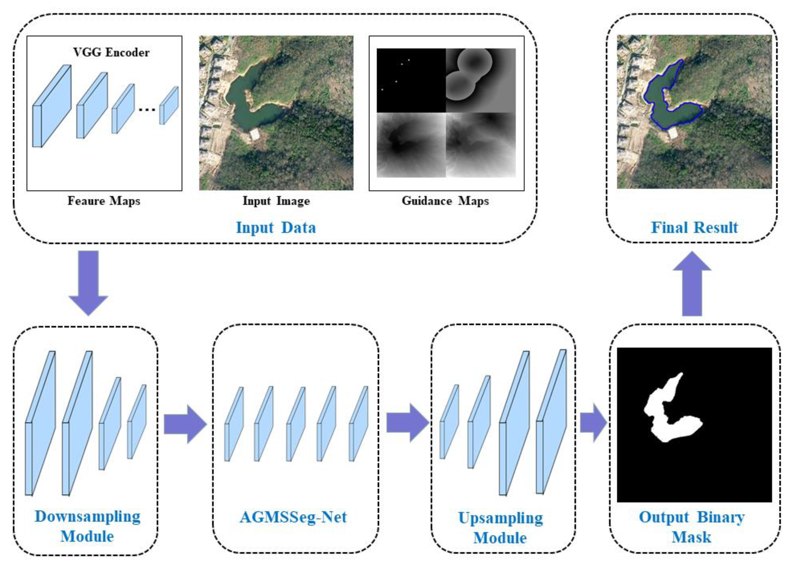
The remainder of this article is arranged as follows: Section 2 describes details of the proposed method; the corresponding experimental assessment and discussion of the obtained results are shown in Section 3 and Section 4, respectively; Section 5 presents our concluding remarks.

2. Methodology

A novel region object extraction approach based on deep interactive segmentation from high-resolution remote sensing images is presented in this work, and Figure 1 illustrates the schematic architecture of the presented method. To implement the entire framework, the presented method is composed of three parts: generation of the guidance maps (Section 2.1), attention-guided multi-scale segmentation network (Section 2.2), and post-processing for final region object extraction (Section 2.3).

2.1. Generation of Guidance Maps

We incorporate user interactions and CNNs by transforming the sampling into several binary maps. Given the method based on deep learning we used in this paper, the model requires a great number of training pairs consisting of images and guidance maps. In the learning stage, we cannot collect sufficient interaction sequences provided by real users. Therefore, inspired by Xu’s work [25], we propose a strategy that simulates user random sampling based on clicks and scribbles. In the prediction stage, the interaction information is provided by gradually adding a click or scribble to the input image. Then, a simple yet powerful interaction transformation approach, using several distance-calculating algorithms, is adopted to generate the guidance maps.

2.1.1. Simulating User Sampling

To simulate user interaction sequences, we generate positive and negative clicks or scribbles for corresponding labels, respectively, with automatic random sampling. Since region objects in satellite images are irregular in size and shape, the random sampling based only on clicks is too limited to cover all the objects of various sizes (as shown in Figure 2, ponds and rivers differ greatly in size and shape). On the one hand, the sampling based on scribbles covers more pixels than that based on clicks, which means the former provides more information in complex and large-scale scenes for imagery interpretation. On the other hand, the sampling based on clicks is more suitable in clear and small-scale scenes because of the advantages of simplicity and convenience. In order to combine the advantages of both sampling strategies, interactions based on clicks and scribbles are both supported to adapt to different scenes.

For random click sampling, we follow the sampling strategies proposed in [25]. To sample positive clicks, we randomly sampled $N_{pos}^c$ clicks within the selected object. Two hard-constraints were applied to click location selection, one in which every click was at least $d_1$ pixels away from the object boundary and the other in which every click was $d_2$ pixels away from each other. To sample negative clicks, two of the three strategies were adopted: one was random sampling $N_{neg}^{c1}$ clicks within the background added to the same hard-constraints as the positive sampling, the other was random sampling $N_{neg}^{c2}$ clicks around the selected object boundary.

For random scribble sampling, we first present a simple method using a skeletonization algorithm [36] to obtain a small set of pixels with the same label from the ground truth. First, we obtained each object instance from the ground truth mask by ensuring that the selected object has the feature of connectivity in a $4\times 4$ neighborhood. After adopting the skeletonization algorithm, a scribble of one-pixel-wise presenting the area of the selected object instance was obtained. The skeletonization algorithm used morphological thinning that erodes away pixels from the boundary until no more thinning is possible, at which point what is left approximates the skeleton. Finally, we expanded the width of the scribble to cover more pixels, which means more corresponding semantic labels are set correctly, to make full use of information that the users can provide.

In the test stage, we do not need to take the complexity of the scribble generation algorithm into account, because scribbles are provided by the user directly. In the training stage, we should guarantee the algorithm is sufficiently robust to exactly select the target object. As scribble generated by the skeletonization algorithm could cover most of the areas of the target, no more scribbles were required to select the object. Therefore, we set the number of positive scribbles $N_{pos}^s$ to 1. To sample negative scribbles, [29] proposed a “background scribble generation” method via Random Walks. Different from their works, we simply cut the background scribble into several pieces after inverting the ground truth mask. Then, $N_{neg}^s$ negative scribbles were selected from the pieces after applying the same hard-constraints as the click sampling. The reason why we could do this is that the background is not the area of interest. Scribble generation examples are shown in Figure 3.

2.1.2. Transformation from Interactions to Guidance Maps

By simulating user sampling, we obtain the interaction information with the clicks or scribbles, which labels a specific pixel or a set of pixels as being either “selected object” or “background (region not of interest)”. Then, the interaction information is transformed into guidance maps leading the network to segment the selected object. Euclidean distance transformation (EDT) is a common method to measure the relationship between a pixel (any pixel in the original image) and a set of pixels (sampling set) [25,28,34]. We modified EDT by concatenating a positive and a negative Euclidean distance map after normalization processing. Specifically, since the positive sampling clicks or scribbles were obtained by simulating user interactions, we could use Euclidean distance transformation to generate a positive Euclidean distance map named $E{D}_p$ ($p$ for a positive channel). The same for the obtainment of a negative Euclidean distance map named $E{D}_n$ ($n$ for a negative channel). Then, we recalculated the value of each pixel at the location $\left(i,j\right)$ by using the proposed strategy of combining the two distance maps ($E{D}_p$ and $E{D}_n$), and normalized the combination of the maps to $\left[0,1\right]$. We normalized the relevance map $E\left(v_{i,j}\right)$ to $\left[0,1\right]$ so that it could be concatenated to other guidance maps easily by embedding to other tensors. The relevance map $E\left(v_{i,j}\right)$ is defined as follows:

$$E\left(v_{i,j}\right)=1-\frac{1}{2}\left(E{D}_p\left(v_{i,j}\right)+E{D}_n\left(v_{i,j}\right)\right)$$

(1)

$$E{D}_p\left(v_{i,j}\right)=\underset{\forall v_{m,n}\in S_p}{min}\sqrt{{\left(i-m\right)}^2+{\left(j-n\right)}^2}$$

(2)

$$E{D}_n\left(v_{i,j}\right)=\underset{\forall v_{m,n}\in S_n}{min}\sqrt{{\left(i-m\right)}^2+{\left(j-n\right)}^2}$$

(3)

where $p$ and $n$ represent the positive and negative channel, respectively, $v_{i,j}$ denotes the value of each pixel at the location $\left(i,j\right)$, and $S$ is the set of the specific pixels for positive or negative sampling ($S_p$ for positive channel and $S_n$ for negative channel).

However, limited by the simplicity of its calculation, EDT does not take the image context into account. In addition to taking advantage of spatial constraints, we can also use appearance and semantic contexts. To better utilize image information, Geodesic distance transformation (GDT) [37] was adopted to encode user interactions. Similar to EDT, the geodesic distance map is obtained by:

$$G{D}_t\left(v_{ij}\right)=\underset{\forall u_{m,n}\in S_t}{min}Dis\left(v_{i,j},u_{m,n},I\right),t\in \left\{p,n\right\}$$

(4)

$$Dis\left(v_{i,j},u_{m,n},I\right)=\underset{\forall path\in Pat{h}_{v,u}}{min}{{\displaystyle \int }}_0^1\Vert \nabla I\left(path\left(s\right)\times r\left(s\right)\right)\Vert ds$$

(5)

where $I$ represents the image, $Pat{h}_{v,u}$, $r$, respectively, denote all the paths between pixel $v$ and $u$ and its direction vector, and $\nabla I$ is a difference approximation of the gradient between pixel $v$ and $u$.

As for the sampling map, we simply generated a binary mask, where we set the sampling pixels to 255 while the others were set to 0, both for positive and negative sampling. After all the preparation work was completed, a relevance map, two geodesic distance maps, and a sampling map were concatenated together as the guidance maps. Figure 4 depicts different user-interaction encoding methods.

2.2. Attention-Guided Multi-Scale Segmentation Network

The proposed attention-guided multi-scale segmentation network (AGMSSeg-Net) is different from the prevalent encoder–decoder structure, using dilated convolution [38,39] rather than a pooling operation to grow the receptive field. We adopted multi-scale convolution to handle the scale viability problem by fusing the low-level and high-level feature maps. Given that the interactive segmentation task is obviously influenced by user interactions, the prevalent deep interactive segmentation methods always use the guidance maps to lead the network to segment the target. In addition, the proposed multi-scale segmentation network was configured with an Attention-Guided Convolution (AGC) module to generate a finer mask by focusing on the specific channels and locations. In this section, we first present the AGC module and then describe the multi-scale segmentation network in detail.

2.2.1. Attention-Guided Convolution (AGC) Module

Except for user-provided interactions for selecting desired objects, the interactive segmentation task is similar to the instance segmentation task. Therefore, how do we use the information to make the machine understand the aim to segment the selected object from the complex background? Guiding the network to focus the specific channels and locations, using user sampling, is perhaps a suitable method. Wang et al. [40] proposed a mechanism called scale attention, extracting the feature maps from deep layers to obtain soft masks to enhance the use of shallow layers. Hu et al. [41] used a squeeze-and-excitation mechanism to assign different weights to corresponding channels, suppressing the interference of useless channels to get better classification results. Fu et al. [42] presented an attention proposal network (APN) module to guide the network to focus on the subtle and differentiated parts of the image by iterative training. We were inspired by these attention mechanisms, adding channel-wise attention to our network. Since SE-Net [41] only adopts the global average pooling [43] (pp. 29–39), it can encode the entire spatial feature on a channel as a global feature, which is effectively used for standard image segmentation. However, the most important channels in an interactive segmentation task are mostly decided by the user-interactions. We adopted the global max pooling [43] (pp. 29–39) to capture the specific information on a channel because this processing can obtain the maximum response from the whole channel, which is always the special reaction to the user-provided interactions. Then, we combined the two pooling results. Figure 5 shows the architecture of an AGC module. Assuming the input feature maps $F=\left[F_1,\dots ,F_C\right]\in R^{C,H,W}$, where $C$ denotes the number of channels, $H$ and $W$ represent the height and width of the input feature maps, respectively. First, we applied a global average pooling [43] (pp. 29–39) and a global max pooling [43] (pp. 29–39), respectively, to squeeze global spatial information, and obtained the output $squeez{e}_{gap}\in R^{C,1,1}$ and $squeez{e}_{gmp}\in R^{C,1,1}$. Then, we used the Multi-Layer Perceptron [43] (pp. 330–334) to excite $squeez{e}_{gap}$ and $squeez{e}_{gmp}$. After employing a sigmoid activation and a scale function on the summed excitation maps (merged from the output features with element-wise summation), we obtained the excitation map $E_{weight}$. Finally, we multiplied the input $F$ with the excitation map $E_{weight}$, and the result of the AGC module, $outpu{t}_{AGC}$, is calculated as follows:

$$outpu{t}_{AGC}=F⨂E_{weight}$$

(6)

$$E_{weight}=\sigma \left[MLP\left(squeez{e}_{gap}\right)+MLP\left(squeez{e}_{gmp}\right)\right]$$

(7)

where $⨂$ denotes the element-wise multiplication, $\sigma$ means the sigmoid and scale function, and $MLP$ represents the shared network, which is composed of multi-layer perceptron with one hidden layer. In short, with an AGC module, we added a weight map to the signal on each channel, which represents the channel’s relevance to the focused information.

2.2.2. AGC Enhanced Segmentation Network

We adopted a VGG-19 [9] network pre-trained on the ImageNet dataset to the input image X, and extracted the following layers: “conv1_2”, “conv2_2”, “conv3_2”, “conv4_2”, and “conv5_2”. The VGG-19 [9] network was trained with a very large dataset that can provide robust and reliable feature tensors. We chose the layers above because the extracted tensors with RGB-Channel input could cover low-level and high-level features. Given that interactive segmentation takes user-interactions into account, which are always present with encoding maps, these feature tensors play an important role in the process of interactive extraction. It is worth noting that we just used the pre-trained VGG network to extract the feature tensors without any training. Then, we concatenated the feature maps (bilinear upsampled to the size of the input image) from the selected layers to constitute the feature maps F.

Upon the generation of the above guidance maps, we subsequently fed the attention-guided multi-scale segmentation network with the combining input tensor, which consisted of the input image X, guidance maps G, and feature maps F. Because the number of the input channels was too large (1479), we reduced it by using a $1\times 1$ dilated convolution (with output-channel = 64). On the one hand, we adopted the dimensional reduction for the reason of reducing computing resources and conveniently processing large feature data. On the other hand, these input channels should not be treated equally and need a preliminary processing. Dimensional reduction is one way of selecting the input data.

Then, the tensors after the dimensional reduction processing were fed to two $3\times 3$ convolution blocks to reduce the image size to $\frac{1}{4}H$, $\frac{1}{4}W$, which used zero-padding and kept the number of channels consistent. We called this module “Downsampling Module”, which is shown in Figure 1. Since dilated convolution can expand the receptive field without a pooling operation (shown in Figure 6), we subsequently used cascade-dilated convolutions with progressively higher dilation (1, 2, 4, 8, 16) at $\frac{1}{4}$ resolution (we kept the number of output-channel be 64), each followed by a ReLU. To keep the size of tensors consistent, we applied zero padding to fill the boundary. To tackle the scale viability problem, we combined the cascade module with the parallel module by uniting the output tensors from each step stacked with an AGC module. Therefore, the information from shallow and deep layers was compressed together to provide more rich and refined features: the features from shallow layers provided low-level detailed information while the features from deep layers provided high-level semantic information. The details can be found in Figure 7. We used an “Upsampling Module” (shown in Figure 1) to upsample the tensors to full resolution, which consisted of two $3\times 3$ convolution blocks (we also kept the number of output-channel be 64). Then, we used a $1\times 1$ dilated convolution (with output-channel = 1) to get the final tensor without any activation functions. Finally, a tanh function was adopted to assign each pixel to the range $\left[0,1\right]$. The loss function is defined as follows:

$$Loss=minlos{s}_{\delta }\left(Y,P_{\delta }\right)$$

(8)

$$los{s}_{\delta }=1-\frac{{{\displaystyle \sum }}_{v}min\left(Y^v,P_{\delta }^v\right)}{{{\displaystyle \sum }}_{v}max\left(Y^v,P_{\delta }^v\right)}$$

(9)

where $Y$ and $P_{\delta }$ present the ground truth mask and the predicted mask with the parameters $\delta$, respectively, and $v$ denotes every pixel in the image.

2.3. Post-Processing for Final Region Object Extraction

After the segmentation mask that assigns a binary label to each pixel is obtained from the AGMSSeg-Net, the network training section is completed, which means the weights of the layers are no longer updated. To solve the problem of discontinuous labels caused by the segmentation and obtain the accurate boundaries, we used the fully connected CRF [44] model to refine the results. The raw input image with the probability map (represents the probability of each pixel being assigned as foreground or background) obtained from the AGMSSeg-Net are fed into the post-processing model. Since the model contains a huge number of nodes and edges (each pixel in the image as a node in a graph model), a fully connected CRF is remarkably successful in processing the localization problem. Fully connected CRF is a conditional probability distribution model that outputs another set of random variables given a set of input random variables. A fully connected CRF can be defined as follows:

$$E\left(Y|X\right)={\displaystyle \sum }_i{\phi }_i\left(p_i\right)+{\displaystyle \sum }_{i<j}{\phi }_{i,j}\left(p_i,p_j\right),i,j\in N$$

(10)

where $X$ represents the input image, $Y$ is the binary map, and $N$ denotes the set of all image pixels. The domain of each $p_i$ is $L=\left\{0,1\right\}$. The data term ${\phi }_i$ measures the cost of assigning a binary label to the pixel $i$, and the smooth term ${\phi }_{i,j}$ is defined by calculating the cost of keeping similar pixels consistent. The data term ${\phi }_i$ and the smooth term ${\phi }_{i,j}$ can be defined as follows:

$${\phi }_i\left(p_i\right)=\{\begin{array}{ll}-\frac{p_i^f}{\left(p_i^f+p_i^b\right)},& p_i=1\\ -\frac{p_i^b}{\left(p_i^f+p_i^b\right)},& otherwise\end{array}$$

(11)

$${\phi }_{i,j}\left(p_i,p_j\right)=\delta \left(p_i,p_j\right)k\left(f_i,f_j\right)$$

(12)

where $p_i^f$ and $p_i^b$, which are calculated by AGMSSeg-Net, are the probabilities of foreground and background at pixel $i$, respectively. $\delta$ and $k$ represent the penalty function and kernel function, and $f_i$ and $f_j$ denote the feature vectors for pixel $i$ and $j$ in a feature space, respectively. Specifically, the penalty function $\delta$ constrains the conduction of energy, $\delta \left(p_i,p_j\right)=1if{p}_i\ne p_j$ and zero otherwise, which means only when the labels are the same can energy be conducted. $k$ is a Gaussian kernel and is weighted by $w_1$ and $w_2$. The kernel function $k$ that we adopted in the interactive interpretation problem is defined as follows:

$$k\left(f_i,f_j\right)=w_{1}exp\left(-\frac{\Vert c_i-c_j\Vert {}_2^2}{2{\theta }_{\alpha }^2}-\frac{\Vert I_i-I_j\Vert {}_2^2}{2{\theta }_{\beta }^2}\right)+w_{2}exp\left(-\frac{\Vert c_i-c_j\Vert {}_2^2}{2{\theta }_{\gamma }^2}\right)$$

(13)

where $w_1$ and $w_2$ are the weights of two kernel functions, respectively; the first kernel depends on both pixel co-ordinates (denoted as $c_i$ and $c_j$) and spectral difference intensities (denoted as $I_i$ and $I_j$), the second kernel only depends on pixel co-ordinates, and their relation is constrained by the parameters: ${\theta }_{\alpha }$, ${\theta }_{\beta }$, and ${\theta }_{\gamma }$. We set the parameters $w_1$, $w_2$, ${\theta }_{\alpha }$, ${\theta }_{\beta }$, and ${\theta }_{\gamma }$ be 8, 10, 40, 18, and 3, respectively, according to our experience based on lots of experiments.

We adopted this method to complete object extraction from the segmentation result obtained by AGMSSeg-Net. A more accurate boundary of the object was generated, as shown in Figure 8.

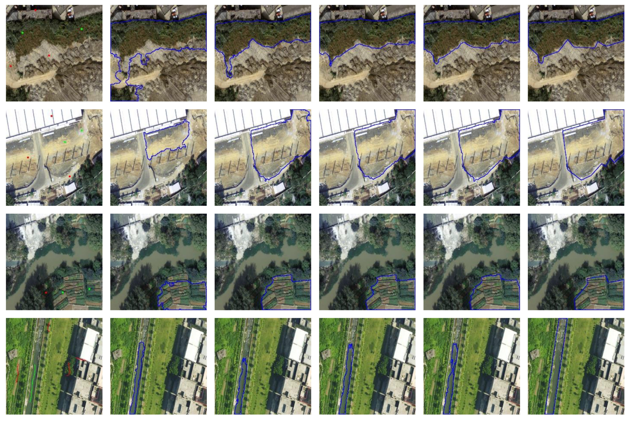
3. Experimental Results

To assess the effectiveness and generality of the proposed method, we conducted experiments on two datasets of high-resolution remote sensing images. Then, we described some implementation details in our work. Different from automatic segmentation task, we not only need to correctly segment the selected object, but also take user effort into consideration. Therefore, several evaluation indexes are used to assess the performance of the presented method in different scenes. Subsequently, we compared the experimental results of related works with ours. In addition, we further completed an ablation study to access the effectiveness of the proposed interaction transformation (PIT) and the proposed AGC module.

3.1. Dataset

Both datasets are used for high-resolution aerial imagery land cover classification tasks.

Table 1. Simple description of the two datasets.

Dataset	Size	GSD	Images	Location
Dataset 1	$4500\times 4500$	0.5m	60	None
Dataset 2	$3400\times 2800$	0.5m	12	China

presents their basic information. Dataset 1, annotated manually by our team, which was published in [45], is created for a pixel-wise classification task on real and complex engineered scenes. It contains 11 classes: background, farmland, garden, woodland, grassland, building, road, structures, pile, desert, and waters. We arranged the annotation into five categories: background, water, woodland, farmland, and bare land, for non-artificial region object extraction. Dataset 2 consists of two classes, namely, background and water, which is collected from the Chinese Geographic Condition Survey and Mapping Project. Given that models based on CNNs must be trained from fixed-size images, we cropped the images into $512\times 512$ pixels. Finally, 48,622 and 13,539 patches in training and test sets, respectively, are obtained from Dataset 1, and the training and test sets in Dataset 2 consisted of 6441 and 3278 patches. Figure 9 gives some examples of the training data from Dataset 1 and Dataset 2.

3.2. Implementation Details

We used the prevalent deep learning framework TensorFlow to implement the presented method. All experiments were conducted on a single 2080 GPU with 8 GB memory on board. The feature extraction model for the generation of feature maps F was pre-trained on the ImageNet dataset. We set the initial learning rate and weight decay as 0.001 and 0.0001, respectively, and the model using the Adam optimizer was trained for 100 epochs.

Because our method is more like an instance segmentation approach, we need to take some preprocessing operations to generate training data in our proposed rules from the standard semantic segmentation ground truth. First, for Dataset 1, we arranged the annotation into five categories: background, water, woodland, farmland, and bare land, for non-artificial region object extraction. As for Dataset 2, there is no need to do such an operation. After we obtained the one-class binary mask, we isolated each object instance to keep the connectivity in a $4\times 4$ neighborhood. Given that the one-class binary mask generated by our method has many discrete and broken objects, we deleted the tiny objects within $10\times 10$ pixels. In Section 2.1, we introduced our algorithm for the generation of guidance maps. For some parameter settings, we set the values of $N_{pos}^c$, $N_{neg}^{c1}$, $N_{neg}^{c2}$, $N_{pos}^s,$ and $N_{neg}^s$ to 10, 5, 5, 1, and 10, respectively. It is worth noting that we set these values as the maximum for the random sampling instead of fixing the number of random sampling. This strategy helps the random sampling simulate the process of user-provided interactions better.

3.3. Evaluation Indexes

To compare different methods quantitatively, we assessed the segmentation results in three different ways. First, for a single object, all the interactions sampled automatically from a ground truth mask were delivered to our segmentation network at once. Since there was nothing different from the standard semantic segmentation task, we adopted the common evaluation indexes, including intersection on union (IoU), precision, recall, and F1 score. They can be calculated as follows:

$$IoU=\frac{TP}{FN+TP+FP}$$

(14)

$$precision=\frac{TP}{TP+FP}$$

(15)

$$recall=\frac{TP}{TP+FN}$$

(16)

$$F1=2\times \frac{precision\times recall}{precision+recall}$$

(17)

where $TP$ denotes the positive pixels that we truly predicted, $FN$ and $FP$ present the positive and negative pixels that we falsely predicted, respectively.

Second, we followed the evaluation index in [25], specially used to evaluate the interactive segmentation method. Because the proposed strategy for training cannot correct errors created during the prediction process, we simulated the progressive interaction process by random sampling from the errors. Then, we counted the average number of interactions (clicks or scribbles both available) required to reach a certain (85%) IoU or until interactions were sampled 20 times. Third, considering that the proposed method was based on interactions between a human and computer, we evaluated the performance using the same index as the second evaluation method, with real human input.

3.4. Comparison with Related Works

The proposed method was compared with other state-of-the-art interactive segmentation approaches: Graph cut [46], DIOS [25], and LD [28]. We compared with other models that used the same settings (learning rate, weight decay, and training epoch are set as 0.001, 0.0001, and 100, respectively, except for the traditional algorithm Graph cut [46]) as our work to obtain a fair comparison. The detailed results using the first evaluation method are reported in

Table 2. Quantitative comparison with related methods on Dataset 1.

Method	IoU	Precision	Recall	F1
Graph cut [46]	66.52%	79.47%	81.59%	76.54%
DIOS [25]	73.67%	76.65%	93.63%	84.25%
LD [28]	76.07%	78.96%	95.80%	85.79%
AGMSSeg-Net	81.09%	83.81%	96.03%	88.62%

and

Table 3. Quantitative comparison with related methods on Dataset 2.

Method	IoU	Precision	Recall	F1
Graph cut [46]	75.22%	86.40%	84.15%	85.23%
DIOS [25]	78.27%	88.24%	82.94%	86.42%
LD [28]	81.29%	83.46%	97.27%	89.11%
AGMSSeg-Net	85.87%	94.79%	90.51%	91.98%

. Figure 10 intuitively shows some corresponding extraction results with different methods. Positive and negative samplings are displayed in green and red, respectively, and selected object boundaries are outlined in blue.

For this part, we do not take progressive interactions into account, just to see how the integration of interactions affects the extraction result. As we can see, our approach can extract complex objects with uncertain boundaries (the first three rows), and can generate more accurate boundaries of objects (the last three rows). Given that most of the non-artificial region objects are irregular in size and shape, it is hard for algorithms to extract the accurate boundaries from equivocal appearances. For instance, in the first row of Figure 10, the boundary of the woodland is completely irregular, which makes it difficult to distinguish between the woodland and bare land at the intersection. By taking the attention mechanism and multi-scale strategy into consideration, our method can focus on the selected location to extract a smoother and more accurate boundary, as shown in the fifth column. In the last row of Figure 10, there is a small patch of bare land (something like a dock) near the selected pond, which is sampled with a negative red click point. The proposed AGMSSeg-Net extracts the accurate boundary of the selected pond while other methods cannot get rid of the interference from the small patch. Specific channels and locations can provide more useful and important information to extract specific objects. We can use this algorithm to guide the network to segment objects.

To evaluate user effort in the process of interaction, we used the second evaluation method.

Table 4. Average number of interactions required to reach 85% IoU on Dataset 1 and Dataset 2.

Method	Dataset 1	Dataset 2
DIOS [25]	11.31	10.34
LD [28]	8.79	8.02
AGMSSeg-Net	7.32	6.57

shows that the presented method achieves better performance in both datasets. Lower is better, which means less effort is required to refine the segmentation result to reach 85% IoU. For instance, 6.57 interactions are required to segment the object with our presented method, while 8.02 interactions are needed with LD [28] on Dataset 2. Different from the existing methods, our algorithm both support interactions based on clicks and scribbles, which means we can choose the best way of sampling according to the real scenes. The average number of interactions required to reach a certain IoU is effectively reduced by adopting this strategy. In addition, the existing methods are designed to annotate the natural objects in the standard datasets, such as Semantic Boundaries Dataset, Pascal VOC Dataset, MS COCO Dataset, etc. However, the high-resolution satellite images are totally different from images in the natural datasets above. There may be very large variations of the objects in terms of their size, texture, shape, and contextual complexity in the image. The proposed AGMSSeg-Net helps promote performance by generating more accurate binary masks.

In addition, we also evaluated our method with real human input. Fifty non-artificial region object extraction tasks (50 images selected randomly from the test sets of the two datasets, called Subset 1) were given to three volunteers, to reach 85% IoU or until they were sampled 20 times. The order of the methods is not given, and volunteers do not see the current performance except for the IoU of the extracted result. We also counted the average time of each extraction process.

Table 5. Average number of interactions and time required to reach 85% IoU with human input.

Method	Subset 1	Time(ms)
DIOS [25]	8.69	532
LD [28]	6.45	257
AGMSSeg-Net	5.76	479

reports the performance of different methods on this set of images. As the table shows, our method achieves better results without significantly increasing the computation time. Therefore, our approach can be adapted efficiently to practical applications.

3.5. Ablation Study

To analyze the effectiveness of the proposed interaction transformation (PIT), the pre-trained feature maps (PFM), and the AGC module, we conducted the ablation experiments on Dataset 1 and Dataset 2. We set the learning rate, weight decay, and training epoch as 0.001, 0.0001, and 100, respectively.

Table 6. Ablation experiments of the methods without different modules.

Method	Dataset 1	Dataset 2
Without PIT	76.93	78.63
Without PFM	78.74	80.06
Without AGC	79.94	83.32
AGMSSeg-Net	81.09	85.87

shows the corresponding performance (presented by the evaluation index of IoU).

3.5.1. Without the Proposed Interaction Transformation

Different from the prevalent interactive segmentation methods, our approach adopted several transformations, such as EDT, GDT, and binary sampling transformation. More rich information can be collected by our strategy. The result in Table 6 shows that the proposed interaction transformation (PIT) improves the performance by 4.16% on Dataset 1 and 7.24% on Dataset 2. As shown in Figure 11, the PIT helps extract the boundary with higher completeness, and adapt to various objects in terms of size, texture, and shape.

3.5.2. Without the Pre-Trained Feature Maps

In [25], the model only adopted two Euclidean distance maps as the guidance maps, which were concatenated with the raw image as the input of standard FCN [18]. However, LD [28] not only adopted the interaction encoding maps but also concatenated the pre-trained feature maps to the raw input image. In addition, [28] used the dimensional reduction operation on the input data to select the feature tensors. Inspired by [28], we also used this strategy to include our input data for the task of interactive extraction. To figure out if the pre-trained feature maps are useful and the dimensional reduction operation is necessary, we conducted the ablation experiments on Dataset 1 and Dataset 2. The result in Table 6 shows that the pre-trained feature maps (PFM) improve the performance by 2.35% on Dataset 1 and 5.81% on Dataset 2. As shown in Figure 11, the PFM helps the LD [28] and AGMSSeg-Net extract more accurate boundaries than DIOS [25].

3.5.3. Without the AGC Module

Given that the multi-scale segmentation combined the cascade module and parallel module to cover objects in different sizes, our AGMSSeg-Net embedded the AGC module to focus on the specific channels and locations. Interactive extraction is based on the sampling provided by the users, which means all the information is not equal. The AGC module is quite suitable for this mechanism. From the performance of IoU presented in Table 6, we can see that the AGC module improves the performance by 1.15% on Dataset 1 and 2.55% on Dataset 2. As shown in Figure 11, specific channels and locations can provide more useful and important information to extract the selected objects.

4. Discussion

4.1. Interactions Transformation

For interaction transformation, our method mainly involves the following strategies: the relevance map modified by combining the positive and negative Euclidean distance maps, the ordinary interaction map based on the set of user-provided pixels, and the geodesic distance map using the geodesic distance transform. However, these strategies only use the pixel-level information. We can take the object-level information [34] into consideration. Since the inherent image structure plays an important role in image interpretation, we could transform interactions based on object-level to get hierarchical information.

4.2. Comparison with Existing Networks

U-Net, SegNet, and DeepLab [17,20,21] are prevalent networks for standard semantic segmentation task. These networks are fed with RGB-Channel input and extract robust feature tensors from the large datasets. A large number of experiments prove that these extracted features are suitable for segmentation tasks. However, interactive extraction not only uses RGB-Channel input but also receives user-interactions. These user-interactions are always present with encoding maps (such as Euclidean distance map), which are used as additional channels for segmentation. Standard semantic segmentation networks cannot meet the needs of interactive extraction without any modifications for additional channels.

DIOS [25] is the first work to use deep learning to solve interactive segmentation task in the domain of computer vision. In [25], user-provided clicks were transformed into a positive and a negative Euclidean distance maps, respectively, which were then concatenated with the raw image as the input of standard FCN [18]. It achieves very good results on simple and distinguishable scenes in natural images. However, equally treating the huge feature data is not a correct way to extracting non-artificial objects in complex satellite images. If such huge feature data are directly converted into the tensors used in the network without processing, the selected information will be compressed.

LD [28] presented a selection network to sort the segmentation results conforming to the user’s interactions. It provides an interesting idea to select the segmentation results and improves the effect of diversity in multiple semantic natural images. However, it just focuses on the diversity of objects by using a standard CAN [38] network. Without taking the size and shape of the non-artificial objects into account, it will miss scale information in the satellite images. In addition, keeping the feature maps at the original resolution in [28] costs huge computation resources.

The proposed AGMSSeg-Net can solve these problems with several special operations. Given that there are so many additional channels embedded in the raw input image, we adopted a dimensional reduction processing after concatenating all the input maps. This strategy reduces the computation resources and makes the input data suitable for segmentation network. Besides, our model combines user-provided interactions and robust feature maps extracted with powerful CNNs more efficiently. To overcome the selected information compression, we adopted the AGC module to reweight the feature tensors. Learning more suitable and scientific weights helps to make full use of the user-interactions and filter out interference information. Since there are very large variations of the objects in terms of their size, texture, shape, and contextual complexity, we took the scale viability problem into account and combined the cascade module with the parallel module by uniting the output tensors from each step stacked with an AGC module. All the proposed modules consider the particularities of the interactive extraction task and the complexity of satellite images.

The results of the proposed segmentation network are effective for non-artificial region object extraction from complex scenes in high-resolution satellite images. There are several advantages compared to other interactive segmentation methods. For instance, by combining the cascade module and parallel module, our multi-scale segmentation focuses on the specific locations to cover objects in terms of various sizes. As shown in Figure 12, we segmented the water body instance one by one. As we can see, the proposed AGMSSeg-Net not only accurately segments the big-scale river, but also segments the small-scale pond. Even if they are very close to each other, the results preserve the true shapes of each object instance.

There are also some limitations that must be overcome. The segmentation method is based on deep learning, which is limited to the quality of the image that we can provide. When the object is mixed up with different types, it is hard for the model to distinguish which part is the target that we select. As shown in Figure 13, the farmland is surrounded by woodland and other objects, and there are several trees in the selected farmland. The model cannot figure out the type of the object according to the mixed features and result in poor performance.

4.3. Difference between Artificial and Non-Artificial Objects

In fact, our method presented in this paper is used for the interactive extraction of non-artificial region objects from high-resolution satellite imagery, which refers to woodland, bare land, farmland, and water. The artificial objects (such as building, road, structure, and so on) are hugely influenced by human activities, which have enormous within-cluster variations in real challenging scenes. It is worth noting that we did not evaluate our method on artificial objects because we think there should be more special operations to obtain good results for this challenging task.

4.4. Human-in-the-Loop

In practical application, our method presented in this paper extracts region objects one by one, which disregards the relationships between the former and the latter extraction. It is unreasonable that the user’s effort would not decrease the next time when they have encountered the same problem as before. Interactive extraction should be a progressive learning process. In the process of user interactions and corrections of the results, the system needs to continuously conduct increment learning to generate a new model. The new model completes the extraction of the selected object, and then receives the correction provided by the user to update itself, and so on. We call this mechanism “Human-in-the-Loop”. It is something like the Relevance Feedback System [47], which iteratively receives corrections from the system and uses it to learn a better system. The model will become more and more intelligent, and the user effort will become less and less in the incremental learning process. Finally, the purpose of improving the work efficiency of interactive imagery interpretation will be achieved.

5. Conclusions

In this paper, we propose an interactive non-artificial region object extraction approach based on an attention-guided multi-scale segmentation network. A simple yet effective strategy to simulate user interactions by random sampling clicks and scribbles based on some rules is presented. Then, the interaction information is transformed into guidance maps composed of a relevance map, two geodesic distance maps, and a sampling map. We can make full use of the user-provided interactions by combining these guidance maps with the input image. To extract rich features from the input image, we apply a VGG network pre-trained on the ImageNet dataset to obtain multi-layer feature maps. After concatenating the image, the guidance maps and feature maps as input tensors, we feed them into the multi-scale segmentation network to generate a binary mask. In addition, a novel Attention-Guided Convolution module is embedded into the segmentation network to obtain a more accurate result. Finally, a post-processing method based on fully connected CRF is adapted to the segmentation mask, to extract the selected object boundary. Abundant experiments demonstrate that the presented approach is effective and robust for the interactive extraction of non-artificial region objects from high-resolution satellite images.

In future works, we will focus on the following areas: a more reasonable interaction transformation for making full use of user-provided information, a more robust segmentation network for obtaining the accurate binary mask, a more suitable model for both the interactive extraction of artificial and non-artificial objects and a new mechanism for using the relationships among the successively selected object, to promote the performance of the proposed method and improve work efficiency.

References

1. Mobley, C.D.; Sundman, L.K.; Davis, C.O.; Bowles, J.H.; Gleason, A. Interpretation of hyperspectral remote-sensing imagery by spectrum matching and look-up tables. Appl. Opt. 2005, 44, 3576–3592. [Google Scholar] [CrossRef]
2. Walter, V.; Luo, F. Automatic interpretation of digital maps. ISPRS J. Photogramm. Remote Sens. 2011, 4, 519–528. [Google Scholar] [CrossRef]
3. Tan, Y.; Yu, Y.; Xiong, S.; Tian, J. Semi-Automatic Building Extraction from Very High Resolution Remote Sensing Imagery Via Energy Minimization Model. In Proceedings of the IEEE International Geoscience and Remote Sensing Symposium (IGARSS), Beijing, China, 10–15 July 2016; pp. 657–660. [Google Scholar]
4. Zhang, C.; Yu, Z.; Hu, Y. A method of Interactively Extracting Region Objects from high-resolution remote sensing image based on full connection CRF. In Proceedings of the 10th IAPR Workshop on Pattern Recognition in Remote Sensing (PRRS), Beijing, China, 19–20 August 2018; pp. 1–6. [Google Scholar]
5. Fazan, A.J.; Dal, P.; Aluir, P. Rectilinear building roof contour extraction based on snakes and dynamic programming. Int. J. Appl. Earth Obs. Geoinf. 2013, 25, 1–10. [Google Scholar] [CrossRef]
6. Osman, J.; Inglada, J.; Christophe, E. Interactive object segmentation in high resolution satellite images. In Proceedings of the 2009 IEEE International Geoscience and Remote Sensing Symposium, Cape Town, South Africa, 12–17 July 2009; Volume 5, pp. 48–51. [Google Scholar]
7. Krizhevsky, A.; Sutskever, I.; Hinton, G.E. ImageNet classification with deep convolutional neural networks. Adv. Neural Inf. Process. Syst. 2012, 25, 1097–1105. [Google Scholar] [CrossRef]
8. Szegedy, C.; Liu, W.; Jia, Y.; Sermanet, P.; Reed, S.; Anguelov, D.; Erhan, D.; Vanhoucke, V.; Rabinovich, A. Going deeper with convolutions. In Proceedings of the IEEE Conference on Computer Vision and Pattern Recognition (CVPR), Boston, MA, USA, 7–12 June 2015; pp. 1–9. [Google Scholar]
9. Simonyan, K.; Zisserman, A. Very deep convolutional networks for large-scale image recognition. arXiv 2014, arXiv:1409.1556. [Google Scholar]
10. He, K.; Zhang, X.; Ren, S.; Sun, J. Deep residual learning for image recognition. In Proceedings of the IEEE Conference on Computer Vision and Pattern Recognition (CVPR), Las Vegas, NV, USA, 27–30 June 2016; pp. 770–778. [Google Scholar]
11. Girshick, R.; Donahue, J.; Darrell, T.; Malik, J. Rich feature hierarchies for accurate object detection and semantic segmentation. In Proceedings of the IEEE Conference on Computer Vision and Pattern Recognition (CVPR), Washington, DC, USA, 23–28 June 2014; pp. 580–587. [Google Scholar]
12. Girshick, R. Fast R-CNN. In Proceedings of the International Conference on Computer Vision (ICCV), Santiago, Chile, 13–16 December 2015; pp. 1440–1448. [Google Scholar]
13. Ren, S.; He, K.; Girshick, R.; Sun, J. Faster R-CNN: Towards Real-Time Object Detection with Region Proposal Networks. IEEE Trans. Pattern Anal. Mach. Intell. 2016, 39, 1137–1149. [Google Scholar] [CrossRef] [Green Version]
14. He, K.; Gkioxari, G.; Dollár, P.; Girshick, R. Mask R-CNN. In Proceedings of the IEEE International Conference on Computer Vision (ICCV), Venice, Italy, 22–29 October 2017; pp. 2980–2988. [Google Scholar]
15. Redmon, J.; Divvala, S.; Girshick, R.; Farhadi, A. You Only Look Once: Unified, Real-Time Object Detection. In Proceedings of the IEEE Conference on Computer Vision and Pattern Recognition (CVPR), Las Vegas, NV, USA, 27–30 June 2015; pp. 779–788. [Google Scholar]
16. Liu, W.; Anguelov, D.; Erhan, D.; Szegedy, C.; Reed, S.; Fu, C.Y.; Berg, A.C. SSD: Single shot multibox detector. In Proceedings of the European Conference on Computer Vision (ECCV), Amsterdam, The Netherlands, 11–14 October 2016; pp. 21–37. [Google Scholar]
17. Ronneberger, O.; Fischer, P.; Brox, T. U-Net: Convolutional Networks for Biomedical Image Segmentation. In Proceedings of the International Conference on Medical Image Computing and Computer-Assisted Intervention, Boston, MA, USA, 14–18 September 2015; pp. 234–241. [Google Scholar]
18. Long, J.; Shelhamer, E.; Darrell, T. Fully convolutional networks for semantic segmentation. In Proceedings of the IEEE Conference on Computer Vision and Pattern Recognition (CVPR), Boston, MA, USA, 7–12 June 2015; pp. 3431–3440. [Google Scholar]
19. Zhao, H.; Shi, J.; Qi, X.; Wang, X.; Jia, J. Pyramid Scene Parsing Network. In Proceedings of the IEEE Conference on Computer Vision and Pattern Recognition (CVPR), Honolulu, HI, USA, 21–26 July 2017; pp. 2881–2890. [Google Scholar]
20. Badrinarayanan, V.; Kendall, A.; Cipoll, R. Segnet: A deep convolutional encoder-decoder architecture for image segmentation. IEEE Trans. Pattern Anal. Mach. Intell. 2017, 39, 2481–2495. [Google Scholar] [CrossRef] [PubMed]
21. Chen, L.C.; Papandreou, G.; Kokkinos, I.; Murphy, K.; Yuille, A.L. DeepLab: Semantic Image Segmentation with Deep Convolutional Nets, Atrous Convolution, and Fully Connected CRFs. IEEE Trans. Pattern Anal. Mach. Intell. 2018, 40, 834–848. [Google Scholar] [CrossRef] [PubMed]
22. Saito, S.; Yamashita, T.; Aoki, Y. Multiple Object Extraction from Aerial Imagery with Convolutional Neural Networks. J. Imaging Sci. Technol. 2016, 60, 1–9. [Google Scholar] [CrossRef]
23. Kussul, N.; Lavreniuk, M.; Skakun, S.; Shelestov, A. Deep Learning Classification of Land Cover and Crop Types Using Remote Sensing Data. IEEE Geosci. Remote Sens. Lett. 2017, 14, 778–782. [Google Scholar] [CrossRef]
24. Kemker, R.; Salvaggio, C.; Kanan, C. Algorithms for semantic segmentation of multispectral remote sensing imagery using deep learning. ISPRS J. Photogramm. Remote Sens. 2018, 145, 60–77. [Google Scholar] [CrossRef] [Green Version]
25. Xu, N.; Price, B.; Cohen, S.; Yang, J.; Huang, T. Deep Interactive Object Selection. In Proceedings of the IEEE Conference on Computer Vision and Pattern Recognition (CVPR), Las Vegas, NV, USA, 26 June–1 July 2016; pp. 373–381. [Google Scholar]
26. Rajchl, M.; Lee, M.; Oktay, O.; Kamnitsas, K.; Passerat-Palmbach, J.; Bai, W.; Rutherford, M.; Hajnal, J.; Kainz, B.; Rueckert, D. DeepCut: Object Segmentation from Bounding Box Annotations using Convolutional Neural Networks. IEEE Trans. Med. Imaging 2016, 36, 674–683. [Google Scholar] [CrossRef] [PubMed] [Green Version]
27. Wang, G.; Zuluaga, M.A.; Li, W.; Pratt, R.; Patel, P.A.; Aertsen, M.; Doel, T.; David, A.L.; Deprest, J.; Ourselin, S.; et al. DeepIGeoS: A Deep Interactive Geodesic Framework for Medical Image Segmentation. IEEE Trans. Pattern Anal. Mach. Intell. 2017, 41, 1559–1572. [Google Scholar] [CrossRef] [PubMed]
28. Li, Z.; Chen, Q.; Koltun, V. Interactive image segmentation with latent diversity. In Proceedings of the IEEE Conference on Computer Vision and Pattern Recognition (CVPR), Salt Lake City, UT, USA, 18–22 June 2018; pp. 577–585. [Google Scholar]
29. Wu, W.; Qi, H.; Rong, Z.; Rong, Z.; Liu, L.; Su, H. Scribble-Supervised Segmentation of Aerial Building Footprints Using Adversarial Learning. IEEE Access 2018, 6, 58898–58911. [Google Scholar] [CrossRef]
30. Song, X.; He, G.; Zhang, Z.; Long, T.; Peng, Y.; Wang, Z. Visual attention model based mining area recognition on massive high-resolution remote sensing images. Clust. Comput. 2015, 2, 541–548. [Google Scholar] [CrossRef]
31. Shakeel, A.; Sultani, W.; Ali, M. Deep built-structure counting in satellite imagery using attention based re-weighting. ISPRS J. Photogramm. Remote Sens. 2019, 151, 313–321. [Google Scholar] [CrossRef] [Green Version]
32. Xu, R.; Tao, Y.; Lu, Z.; Zhong, Z. Attention-mechanism-containing neural networks for high-resolution remote sensing image classification. Remote Sens. 2018, 10, 1602. [Google Scholar] [CrossRef] [Green Version]
33. Maninis, K.K.; Caelles, S.; Pont-Tuset, J.; Luc, V.G. Deep extreme cut: From extreme points to object segmentation. In Proceedings of the IEEE Conference on Computer Vision and Pattern Recognition (CVPR), Salt Lake City, UT, USA, 18–22 June 2018; pp. 616–625. [Google Scholar]
34. Majumder, S.; Yao, A. Content-Aware Multi-Level Guidance for Interactive Instance Segmentation. In Proceedings of the IEEE Conference on Computer Vision and Pattern Recognition (CVPR), Long Beach, CA, USA, 16–20 June 2019; pp. 11602–11611. [Google Scholar]
35. Ling, H.; Gao, J.; Kar, A.; Chen, W.; Fidler, S. Fast interactive object annotation with curve-gcn. In Proceedings of the IEEE Conference on Computer Vision and Pattern Recognition (CVPR), Long Beach, CA, USA, 16–20 June 2019; pp. 5257–5266. [Google Scholar]
36. Lee, T.C.; Kashyap, R.L.; Chu, C.N. Building skeleton models via 3-D medial surface axis thinning algorithms. Graph. Models Image Process. 1994, 56, 462–478. [Google Scholar] [CrossRef]
37. Criminisi, A.; Sharp, T.; Blake, A. GeoS: Geodesic image segmentation. In Proceedings of the European Conference on Computer Vision (ECCV), Marseille, France, 11–14 October 2008; Springer: Berlin/Heidelberg, Germany, 2018; pp. 99–112. [Google Scholar]
38. Fisher, Y.; Vladlen, K. Multi-Scale Context Aggregation by Dilated Convolutions. arXiv 2015, arXiv:1511.07122. [Google Scholar]
39. Chen, L.C.; Papandreou, G.; Schroff, F.; Adam, H. Rethinking Atrous Convolution for Semantic Image Segmentation. arXiv 2017, arXiv:1706.05587. [Google Scholar]
40. Wang, F.; Jiang, M.; Qian, C.; Yang, S.; Li, C.; Zhang, H.; Wang, X.; Tang, X. Residual Attention Network for Image Classification. In Proceedings of the IEEE Conference on Computer Vision and Pattern Recognition (CVPR), Honolulu, HI, USA, 21–26 July 2017; pp. 3156–3164. [Google Scholar]
41. Jie, H.; Li, S.; Albanie, S.; Sun, G.; Wu, E. Squeeze-and-Excitation Networks. In Proceedings of the IEEE Conference on Computer Vision and Pattern Recognition (CVPR), Salt Lake City, UT, USA, 18–22 June 2018; pp. 7132–7141. [Google Scholar]
42. Fu, J.; Zheng, H.; Mei, T. Look Closer to See Better: Recurrent Attention Convolutional Neural Network for Fine-grained Image Recognition. In Proceedings of the IEEE Conference on Computer Vision and Pattern Recognition (CVPR), Honolulu, HI, USA, 21–26 July 2017; pp. 4438–4446. [Google Scholar]
43. Goodfellow, I.; Bengio, Y.; Courcille, A. Deep Learning; MIT Press: Cambridge, MA, USA, 2016. [Google Scholar]
44. Krähenbühl, P.; Koltun, V. Efficient Inference in Fully Connected CRFs with Gaussian Edge Potentials. arXiv 2012, arXiv:1210.5644. [Google Scholar]
45. Zhang, M.; Hu, X.; Zhao, L.; Lv, Y.; Luo, M.; Pang, S. Learning dual multi-scale manifold ranking for semantic segmentation of high-resolution images. Remote Sens. 2017, 9, 500. [Google Scholar] [CrossRef] [Green Version]
46. Boykov, Y.; Veksler, O.; Zabih, R. Fast approximate energy minimization via graph cuts. IEEE Trans. Pattern Anal. Mach. Intell. 2001, 23, 1222–1239. [Google Scholar] [CrossRef] [Green Version]
47. Zhou, X.; Huang, T. Relevance feedback in image retrieval: A comprehensive review. Multimed. Syst. 2003, 8, 536–544. [Google Scholar] [CrossRef]
Figure 1. Flowchart of the proposed non-artificial region object extraction method. The Attention-Guided Convolution (AGC) enhanced multi-scale segmentation network is described in detail in Section 2.2.
Remotesensing 12 00789 g001
Figure 2. We apply different sampling strategies (green for positive sampling and red for negative sampling) to cover various region objects that are irregular in size and shape. (a) Click sampling for a pond and (b) scribble sampling for a river.
Remotesensing 12 00789 g002
Figure 3. Results of scribble generation for non-artificial region objects from satellite images. (a) Original image, (b) ground truth mask, (c) positive scribble mask, and (d) negative scribble mask. The four rows of images represent “bare land”, “farmland”, “water”, and “woodland”, respectively.
Remotesensing 12 00789 g003
Figure 4. A comparison of different methods for interaction transformation. (a) Input image with clicks or scribbles sampling (green for positive sampling and red for negative sampling), (b) sampling map, (c) Euclidean distance transformation (EDT) map for positive sampling, (d) Geodesic distance transformation (GDT) map for positive sampling, and (e) relevance map.
Remotesensing 12 00789 g004
Figure 5. Structure of the Attention-Guided Convolution module. The dimensions of the blue tensors are 64 at the size of 128 × 128 . The convolution with 1 × 1 kernel was used in this module, and the value of C is set as 64 in the proposed work.
Remotesensing 12 00789 g005
Figure 6. Intuitive description of the difference among 3 × 3 convolution kernel with 1, 2, and 3 dilation rates. The red pixel in the image represents the original point of the 3 × 3 convolution kernel. (a) Receptive field of 3 × 3 with 1-dilated convolution, (b) receptive field of 5 × 5 with 2-dilated convolution, and (c) receptive field of 7 × 7 with 3-dilated convolution.
Remotesensing 12 00789 g006
Figure 7. Attention-guided multi-scale segmentation network structure. The dimensions of the blue tensors are 64 at the size of 128 × 128 .
Remotesensing 12 00789 g007
Figure 8. Post-processing with fully connected Conditional Random Field (CRF). (a) The input images, (b) the segmentation masks, and (c) the final object extraction results. We obtained the boundary of the selected object from our segmentation mask, which was outlined by a blue closed curve.
Remotesensing 12 00789 g008
Figure 9. Examples of the training sample from Dataset 1 (first two columns) and Dataset 2 (last two columns). (a,c) The RGB images and (b,d) the corresponding label images (Dataset 1 consists of 11 classes, Dataset 2 only supports binary mask, white for water, and black for background).
Remotesensing 12 00789 g009aRemotesensing 12 00789 g009b
Figure 10. Some corresponding visual results of different methods. The first four rows of images (representing “woodland”, “bare land”, “farmland” and “water”, respectively) are from Dataset 1, and the others are from Dataset 2. Input images with (a) interactions, (b) Graph cut [46], (c) DIOS [25], (d) LD [28], (e) AGMSSeg-Net, and (f) ground truth.
Remotesensing 12 00789 g010aRemotesensing 12 00789 g010b
Figure 11. Some visual results compared with AGMSSeg-Net. The four rows of images represent “woodland”, “bare land”, “farmland”, and “water”, respectively. (a) Input image, (b) result without proposed interaction transformation (PIT), (c) result without pre-trained feature maps (PFM), (d) result without AGC, (e) result with the AGMSSeg-Net, and (f) the ground truth.
Remotesensing 12 00789 g011
Figure 12. Some visual segmentation results of isolated object instances. The first row represents the ground truth, and the last row represents the corresponding segmentation result. (a) Input image and extraction result and (bg) isolated object instances.
Remotesensing 12 00789 g012
Figure 13. Some visual segmentation results. (a) Input image, (b) our result, and (c) the ground truth.
Remotesensing 12 00789 g013