Sketch-Based Subspace Clustering of Hyperspectral Images

Abstract

Sparse subspace clustering (SSC) techniques provide the state-of-the-art in clustering of hyperspectral images (HSIs). However, their computational complexity hinders their applicability to large-scale HSIs. In this paper, we propose a large-scale SSC-based method, which can effectively process large HSIs while also achieving improved clustering accuracy compared to the current SSC methods. We build our approach based on an emerging concept of sketched subspace clustering, which was to our knowledge not explored at all in hyperspectral imaging yet. Moreover, there are only scarce results on any large-scale SSC approaches for HSI. We show that a direct application of sketched SSC does not provide a satisfactory performance on HSIs but it does provide an excellent basis for an effective and elegant method that we build by extending this approach with a spatial prior and deriving the corresponding solver. In particular, a random matrix constructed by the Johnson-Lindenstrauss transform is first used to sketch the self-representation dictionary as a compact dictionary, which significantly reduces the number of sparse coefficients to be solved, thereby reducing the overall complexity. In order to alleviate the effect of noise and within-class spectral variations of HSIs, we employ a total variation constraint on the coefficient matrix, which accounts for the spatial dependencies among the neighbouring pixels. We derive an efficient solver for the resulting optimization problem, and we theoretically prove its convergence property under mild conditions. The experimental results on real HSIs show a notable improvement in comparison with the traditional SSC-based methods and the state-of-the-art methods for clustering of large-scale images.

1. Introduction

Hyperspectral images (HSIs), acquired by the hyperspectral cameras, record the spectrum of materials covering a wide range of wavelengths. The rich spectral information of HSIs enables discriminating the materials that are often visually indistinguishable, which led to a number of applications in remote sensing, such as target detection [1,2], environmental monitoring [3], geosciences, defense and security [4]. It is often desired to categorize pixels in the imaged scene into different classes, corresponding to different materials or different types of objects. When no training data is available, this task is called clustering. Hence, clustering is also referred to as unsupervised classification.

Two most popular clustering methods are fuzzy c-means (FCM) [5] and k-means [6,7] due to their simplicity and superior computational efficiency. They group data points by finding the minimum distance between test data and each cluster centroid which is updated iteratively. However, their performance is sensitive to initial conditions and noise.

Recently, spectral clustering-based methods [8,9,10,11,12,13] have achieved a great success and have been widely applied in various fields due to excellent performance and robustness to noise [14]. In general, these methods first define a similarity matrix to construct a graph of data points, which is learned from the input data under different critera. Then, the resulting similarity matrix is used within the spectral clustering framework. The performance of spectral clustering heavily depends on the similarity matrix [14], hence, its construction is a crucial step. Many of these methods, like local subspace affinity (LSA) [15], spectral local best-fit flats (SLBF) [16] and locally linear manifold clustering (LLMC) [17] build the similarity matrix with k nearest neighbours (KNN) using angle or Euclidean distance between two data points. This approach tends to treat erroneously the data points near the intersection of two subspaces because their closest points often lie in another subspace.

The recent sparse subspace clustering (SSC) method [11] constructs the similarity matrix based on the self-expressiveness model where the input data is employed as the representation dictionary. SSC models a high-dimensional data space as a union of low-dimensional subspaces. The key insight is that, for each data point in the subspace ${\mathcal{S}}_i$, the global solution of the sparse coding problem with the self-representation dictionary automatically selects the data points in the same subspace ${\mathcal{S}}_i$. Thus, each data point gets automatically represented as a sparse linear or affine combination of other points in the same subspace. This is called subspace preserving property and is explicitly expressed by non-zero entries of the coefficient matrix $\mathbf{C}$: i-th and j-th data points are in the same subspace if $C_{i,j}\ne 0$. The coefficient matrix leads directly to the similarity matrix for spectral clustering.

As the SSC model calculates sparse coefficients individually and independently for each input data point, the clustering performance is sensitive to noise. In order to solve this problem, various extensions have been proposed with the aim to encode the spatial dependencies among the neighbouring data points in hyperspectral data, and obtain thereby more accurate similarity matrices and improved clustering results [18,19,20,21,22,23,24,25]. Guo et al. [18,19] focus on the clustering of 1-D drill hole hyperspectral data and regularize the coefficients of neighbouring data points in depth to be similar by a ${\ell }_1$ norm based smoothing regularization. For the 2-D spatial-wise hyperspectral images, a smoothing strategy was introduced in Reference [20] by minimizing the difference between coefficients corresponding to the central pixel and to the mean of pixels in a local square window. A kernel version of SSC incorporating max pooling of the sparse coefficient matrix was presented in Reference [21]. The spectral-spatial SSC method of Reference [22] integrates an ${\ell }_2$ spatial regularizer with the SSC model (L2-SSC), to penalize abrupt differences between the coefficients of nearby pixels. In Reference [23,25], an ${\ell }_{1,2}$ norm constraint on the coefficients of pixels in each local region was incorporated in the SSC model. Based on the collaborative representation with an ${\ell }_2$ norm constraint on the coefficients, a novel model with a locally adaptive dictionary was proposed in Reference [24].

While showing excellent performances, the above mentioned methods are also of considerable computational complexity, resulting from iterative optimization. The time complexity in each iteration is typically in the range of $\mathcal{O}({\left(MN\right)}^3)$, where M and N are the number of rows and columns in each band. For large scale HSIs with millions of pixels in each band, this bound can thus exceed ${10}^{18}$ elementary operations per iteration, and such processing becomes often infeasible on the common computing platforms. The approaches reported in References [26,27] addressed this problem by constructing a graph based on a set of selected representative samples. In combination with modified spectral clustering methods, a lower complexity has been reached, but the clustering results are sensitive to the initially selected samples. Recently, some generalized large-scale methods [28,29,30] based on SSC have been proposed for clustering tasks in computer vision. In Reference [28], a scalable SSC method was designed for large-scale data sets, where a small part of samples are first randomly selected and clustered with the SSC model, and then clustering of remaining samples is executed by sparse coding with respect to the dictionary constructed from previously selected samples. The work in Reference [29] studied an efficient SSC model based on orthogonal matching pursuit (OMP) and discussed theoretical conditions for subspace preserving representation. A recent sketched SSC model of Reference [30] lowers the computational burden of SSC by using a clever random projection technique to sketch and compress the input data to a computationally affordable level. While these large-scale SSC-based methods demonstrated success in real applications with facial images, handwritten text and news corpus data, to the best of our knowledge none of them was applied before in the clustering of HSIs. Our experiments show that despite the scalability of these methods, their clustering performance in HSIs turns out to be poor. This can be attributed to the complex spatial structure of HSIs, spectral noise and spectral variability.

In view of this, we propose a sketched sparse subspace clustering method with total variation (TV) spatial regularization, termed Sketch-SSC-TV, which can handle large-scale HSIs while achieving a high level of clustering performance. A sketching matrix constructed by a random matrix is firstly employed to build a sketched dictionary, which is much smaller than the self-representation dictionary, resulting in a significant reduction of the number of coefficients to be solved. By incorporating the spatial constraint as the TV norm on the coefficient matrix, the proposed model greatly promotes the connectivity of neighbouring pixels and improves the piecewise smoothness of clustering maps. Furthermore, we propose an algorithm with theoretically guaranteed global convergence to solve the resulting optimization problem. By adopting the sketching matrix, the optimization complexity of the TV-related sub-problem reduces from $\mathcal{O}({\left(MN\right)}^2\log \left(MN\right))$ to $\mathcal{O}\left(MNn\log \right(MN\left)\right)$ ($n<<MN$), facilitating thus greatly the processing of large-scale data. The similarity matrix is constructed by applying KNN on the obtained coefficient matrix, and further employed within the spectral clustering method. Experiments conducted on four HSIs show superior clustering performance compared to both traditional SSC-based methods and the related large-scale clustering methods. The major contributions of the paper can be summarized as follows.

• The most important contribution of this paper is a new SSC-based framework, which can be applied on large-scale HSIs while achieving excellent clustering accuracy. To the best of our knowledge, this is the first time to address the large-scale clustering problem of HSIs based on the SSC model.
• Different from the traditional SSC-based methods which use all the input data as a dictionary, we adopt a compressed dictionary by using random projection technique to reduce the dictionary size, which effectively enables a scalable subspace clustering approach.
• To account for the spatial dependencies among the neighbouring pixels, we incorporate a powerful TV regularization in our model, leading to a more discriminative coefficient matrix. The resulting model proves to be more robust to spectral noise and spectral variability.
• We develop an efficient algorithm to solve the resulting optimization problem and prove its convergence property theoretically.

The rest of this paper is organized as follows. Section 2 briefly introduces the clustering of HSIs with the SSC model. Section 3 describes the proposed Sketch-SSC-TV model and the resulting optimization problem. Experimental results on real HSIs are presented in Section 4. Section 5 concludes the paper.

2. HSI Clustering with the SSC Model

Let a B-band HSI be denoted as $\mathbf{Y}\in {\mathbb{R}}^{B\times MN}$, where the i-th vector ${\mathbf{y}}_i\in {\mathbb{R}}^B$ represents the spectral signature of the i-th pixel in HSI and $MN$ is the total number of pixels. Sparse subspace clustering (SSC) partitions the high-dimensional data space into a union of lower dimensional subspaces. Concretely, it assumes that all high-dimensional data points ${\mathbf{y}}_i$’s, that is, spectral signatures of all the pixels from a given HSI $\mathbf{Y}$, are drawn from a union of subspaces, each of which corresponds to a particular class. The key idea is that among infinitely many possibilities to represent a data point ${\mathbf{y}}_i$ in terms of other points, a sparse representation will select a few points that belong to the same subspspace as ${\mathbf{y}}_i$. This is known as the subspace preserving property. Thus, SSC starts from a self-representation model where the input data matrix $\mathbf{Y}$ is employed as a dictionary: $\mathbf{Y}=\mathbf{YC}$ and infers the coefficient matrix $\mathbf{C}\in {\mathbb{R}}^{MN\times MN}$ by solving the sparse coding problem (requiring that $\mathbf{C}$ is sparse) and ensuring that the trivial solution where each sample would be simply represented by itself is excluded. The non-zero entries in $\mathbf{C}$ will then indicate directly which data points lie within the common subspaces. Formally, SSC solves the following optimization problem:

$$\begin{array}{c}\hfill \underset{\mathbf{C}}{argmin}{\parallel \mathbf{C}\parallel }_1+{\displaystyle \frac{\lambda }{2}}{\parallel \mathbf{Y}-\mathbf{YC}\parallel }_F^{2}s.t.\mathrm{diag}\left(\mathbf{C}\right)=\mathbf{0},{\mathbf{1}}^T\mathbf{C}={\mathbf{1}}^T,\end{array}$$

(1)

where ${\parallel \mathbf{C}\parallel }_1={\sum }_i{\sum }_j\left|C_{ij}\right|$; $\mathbf{1}$ is an all-one vector; $\mathrm{diag}\left(\mathbf{C}\right)$ is a diagonal matrix whose entries outside the main diagonal are zero and $\lambda$ is a parameter, which controls the balance between the data fidelity and the sparsity of the coefficient matrix. The constraint $\mathrm{diag}\left(\mathbf{C}\right)=\mathbf{0}$ is introduced to avoid the trivial solution of representing a sample by itself and the second constraint ${\mathbf{1}}^T\mathbf{C}={\mathbf{1}}^T$ ensures that each data point is an affine combination of other data points.

The problem in (1) can be solved by the ADMM algorithm [31], with the time complexity of $\mathcal{O}({\left(MN\right)}^{2}B+{\left(MN\right)}^3(I+1))$ where I is the number of iterations. The coefficient matrix $\mathbf{C}$ yields directly the dependence structure among the data points: a non-zero entry $C_{ij}$ indicates that the samples ${\mathbf{y}}_i$ and ${\mathbf{y}}_j$ are in the same class. Thus, it is reasonable to construct the similarity matrix $\mathbf{W}\in {\mathbb{R}}^{MN\times MN}$ as

$$\begin{array}{c}\hfill \mathbf{W}=\left|\mathbf{C}\right|+{\left|\mathbf{C}\right|}^T,\end{array}$$

(2)

where $\left|\mathbf{C}\right|$ takes the absolute values of $\mathbf{C}$. The symmetric structure of $\mathbf{W}$ ensures that each pair of samples are connected to each other if either side is selected to represent another, which results in a strengthened connection of the graph. The similarity matrix $\mathbf{W}$ is then used as an input to spectral clustering [32] to produce the clustering result. Specifically, the Laplacian matrix $\mathbf{L}\in {\mathbb{R}}^{MN\times MN}$ is first formed by

$$\begin{array}{c}\hfill \mathbf{L}:=\mathbf{D}-\mathbf{W}\end{array}$$

(3)

where $\mathbf{D}\in {\mathbb{R}}^{MN\times MN}$ is a diagonal matrix with $D_{ii}={\sum }_j{W}_{ij}$ [33]. Then the c eigenvectors ${\left\{{\mathbf{v}}_k\right\}}_{k=1}^c$ of $\mathbf{L}$ corresponding to the c smallest non-zero eigenvalues of $\mathbf{L}$ are calculated via singular-value decomposition (SVD). Finally, the clustering result is obtained by running k-means clustering on the $MN\times c$ matrix $\mathbf{V}=[{\mathbf{v}}_{\mathbf{1}},\dots ,{\mathbf{v}}_{\mathbf{c}}]$.

3. Sketch-SSC-TV Model for HSIs

In this section, we first introduce our new SSC-based model with TV regularization (SSC-TV), to effectively account for the spatial dependencies between the input data points. Next, we incorporate a random sketching technique into this model, leading to our unified Sketch-SSC-TV model for large-scale HSIs. Finally, we develop an efficient optimization algorithm for the resulting model based on ADMM.

3.1. The SSC-TV Model

HSIs not only record the spectrum of materials in the spectral domain but also capture the distribution of ground-objects in the spatial domain. As the distribution of ground materials typically shows some continuity, HSIs are composed of various nearly homogeneous regions made of pixels that belong to the same class with a very high probability [34,35,36,37,38,39,40]. For this reason, spectral signatures of pixels within small local regions are typically very similar. Conversely, the pixels belonging to different classes are more likely to occupy different spatial locations and exhibit significantly different spectral characteristics. HSI clustering assigns pixels into distinct groups according to the spectral similarities such that the pixels from the same group are more similar to each other than to those from other groups. Here, each cluster is viewed as a subspace. Thus, by conducting subspace clustering the pixels of HSIs in local homogeneous regions are likely to be grouped together in the same cluster. At the same time, the pixels showing significant spectral differences, which are typically also spatially separated, are assigned to different clusters. This way, subspace clustering results in a meaningful interpretation of the spatial content of HSIs. Thus, idealy, the subspaces in the spectral domain correspond to the cluster structure in the spatial domain. However, due to noise and spectral variability, the actual results of the subspace clustering model differ from the ideal cluster structure, and do not agree perfectly with the spatial content. Such sensitivity to noise and to spectral variability is inherent to all the methods that perform pixel-wise processing and thus also to the SSC model in (1), where sparse coefficients are calculated independently for each pixel. Random variations in the recorded spectral responses affect the solution of the sparse coding problem such that in the resulting sparse representation some data points may be represented by data points from different subspaces. This degrades the construction of the similarity matrix, thereby deteriorating spectral clustering performance. We aim to alleviate this problem by imposing a spatial constraint that makes the model less sensitive to random spectral variations of individual pixels.

To accommodate for the fact that pixels within a local homogeneous region are likely to belong to the same class, we require explicitly that sparse coefficients of nearby pixels likely to be mutually similar, that is, selecting similar sets of pixels in the subspace-sparse representation. Formally, this means that the coefficient matrix $\mathbf{C}$ exhibits certain local smoothness. Recall that pixels ${\mathbf{y}}_i$ and ${\mathbf{y}}_j$ are likely to belong to the same class if $C_{ij}\ne 0$. In reality, $C_{ij}$ is rarely exactly 0, but the larger $C_{ij}$, the more likely it is that ${\mathbf{y}}_i$ and ${\mathbf{y}}_j$ are from the same class. Ideally, ${\mathbf{y}}_i$ as an atom in the dictionary, only contributes to the representation of pixels in the same class. Since neighbouring pixels from a local region of the input image $\mathbf{Y}$ usually belong to the same class in the ideal case, all of them are likely to select the same atoms in the subspace representation. Hence, any row of $\mathbf{C}$, ${\mathbf{c}}^i=[C_{i1},C_{i2},\dots ,C_{iMN}]$, composed of the coefficients that correspond to an atom ${\mathbf{y}}_i$, will reflect some aspect of the spatial structure of HSI. In other words, the ideal coefficients should reflect the local smoothness and discontinuities that are present in the original HSI, as shown in Figure 1, where each ${\mathbf{c}}^i$ is reshaped to a $M\times N$ 2-D slice. This motivates us to introduce TV spatial regularization on sparse coefficients, which promotes effectively piece-wise smoothness while preserving sharp transitions among the distinct regions.

Let $\mathbf{x}\in {\mathbb{R}}^{MN}$ denote a vector of raster scanned pixel values from a grayscale image of size $M\times N$ and define the anisotropic TV norm (An alternative isotropic TV norm formulation is ${\parallel \mathbf{x}\parallel }_{TV}={\sum }_{i=1}^{MN}\sqrt{{[{({\mathbf{H}}_x\mathbf{x})}_i]}^2+{[{({\mathbf{H}}_y\mathbf{x})}_i]}^2}$ where ${(·)}_i$ is the i-th element of a vector) as

$$\begin{array}{c}\hfill {\parallel \mathbf{x}\parallel }_{TV}=\parallel {\mathbf{H}}_x{\mathbf{x}\parallel }_1+{\parallel {\mathbf{H}}_y\mathbf{x}\parallel }_1,\end{array}$$

(4)

where ${\mathbf{H}}_x$ and ${\mathbf{H}}_y$ are the forward finite-difference operators in the horizontal and vertical directions, respectively, with periodic boundary conditions.

For the 2-D matrix $\mathbf{Y}$ reshaped from a 3-D HSI $\mathcal{Y}\in {\mathbb{R}}^{M\times N\times B}$ in HSI, the corresponding TV norm is formulated as

$$\begin{array}{cc}\hfill {\parallel \mathbf{Y}\parallel }_{TV}& =\parallel {\mathbf{H}}_x{\mathbf{Y}}^T{\parallel }_1+{\parallel {\mathbf{H}}_y{\mathbf{Y}}^T\parallel }_1.\hfill \end{array}$$

(5)

Now we incorporate the spatial constraint into the SSC model. In particular, we impose the TV norm as defined above on the sparse coefficient matrix $\mathbf{C}$, and formulate our SSC-TV model as

$$\begin{array}{c}\hfill \underset{\mathbf{C}}{argmin}{\displaystyle \frac{1}{2}}{\parallel \mathbf{Y}-\mathbf{YC}\parallel }_F^2+{\lambda \parallel \mathbf{C}\parallel }_1+{\lambda }_{tv}{\parallel \mathbf{C}\parallel }_{TV}s.t.\mathrm{diag}\left(\mathbf{C}\right)=\mathbf{0},{\mathbf{1}}^T\mathbf{C}={\mathbf{1}}^T,\end{array}$$

(6)

where $\lambda$ and ${\lambda }_{tv}$ are two penalty parameters corresponding to sparsity and spatial constraint, respectively. Like with the standard SSC, the similarity matrix is obtained from $\mathbf{C}$ by applying (2), and fed into the spectral clustering. The TV norm imposed on $\mathbf{C}$ promotes the local smoothness of the resulting subspace-sparse representation, which encourages neighbouring pixels to select a common set of pixels from the same class. Since pixels belonging to the same class tend to be spatially clustered as well (within one or multiple local regions), this locally smooth coefficient structure will also lead to an improved agreement of the resulting spectral clustering with the underlying spatial structure.

3.2. The Sketch-SSC-TV Model for Large-Scale HSIs

The problem at this point is to solve the sparse coefficient matrix $\mathbf{C}$ from the cost function in (6). However, as the number of pixels in HSIs, $MN$, is typically very large, the matrix $\mathbf{C}\in {\mathbb{R}}^{MN\times MN}$ in (6) is huge. The optimization problem of the SSC-TV model actually cannot be efficiently solved in practice due to its prohibitively high computational complexity. The traditional SSC-based methods [11,20,21,22,23,41,42] also suffer from the same problem. One key obstacle is that they have to calculate and save the inverse of the entire large matrix $({\mathbf{Y}}^T\mathbf{Y}+\mu \mathbf{I})\in {\mathbb{R}}^{MN\times MN}$ in memory based on the ADMM algorithm, whose time complexity reaches $\mathcal{O}\left({\left(MN\right)}^3\right)$, which is infeasible for large-scale data sets. In addition, for the TV-regularized model in (6), the complexity to solve the subproblem with respect to the TV-norm is $\mathcal{O}\left({\left(MN\right)}^2\log \left(MN\right)\right)$, which further increases the computation burden. Despite the effectiveness of incorporating the TV-norm in the tasks such as HSI unmixing [43,44], superresolution [45] and denoising [46,47,48], the exploitation of TV-regularization in the SSC model is impractical, especially for large-scale HSIs. In the following parts, a sketched SSC (Sketch-SSC) [30] method designed for large-scale data sets will be introduced, and then our Sketch-SSC-TV model is present.

3.2.1. The Sketch-SSC Model

The recently proposed Sketch-SSC method [30], which was explored in the context of computer vision, employs a random projection matrix $\mathbf{R}\in {\mathbb{R}}^{MN\times n}$ to sketch the input data, compressing the self-representation dictionary $\mathbf{Y}$ in (1) to a compact one $\mathbf{D}\in {\mathbb{R}}^{B\times n}:=\mathbf{YR}$. The objective function of the Sketch-SSC with respect to the sparse coefficient matrix $\mathbf{A}\in {\mathbb{R}}^{n\times MN}$ can be formulated as

$$\begin{array}{c}\hfill \underset{\mathbf{A}}{argmin}{\parallel \mathbf{A}\parallel }_1+{\displaystyle \frac{\lambda }{2}}{\parallel \mathbf{Y}-\mathbf{DA}\parallel }_F^2.\end{array}$$

(7)

By using the random sketching matrix $\mathbf{R}$, the number of optimization variables in the sparse matrix is significantly reduced, making the Sketch-SSC model applicable to large-scale data sets. We illustrate this pictorially in Figure 2. After obtaining the sparse matrix $\mathbf{A}$, the similarity matrix $\mathbf{W}$ is built via the KNN graph of $\mathbf{A}$ for spectral clustering.

The random matrix $\mathbf{R}\in {\mathbb{R}}^{MN\times n}$ used here is known as Johnson-Lindenstrauss transform (JLT), which can compress $\mathbf{Y}$ to a very small dictionary while preserving major information in $\mathbf{Y}$. The typically used JLTs are matrices with independent and identically distributed (i.i.d.) $\pm 1$ entries multiplied by $1/\sqrt{n}$ [49]. It was proved in Reference [30] that with a properly selected sketching matrix $\mathbf{R}$ the compressed dictionary $\mathbf{D}$ shows an equal expressive capability to $\mathbf{Y}$ since it preserves the column space of $\mathbf{Y}$ with high probability.

3.2.2. The Sketch-SSC-TV Model

By using the sketching technique in Reference [30], we convert the SSC-TV model in (6) to the following Sketch-SSC-TV model:

$$\begin{array}{c}\hfill \underset{\mathbf{A}}{argmin}{\displaystyle \frac{1}{2}}{\parallel \mathbf{Y}-\mathbf{DA}\parallel }_F^2+{\lambda \parallel \mathbf{A}\parallel }_1+{\lambda }_{tv}{\parallel \mathbf{A}\parallel }_{TV}.\end{array}$$

(8)

Compared with (6), the self-representation dictionary $\mathbf{Y}$ is replaced with the sketched $\mathbf{D}$, and also the constraint $\mathrm{diag}\left(\mathbf{C}\right)=\mathbf{0}$ is not necessary any more because $\mathbf{I}$ is not the trivial solution of (8). For simplicity, here we also remove the affine subspace constraint ${\mathbf{1}}^T\mathbf{C}={\mathbf{1}}^T$. $\mathbf{D}$ serves as the basis to represent the whole data and thus pixels in HSI now lie in the union of subspaces described by $\mathbf{D}$. Similarly to the self-representation method SSC, the coefficients with respect to $\mathbf{D}$ should preserve the smoothness of pixel values in local image regions. Since the neighbouring pixels are often in the same class, they ideally select the same or similar set of atoms in $\mathbf{D}$ which are constituting together that particular class. As for the computational complexity, the heaviest part in the traditional SSC-based methods for solving the inverse of $({\mathbf{Y}}^T\mathbf{Y}+\mu \mathbf{I})\in {\mathbb{R}}^{MN\times MN}$ is replaced with the inverse of $({\mathbf{D}}^T\mathbf{D}+\mu \mathbf{I})\in {\mathbb{R}}^{n\times n}$ in (8), which reduces the complexity from $\mathcal{O}({\left(MN\right)}^3)$ to $\mathcal{O}\left(n^3\right)$. In addition, for the model in (6) the complexity of the solver to the TV term is also reduced from $\mathcal{O}({\left(MN\right)}^2\log \left(MN\right))$ in (6) to $\mathcal{O}\left(MNn\log \right(MN\left)\right)$ in (8). Note that n is much smaller than $MN$. Our experimental results shown later indicate that when n is larger than 100, there is no obvious performance improvement, and thus n can be empirically set to a value around 100, which can be more than thousand times smaller than $MN$ in large-scale HSIs. Therefore, the computational complexity of the Sketch-SSC-TV model can be significantly reduced.

We solve the resulting model by the ADMM algorithm, as described in the following subsection. After obtaining the sparse coefficient matrix $\mathbf{A}$, we cannot apply it directly in the same way as the traditional SSC-based methods to construct the similarity matrix since the size of $\mathbf{A}$ is $n\times MN$ and it cannot explicitly indicate the connections between input data points.

Here we use a KNN graph to build the similarity matrix with the sparse matrix $\mathbf{A}$. For each ${\mathit{a}}_i$ from the i-th column of $\mathbf{A}$, the first k nearest neighbours in Euclidean distance are located, denoted as $N_k\left({\mathit{a}}_i\right)$. Then the similarity matrix $\mathbf{W}$ is calculated as

$$W_{ij}=\{\begin{array}{cc}{w}_{ij}\hfill & {\mathit{a}}_i\in N_k\left({\mathit{a}}_j\right)\mathrm{or}{\mathit{a}}_j\in N_k\left({\mathit{a}}_i\right)\hfill \\ ,0\hfill & \mathrm{otherwise}\hfill \end{array}$$

(9)

where $w_{ij}$ is obtained with a Gaussian kernel function:

$$\begin{array}{c}\hfill w_{ij}=e^{\frac{-\parallel {\mathit{a}}_i-{\mathit{a}}_j{\parallel }_2^2}{2{\sigma }^2}}.\end{array}$$

(10)

For large-scale HSIs, the construction of the KNN graph may result in a high computation burden. However, various methods [50,51,52] can be used to speed up this procedure. The obtained sparse similarity matrix $\mathbf{W}$ serves as an input to the spectral clustering framework to produce the clustering result. The complete procedure of the proposed Sketch-SSC-TV method is summarised in Algorithm 1.

Algorithm 1 The complete procedure of the proposed Sketch-SSC-TV method

1: Input: An input matrix $\mathbf{Y}\in {\mathbb{R}}^{B\times MN}$, $\mathbf{D}\in {\mathbb{R}}^{B\times n}$, $\lambda$, ${\lambda }_{tv}$, k, ${\sigma }^2$ and c.

2: Calculate $\mathbf{A}$ by solving (8).

3: Construct $\mathbf{W}$ using (9).

4: Plug $\mathbf{W}$ into spectral clustering.

5: Output: A clustering map.

3.3. Optimization

In order to solve model (8), three auxiliary variables $\mathbf{B},\mathbf{Z}\in {\mathbb{R}}^{n\times MN}$ and $\mathbf{U}\in {\mathbb{R}}^{2MN\times n}$ are introduced, and then model (8) becomes

$$\begin{array}{c}\hfill \underset{\mathbf{B},\mathbf{A},\mathbf{Z},\mathbf{U}}{argmin}{\displaystyle \frac{1}{2}}{\parallel \mathbf{Y}-\mathbf{DB}\parallel }_F^2+{\lambda \parallel \mathbf{Z}\parallel }_1+{\lambda }_{tv}{\parallel \mathbf{U}\parallel }_{1}s.t.\mathbf{A}=\mathbf{B},\mathbf{A}=\mathbf{Z},\mathbf{H}{\mathbf{A}}^T=\mathbf{U},\end{array}$$

(11)

where $\mathbf{H}=[{\mathbf{H}}_x;{\mathbf{H}}_y]$ is the TV operator in spatial direction of HSIs.

Based on the efficient ADMM algorithm, the optimization problem (11) can be solved by minimizing the resulting augmented Lagrangian function as:

$$\begin{array}{c}\hfill \mathcal{L}(\mathbf{B},\mathbf{A},\mathbf{Z},\mathbf{U},{\mathbf{Y}}_1,{\mathbf{Y}}_2,{\mathbf{Y}}_3)={\displaystyle \frac{1}{2}}{\parallel \mathbf{Y}-\mathbf{DB}\parallel }_F^2+{\lambda \parallel \mathbf{Z}\parallel }_1+{\lambda }_{tv}{\parallel \mathbf{U}\parallel }_1+\langle {\mathbf{Y}}_1,\mathbf{A}-\mathbf{B}\rangle +\\ \hfill \langle {\mathbf{Y}}_2,\mathbf{A}-\mathbf{Z}\rangle +\langle {\mathbf{Y}}_3,\mathbf{H}{\mathbf{A}}^T-\mathbf{U}\rangle +\frac{\mu }{2}{\parallel \mathbf{A}-\mathbf{B}\parallel }_F^2+\frac{\mu }{2}{\parallel \mathbf{A}-\mathbf{Z}\parallel }_F^2+\frac{\mu }{2}{\parallel \mathbf{H}{\mathbf{A}}^T-\mathbf{U}\parallel }_F^2,\end{array}$$

(12)

where ${\mathbf{Y}}_1,{\mathbf{Y}}_2\in {\mathbb{R}}^{n\times MN}$ and ${\mathbf{Y}}_3\in {\mathbb{R}}^{2MN\times n}$ are the Lagrange multipliers, and $\mu$ is a weighting parameter. To this end, the following subproblems can be solved iteratively. In each subproblem, a variable is updated with others being fixed.

3.3.1. Update B

The objective function with respect to $\mathbf{B}$ is given by:

$$\begin{array}{c}\hfill {\mathbf{B}}^{r+1}=\underset{\mathbf{B}}{argmin}{\displaystyle \frac{1}{2}}{\parallel \mathbf{Y}-\mathbf{DB}\parallel }_F^2+\frac{\mu }{2}{\parallel {\mathbf{A}}^r-\mathbf{B}+\frac{{\mathbf{Y}}_1^r}{\mu }\parallel }_F^2..\end{array}$$

(13)

The solution can be obtained by setting the first-order derivative to zero:

$$\begin{array}{c}\hfill {\mathbf{B}}^{r+1}={({\mathbf{D}}^T\mathbf{D}+\mu \mathbf{I})}^{-1}({\mathbf{D}}^T\mathbf{Y}+\mu {\mathbf{A}}^r+{\mathbf{Y}}_1^r).\end{array}$$

(14)

3.3.2. Update A

The objective function with respect to $\mathbf{A}$ is given by:

$$\begin{array}{c}\hfill {\mathbf{A}}^{r+1}=\underset{\mathbf{A}}{argmin}\frac{1}{2}\parallel \mathbf{A}-{\mathbf{B}}^{r+1}+\frac{{\mathbf{Y}}_1^r}{\mu }{\parallel }_F^2+\frac{1}{2}\parallel \mathbf{A}-{\mathbf{Z}}^r+\frac{{\mathbf{Y}}_2^r}{\mu }{\parallel }_F^2+\frac{1}{2}{\parallel \mathbf{H}{\mathbf{A}}^T-{\mathbf{U}}^r+\frac{{\mathbf{Y}}_3^r}{\mu }\parallel }_F^2.\end{array}$$

(15)

By setting the first-order derivative to zero, we can obtain

$$\begin{array}{c}\hfill \mathbf{A}({\mathbf{H}}^T\mathbf{H}+2\mathbf{I})={\mathbf{Z}}^r+{\mathbf{B}}^{r+1}-\frac{{\mathbf{Y}}_1^r}{\mu }-\frac{{\mathbf{Y}}_2^r}{\mu }+({\mathbf{U}}^{r^T}-\frac{{\mathbf{Y}}_3^{r^T}}{\mu })\mathbf{H}.\end{array}$$

(16)

As for each row of $\mathbf{A}$, $\mathbf{H}$ is a convolution, the above problem can be efficiently solved by using the fast Fourier transform (FFT) method:

$$\begin{array}{c}\hfill {\mathbf{A}}^{r+1}={\mathcal{F}}^{-1}\left[\frac{\mathbf{G}}{2+{\left(\mathcal{F}\left({\mathbf{H}}_x\right)\right)}^2+{\left(\mathcal{F}\left({\mathbf{H}}_y\right)\right)}^2}\right],\end{array}$$

(17)

where $\mathbf{G}=\mathcal{F}({\mathbf{Z}}^r+{\mathbf{B}}^{r+1}-{\mathbf{Y}}_1^r/\mu -{\mathbf{Y}}_2^r/\mu +({\mathbf{U}}^{r^T}-{\mathbf{Y}}_3^{r^T}/\mu )\mathbf{H})$, and $\mathcal{F}(·)$ and ${\mathcal{F}}^{-1}(·)$ denote the FFT and the inverse FFT, respectively.

3.3.3. Update Z

The objective function with respect to $\mathbf{Z}$ is given by:

$$\begin{array}{cc}\hfill {\mathbf{Z}}^{r+1}& =\underset{\mathbf{Z}}{argmin}{\lambda \parallel \mathbf{Z}\parallel }_1+\frac{\mu }{2}{\parallel {\mathbf{A}}^{r+1}-\mathbf{Z}+\frac{{\mathbf{Y}}_2^r}{\mu }\parallel }_F^2..\hfill \end{array}$$

(18)

By introducing the following soft-thresholding operator:

$${\mathcal{R}}_{△}\left(x\right)=\{\begin{array}{cc}sgn\left(x\right)\left(\right|x|-△)\hfill & \left|x\right|\ge △\hfill \\ 0\hfill & otherwise\hfill \end{array}$$

(19)

the problem in (18) can be solved by

$$\begin{array}{c}\hfill {\mathbf{Z}}^{r+1}={\mathcal{R}}_{\frac{\lambda }{\mu }}({\mathbf{A}}^{r+1}+\frac{{\mathbf{Y}}_2^r}{\mu }).\end{array}$$

(20)

3.3.4. Update $\mathbf{U}$

The objective function with respect to $\mathbf{U}$ is given by:

$$\begin{array}{c}\hfill {\mathbf{U}}^{r+1}=\underset{\mathbf{U}}{argmin}{\lambda }_{tv}{\parallel \mathbf{U}\parallel }_1+\frac{\mu }{2}{\parallel \mathbf{H}{\mathbf{A}}^{{(r+1)}^T}-\mathbf{U}+\frac{{\mathbf{Y}}_3^r}{\mu }\parallel }_F^2\end{array}$$

(21)

Similarly, $\mathbf{U}$ can be updated by

$$\begin{array}{c}\hfill {\mathbf{U}}^{r+1}={\mathcal{R}}_{\frac{{\lambda }_{tv}}{\mu }}(\mathbf{H}{\mathbf{A}}^{{(r+1)}^T}+\frac{{\mathbf{Y}}_3^r}{\mu }).\end{array}$$

(22)

3.3.5. Update Other Parameters

The next step is to update the multipliers ${\mathbf{Y}}_1,{\mathbf{Y}}_2,{\mathbf{Y}}_3$ and $\mu$ by

$$\begin{array}{cc}\hfill {\mathbf{Y}}_1^{r+1}& ={\mathbf{Y}}_1^r+\mu ({\mathbf{A}}^{r+1}-{\mathbf{B}}^{r+1})\hfill \\ \hfill {\mathbf{Y}}_2^{r+1}& ={\mathbf{Y}}_2^r+\mu ({\mathbf{A}}^{r+1}-{\mathbf{Z}}^{r+1})\hfill \\ \hfill {\mathbf{Y}}_3^{r+1}& ={\mathbf{Y}}_3^r+\mu (\mathbf{H}{\mathbf{A}}^{{(r+1)}^T}-{\mathbf{U}}^{r+1}).\hfill \end{array}$$

(23)

The above 5 steps are iteratively updated until the stop criterion is satisfied, that is, $\parallel {\mathbf{A}}^{r+1}-{\mathbf{B}}^{r+1}{\parallel }_{\infty }<ϵ$, $\parallel {\mathbf{A}}^{r+1}-{\mathbf{Z}}^{r+1}{\parallel }_{\infty }<ϵ$ and $\parallel \mathbf{H}{\mathbf{A}}^{{(r+1)}^T}-{\mathbf{U}}^{r+1}{\parallel }_{\infty }<ϵ$ or $r>MaxIter$, where $MaxIter$ is the predefined maximum number of iteration. Algorithm 2 summarizes the whole optimization steps of the Sketch-SSC-TV model.

Algorithm 2 ADMM for solving the Sketch-SSC-TV model

1: Input: $\mathbf{Y}$, $\mathbf{R}$, $\lambda$ and ${\lambda }_{tv}$.

2: Initialize: $\mathbf{A}=\mathbf{0},\mathbf{Z}=\mathbf{0},\mathbf{U}=\mathbf{0}$, ${\mathbf{Y}}_1=\mathbf{0}$, ${\mathbf{Y}}_2=\mathbf{0}$, ${\mathbf{Y}}_3=\mathbf{0}$, $ϵ={10}^{-5}$, $MaxIter=100$

3: Do

4: Update $\mathbf{B}$ by (14).

5: Update $\mathbf{A}$ by (17).

6: Update $\mathbf{Z}$ by (18).

7: Update $\mathbf{U}$ by (22).

8: Update other parameters by (23).

9: While ($\parallel {\mathbf{A}}^{r+1}-{\mathbf{B}}^{r+1}{\parallel }_{\infty }>ϵ$ or $\parallel {\mathbf{A}}^{r+1}-{\mathbf{Z}}^{r+1}{\parallel }_{\infty }>ϵ$ or $\parallel \mathbf{H}{\mathbf{A}}^{{(r+1)}^T}-{\mathbf{U}}^{r+1}{\parallel }_{\infty }>ϵ$ and  $r\le MaxIter$)

10: Output: Sparse matrix $\mathbf{Z}$.

3.4. Convergence Analysis

The convergence property of the ADMM algorithm has been theoretically proven when two blocks of variables are alternatively updated [31,53,54]. However, it is difficult to guarantee the convergence of ADMM for the cases with more than two blocks [55]. In our problem (11), there are four variables $\{\mathbf{B},\mathbf{A},\mathbf{Z},\mathbf{U}\}$. We show a week convergence property of our algorithm by proving that the solution obtained by Algorithm 2 converges to a Karush-Kuhn-Tucker (KKT) point under some mild conditions. We refer to these conditions as “mild”, meaning that they are most of the time fulfilled in practice, which is evidenced by the experimental results shown later. This weak convergence property is stated in Theorem 1 given below. We first introduce a lemma from Reference [56] that we will need in proving this theorem.

Lemma 1

([56]). Let $\mathbf{X}$ be a real Hilbert space endowed with an inner product $\langle ·\rangle$, a norm $\parallel ·\parallel$ with its dual norm ${\parallel ·\parallel }^{dual}$, and $y\in \partial \parallel x\parallel$, where $\partial f(·)$ is the subgradient of $f(·)$. Then we have ${\parallel y\parallel }^{dual}=1$ if $x\ne 0$, and ${\parallel y\parallel }^{dual}\le 1$ if $x=0$.

Theorem 1.

Let${\{{\mathsf{\Gamma }}^r=({\mathbf{B}}^r,{\mathbf{A}}^r,{\mathbf{Z}}^r,{\mathbf{U}}^r,{\mathbf{Y}}_1^r,{\mathbf{Y}}_2^r,{\mathbf{Y}}_3^r)\}}_{r=1}^{\infty }$be the sequence that is derived from Algorithm 2. If${lim}_{r\to \infty }\mu ({\mathbf{Z}}^{r+1}-{\mathbf{Z}}^r)=\mathbf{0}$and${lim}_{r\to \infty }\mu ({\mathbf{U}}^{r+1^T}-{\mathbf{U}}^{r^T})=\mathbf{0}$, the sequence${\left\{{\mathsf{\Gamma }}^r\right\}}_{r=1}^{\infty }$is bounded, and its accumulation point${\mathsf{\Gamma }}^{*}=({\mathbf{B}}^{*},{\mathbf{A}}^{*},{\mathbf{Z}}^{*},{\mathbf{U}}^{*},{\mathbf{Y}}_1^{*},{\mathbf{Y}}_2^{*},{\mathbf{Y}}_3^{*})$satisfies the KKT conditions. The sequence of${\left\{{\mathsf{\Gamma }}^r\right\}}_{r=1}^{\infty }$converges to a KKT point.

Proof. 

We first prove the boundedness of the variable sequences $\{{\mathbf{B}}^r,{\mathbf{A}}^r,{\mathbf{Z}}^r,{\mathbf{U}}^r,{\mathbf{Y}}_1^r,{\mathbf{Y}}_2^r,{\mathbf{Y}}_3^r\}$. With the definition of $\mathcal{L}(·)$ in (12) and the solver to the $\mathbf{U}$-subproblem (22), we obtain

$$\begin{array}{cc}\hfill \mathbf{0}& \in \partial {\mathcal{L}}^{\mathbf{U}}({\mathbf{B}}^{r+1},{\mathbf{A}}^{r+1},{\mathbf{Z}}^{r+1},\mathbf{U},{\mathbf{Y}}_1^r,{\mathbf{Y}}_2^r,{\mathbf{Y}}_3^r){|}_{\mathbf{U}={\mathbf{U}}^{r+1}}\hfill \\ & ={\lambda }_{tv}\partial {\parallel {\mathbf{U}}^{r+1}\parallel }_1-\mu ({\mathbf{HA}}^{r+1^T}-{\mathbf{U}}^{k+1}+\frac{{\mathbf{Y}}_3^r}{\mu })\hfill \\ & ={\lambda }_{tv}\partial {\parallel {\mathbf{U}}^{r+1}\parallel }_1-{\mathbf{Y}}_3^{r+1},\hfill \end{array}$$

(24)

where $\partial {\mathcal{L}}^{\mathbf{U}}(·)$ is the subgradient of the non-smooth function $\mathcal{L}(·)$ with respect to $\mathbf{U}$. Based on the above-stated Lemma 1, we derive that $\parallel \frac{{\mathbf{Y}}_3^{r+1}}{{\lambda }_{tv}}{\parallel }_1^{dual}\le 1$ from (24), so the sequence $\left\{{\mathbf{Y}}_3^{r+1}\right\}$ is bounded. In the update of $\mathbf{Z}$, we have

$$\begin{array}{cc}\hfill \mathbf{0}& \in \partial {\mathcal{L}}^{\mathbf{Z}}({\mathbf{B}}^{r+1},{\mathbf{A}}^{r+1},\mathbf{Z},{\mathbf{U}}^r,{\mathbf{Y}}_1^r,{\mathbf{Y}}_2^r,{\mathbf{Y}}_3^r){|}_{\mathbf{Z}={\mathbf{Z}}^{r+1}}\hfill \\ & =\lambda \partial \parallel {\mathbf{Z}}^{r+1}{\parallel }_1-\mu ({\mathbf{A}}^{r+1}-{\mathbf{Z}}^{k+1}+\frac{{\mathbf{Y}}_2^r}{\mu })\hfill \\ & =\lambda \partial \parallel {\mathbf{Z}}^{r+1}{\parallel }_1-{\mathbf{Y}}_2^{r+1},\hfill \end{array}$$

(25)

Similarly, we obtain $\parallel \frac{{\mathbf{Y}}_2^{r+1}}{\lambda }{\parallel }_1^{dual}\le 1$ based on the Lemma 1, and thus we conclude that the sequence $\left\{{\mathbf{Y}}_2^{r+1}\right\}$ is bounded. For the update of $\mathbf{A}$, we have

$$\begin{array}{cc}\hfill \mathbf{0}& =\nabla {\mathcal{L}}^{\mathbf{A}}({\mathbf{B}}^{r+1},\mathbf{A},{\mathbf{Z}}^r,{\mathbf{U}}^r,{\mathbf{Y}}_1^r,{\mathbf{Y}}_2^r,{\mathbf{Y}}_3^r){|}_{\mathbf{A}={\mathbf{A}}^{r+1}}\hfill \\ & =\mu {\mathbf{A}}^{r+1}({\mathbf{H}}^T\mathbf{H}+2\mathbf{I})-\mu {\mathbf{Z}}^r-\mu {\mathbf{B}}^{r+1}+{\mathbf{Y}}_1^r+{\mathbf{Y}}_2^r-(\mu {\mathbf{U}}^{r^T}-{\mathbf{Y}}_3^{r^T})\mathbf{H},\hfill \end{array}$$

(26)

where $\nabla {\mathcal{L}}^{\mathbf{A}}$ denotes the gradient of smooth function $\mathcal{L}(·)$ with respect to $\mathbf{A}$. With the updating rules for ${\mathbf{Y}}_2$ and ${\mathbf{Y}}_3$ in (23), we reformulate the equation in (26) as follows:

$$\begin{array}{c}\hfill \mathbf{0}={\mathbf{Y}}_1^{r+1}+{\mathbf{Y}}_2^{r+1}+\mu ({\mathbf{Z}}^{r+1}-{\mathbf{Z}}^r)+\mu ({\mathbf{U}}^{r+1^T}-{\mathbf{U}}^{r^T})+{\mathbf{Y}}_3^{r+1^T}\mathbf{H}.\end{array}$$

(27)

When ${lim}_{r\to \infty }\mu ({\mathbf{Z}}^{r+1}-{\mathbf{Z}}^r)=\mathbf{0}$ and ${lim}_{r\to \infty }\mu ({\mathbf{U}}^{r+1^T}-{\mathbf{U}}^{r^T})=\mathbf{0}$, we deduce that the sequence $\{{\mathbf{Y}}_3^{r+1}\}$ is bounded due to the boundedness of $\{{\mathbf{Y}}_1^{r+1}\}$ and $\{{\mathbf{Y}}_2^{r+1}\}$. More specifically, ${\mathbf{Y}}_3^{r+1}={\mathbf{Y}}_3^{r+1}{\mathbf{HH}}^T{\left({\mathbf{HH}}^T\right)}^{-1}$ as ${\mathbf{HH}}^T$ is invertible. Then we can obtain the boundedness of $\{{\mathbf{Y}}_3^{r+1}\}$ with the boundedness of $\{{\mathbf{Y}}_3^{r+1^T}\mathbf{H}\}$. According to the updating steps in Algorithm 2, we have that

$$\begin{array}{cc}\hfill & \mathcal{L}({\mathbf{B}}^{r+1},{\mathbf{A}}^{r+1},{\mathbf{Z}}^{r+1},{\mathbf{U}}^{r+1},{\mathbf{Y}}_1^r,{\mathbf{Y}}_2^r,{\mathbf{Y}}_3^r)\hfill \\ \hfill & \le \mathcal{L}({\mathbf{B}}^r,{\mathbf{A}}^r,{\mathbf{Z}}^r,{\mathbf{U}}^r,{\mathbf{Y}}_1^r,{\mathbf{Y}}_2^r,{\mathbf{Y}}_3^r)\hfill \\ \hfill & =\mathcal{L}({\mathbf{B}}^r,{\mathbf{A}}^r,{\mathbf{Z}}^r,{\mathbf{U}}^r,{\mathbf{Y}}_1^{r-1},{\mathbf{Y}}_2^{r-1},{\mathbf{Y}}_3^{r-1})+\langle {\mathbf{Y}}_1^r-{\mathbf{Y}}_1^{r-1},{\mathbf{A}}^r-{\mathbf{B}}^r\rangle \hfill \\ \hfill & +\langle {\mathbf{Y}}_2^r-{\mathbf{Y}}_2^{r-1},{\mathbf{A}}^r-{\mathbf{Z}}^r\rangle +\langle {\mathbf{Y}}_3^r-{\mathbf{Y}}_3^{r-1},{\mathbf{HA}}^{r^T}-{\mathbf{U}}^r\rangle \hfill \\ \hfill & =\mathcal{L}({\mathbf{B}}^r,{\mathbf{A}}^r,{\mathbf{Z}}^r,{\mathbf{U}}^r,{\mathbf{Y}}_1^{r-1},{\mathbf{Y}}_2^{r-1},{\mathbf{Y}}_3^{r-1})+\frac{1}{\mu }(\parallel {\mathbf{Y}}_1^r-{\mathbf{Y}}_1^{r-1}{\parallel }_F^2+\parallel {\mathbf{Y}}_2^r-{\mathbf{Y}}_2^{r-1}{\parallel }_F^2+\parallel {\mathbf{Y}}_3^r-{\mathbf{Y}}_3^{r-1}{\parallel }_F^2)\hfill \end{array}$$

(28)

Let r vary from 1 to t and sum both sides of (28), we get

$$\begin{array}{cc}\hfill & \mathcal{L}({\mathbf{B}}^{t+1},{\mathbf{A}}^{t+1},{\mathbf{Z}}^{t+1},{\mathbf{U}}^{t+1},{\mathbf{Y}}_1^t,{\mathbf{Y}}_2^t,{\mathbf{Y}}_3^t)\hfill \\ \hfill & =\mathcal{L}({\mathbf{B}}^1,{\mathbf{A}}^1,{\mathbf{Z}}^1,{\mathbf{U}}^1,{\mathbf{Y}}_1^0,{\mathbf{Y}}_2^0,{\mathbf{Y}}_3^0)+\frac{1}{\mu }\sum _{r=1}^t(\parallel {\mathbf{Y}}_1^r-{\mathbf{Y}}_1^{r-1}{\parallel }_F^2+\parallel {\mathbf{Y}}_2^r-{\mathbf{Y}}_2^{r-1}{\parallel }_F^2+\parallel {\mathbf{Y}}_3^r-{\mathbf{Y}}_3^{r-1}{\parallel }_F^2\left)\right)\hfill \end{array}$$

(29)

Because of the boundedness of ${\mathbf{Y}}_1^r$, ${\mathbf{Y}}_2^r$ and ${\mathbf{Y}}_3^r$, we conclude that $\mathcal{L}({\mathbf{B}}^{t+1},{\mathbf{A}}^{t+1},{\mathbf{Z}}^{t+1},{\mathbf{U}}^{t+1},{\mathbf{Y}}_1^t,{\mathbf{Y}}_2^t,{\mathbf{Y}}_3^t)$ is also bounded. We can obtain the following equation with (12)

$$\begin{array}{cc}\hfill & \mathcal{L}({\mathbf{B}}^{r+1},{\mathbf{A}}^{r+1},{\mathbf{Z}}^{r+1},{\mathbf{U}}^{r+1},{\mathbf{Y}}_1^r,{\mathbf{Y}}_2^r,{\mathbf{Y}}_3^r)+\frac{1}{2\mu }(\parallel {\mathbf{Y}}_1^r{\parallel }_F^2+\parallel {\mathbf{Y}}_2^r{\parallel }_F^2+\parallel {\mathbf{Y}}_3^r{\parallel }_F^2)\hfill \\ \hfill & ={\displaystyle \frac{1}{2}}\parallel \mathbf{Y}-{\mathbf{DB}}^{r+1}{\parallel }_F^2+\lambda \parallel {\mathbf{Z}}^{r+1}{\parallel }_1+{\lambda }_{tv}\parallel {\mathbf{U}}^{r+1}{\parallel }_1+\frac{\mu }{2}{\parallel {\mathbf{A}}^{r+1}-{\mathbf{B}}^{r+1}+\frac{{\mathbf{Y}}_1^r}{\mu }\parallel }_F^2\hfill \\ \hfill & +\frac{\mu }{2}\parallel {\mathbf{A}}^{r+1}-{\mathbf{Z}}^{r+1}+\frac{{\mathbf{Y}}_2^r}{\mu }{\parallel }_F^2+\frac{\mu }{2}{\parallel \mathbf{H}{\mathbf{A}}^{r+1^T}-{\mathbf{U}}^{r+1}+\frac{{\mathbf{Y}}_3^r}{\mu }\parallel }_F^2.\hfill \end{array}$$

(30)

Due to the boundedness of $\mathcal{L}({\mathbf{B}}^{r+1},{\mathbf{A}}^{r+1},{\mathbf{Z}}^{r+1},{\mathbf{U}}^{r+1},{\mathbf{Y}}_1^r,{\mathbf{Y}}_2^r,{\mathbf{Y}}_3^r)$, ${\mathbf{Y}}_1^r,{\mathbf{Y}}_2^r$ and ${\mathbf{Y}}_3^r$, the left side is bounded and thus the right side of (30) is bounded as well, which deduces that each term in the right side of (30) is bounded. Therefore, we conclude that the sequences of $\left\{{\mathbf{B}}^r\right\},\left\{{\mathbf{A}}^r\right\},\left\{{\mathbf{Z}}^r\right\},\left\{{\mathbf{U}}^r\right\}$ are bounded. To this end, the proof to the boundedness of the variable sequences $\{{\mathbf{B}}^r,{\mathbf{A}}^r,{\mathbf{Z}}^r,{\mathbf{U}}^r,{\mathbf{Y}}_1^r,{\mathbf{Y}}_2^r,{\mathbf{Y}}_3^r\}$ is complete.

Let ${\mathsf{\Gamma }}^r=({\mathbf{B}}^r,{\mathbf{A}}^r,{\mathbf{Z}}^r,{\mathbf{U}}^r,{\mathbf{Y}}_1^r,{\mathbf{Y}}_2^r,{\mathbf{Y}}_3^r)$ be the sequence that is generated by Algorithm 2. Based on Bolzano-Weierstrass theorem [57], it is known that for a bounded sequence, there exists at least one accumulation point. We denote by ${\mathsf{\Gamma }}^{*}=({\mathbf{B}}^{*},{\mathbf{A}}^{*},{\mathbf{Z}}^{*},{\mathbf{U}}^{*},{\mathbf{Y}}_1^{*},{\mathbf{Y}}_2^{*},{\mathbf{Y}}_3^{*})$ the accumulation point of the sequence ${\left\{{\mathsf{\Gamma }}^r\right\}}_{r=1}^{\infty }$, that is,

$$\begin{array}{c}\hfill \underset{r\to \infty }{lim}({\mathbf{B}}^r,{\mathbf{A}}^r,{\mathbf{Z}}^r,{\mathbf{U}}^r,{\mathbf{Y}}_1^r,{\mathbf{Y}}_2^r,{\mathbf{Y}}_3^r)=({\mathbf{B}}^{*},{\mathbf{A}}^{*},{\mathbf{Z}}^{*},{\mathbf{U}}^{*},{\mathbf{Y}}_1^{*},{\mathbf{Y}}_2^{*},{\mathbf{Y}}_3^{*})\end{array}$$

(31)

Next, we prove that the accumulation point ${\mathsf{\Gamma }}^{*}$ satisfies the KKT conditions [58], which means ${\left\{\mathsf{\Gamma }\right\}}_{r=1}^{\infty }$ converges to a KKT point. The proof is similar to that in Reference [59,60].

A KKT point of (11) should meet the KKT conditions, including:

$$\begin{array}{c}\hfill \mathbf{A}-\mathbf{B}=\mathbf{0}\end{array}$$

(32)

$$\begin{array}{c}\hfill \mathbf{A}-\mathbf{Z}=\mathbf{0}\end{array}$$

(33)

$$\begin{array}{c}\hfill {\mathbf{HA}}^T-\mathbf{U}=\mathbf{0}\end{array}$$

(34)

$$\begin{array}{c}\hfill \nabla {\mathcal{L}}^B={\mathbf{D}}^T\mathbf{D}\mathbf{B}-{\mathbf{D}}^T\mathbf{Y}-{\mathbf{Y}}_1=\mathbf{0}\end{array}$$

(35)

$$\begin{array}{c}\hfill \nabla {\mathcal{L}}^A={\mathbf{Y}}_3^T\mathbf{H}+{\mathbf{Y}}_1+{\mathbf{Y}}_2=\mathbf{0}\end{array}$$

(36)

$$\begin{array}{c}\hfill {\mathbf{Y}}_2\in \lambda \partial {\parallel \mathbf{Z}\parallel }_1\end{array}$$

(37)

$$\begin{array}{c}\hfill {\mathbf{Y}}_3\in {\lambda }_{tv}\partial {\parallel \mathbf{U}\parallel }_1\end{array}$$

(38)

According to the updating rules in (23), we have:

$$\begin{array}{cc}\hfill \frac{{\mathbf{Y}}_1^{r+1}-{\mathbf{Y}}_1^r}{\mu }& ={\mathbf{A}}^{r+1}-{\mathbf{B}}^{r+1}\hfill \\ \hfill \frac{{\mathbf{Y}}_2^{r+1}-{\mathbf{Y}}_2^r}{\mu }& ={\mathbf{A}}^{r+1}-{\mathbf{Z}}^{r+1}\hfill \end{array}$$

(39)

$$\begin{array}{cc}\hfill \frac{{\mathbf{Y}}_3^{r+1}-{\mathbf{Y}}_3^r}{\mu }& =\mathbf{H}{\mathbf{A}}^{{(r+1)}^T}-{\mathbf{U}}^{r+1}\hfill \end{array}$$

(40)

As ${lim}_{r\to \infty }({\mathbf{Y}}_1^{r+1}-{\mathbf{Y}}_1^r)=\mathbf{0},{lim}_{r\to \infty }({\mathbf{Y}}_2^{r+1}-{\mathbf{Y}}_2^r)=\mathbf{0},{lim}_{r\to \infty }({\mathbf{Y}}_3^{r+1}-{\mathbf{Y}}_3^r)=\mathbf{0}$, we obtain ${\mathbf{A}}^{*}={\mathbf{B}}^{*},{\mathbf{A}}^{*}={\mathbf{Z}}^{*}$ and ${\mathbf{HA}}^{{*}^T}-{\mathbf{U}}^{*}=\mathbf{0}$. Thus, the KKT conditions (32)–(34) hold.

Based on the updating rules in (14), we have:

$$\begin{array}{c}\hfill {\mathbf{B}}^{r+1}-{\mathbf{B}}^r={({\mathbf{D}}^T\mathbf{D}+\mu \mathbf{I})}^{-1}({\mathbf{D}}^T\mathbf{Y}+\mu {\mathbf{A}}^r+{\mathbf{Y}}_1^r)-{\mathbf{B}}^r.\end{array}$$

(41)

By left multiplying ${\mathbf{D}}^T\mathbf{D}+\mu \mathbf{I}$, we obtain that

$$\begin{array}{c}\hfill ({\mathbf{D}}^T\mathbf{D}+\mu \mathbf{I})({\mathbf{B}}^{r+1}-{\mathbf{B}}^r)=({\mathbf{D}}^T\mathbf{Y}+\mu {\mathbf{A}}^r+{\mathbf{Y}}_1^r)-({\mathbf{D}}^T\mathbf{D}+\mu \mathbf{I}){\mathbf{B}}^r\end{array}$$

(42)

Considering ${lim}_{r\to \infty }({\mathbf{B}}^{r+1}-{\mathbf{B}}^r)=\mathbf{0}$, we drive the following equation:

$$\begin{array}{c}\hfill ({\mathbf{D}}^T\mathbf{Y}+\mu {\mathbf{A}}^{*}+{\mathbf{Y}}_1^{*})-({\mathbf{D}}^T\mathbf{D}+\mu \mathbf{I}){\mathbf{B}}^{*}=\mathbf{0}\end{array}$$

(43)

Due to ${\mathbf{A}}^{*}={\mathbf{B}}^{*}$, we can infer that ${\mathbf{D}}^T\mathbf{D}{\mathbf{B}}^{*}-{\mathbf{D}}^T{\mathbf{Y}}^{*}-{\mathbf{Y}}_1^{*}=\mathbf{0}$, which satisfies the KKT condition (35). Similarly, we have the following equation according to the updating rule (17)

$$\begin{array}{c}\hfill {\mathbf{A}}^{r+1}-{\mathbf{A}}^r=({\mathbf{Z}}^r+{\mathbf{B}}^{r+1}-\frac{{\mathbf{Y}}_1^r}{\mu }-\frac{{\mathbf{Y}}_2^r}{\mu }+({\mathbf{U}}^{r^T}-\frac{{\mathbf{Y}}_3^{r^T}}{\mu })\mathbf{H}){({\mathbf{H}}^T\mathbf{H}+2\mathbf{I})}^{-1}-{\mathbf{A}}^r\end{array}$$

(44)

Thus,

$$\begin{array}{c}\hfill ({\mathbf{A}}^{r+1}-{\mathbf{A}}^r)({\mathbf{H}}^T\mathbf{H}+2\mathbf{I})=({\mathbf{Z}}^r+{\mathbf{B}}^{r+1}-\frac{{\mathbf{Y}}_1^r}{\mu }-\frac{{\mathbf{Y}}_2^r}{\mu }+({\mathbf{U}}^{r^T}-\frac{{\mathbf{Y}}_3^{r^T}}{\mu })\mathbf{H})-{\mathbf{A}}^r({\mathbf{H}}^T\mathbf{H}+2\mathbf{I}).\end{array}$$

(45)

Combining ${lim}_{r\to \infty }({\mathbf{A}}^{r+1}-{\mathbf{A}}^r)=\mathbf{0}$ and the proved conditions (32)–(34), we obtain ${\mathbf{Y}}_3^{{*}^T}\mathbf{H}+{\mathbf{Y}}_1^{*}+{\mathbf{Y}}_2^{*}=\mathbf{0}$, which satisfies the KKT condition (36). To prove the condition (37), we reformulate it as follows:

$$\begin{array}{c}\hfill \mathbf{Z}+\frac{{\mathbf{Y}}_2}{\mu }\in \mathbf{Z}+\frac{\lambda }{\mu }\partial {\parallel \mathbf{Z}\parallel }_1={\mathsf{\Theta }}_{\frac{\lambda }{\mu }}\left(\mathbf{Z}\right),\end{array}$$

(46)

where scalar function ${\mathsf{\Theta }}_{\frac{\lambda }{\mu }}\left(t\right)=t+\frac{\lambda }{\mu }\left|t\right|$ is applied to $\mathbf{Z}$ element-wise. Based on Reference [61], we have the following relation:

$$\begin{array}{c}\hfill \mathbf{Z}={\mathsf{\Theta }}_{\frac{\lambda }{\mu }}^{-1}(\mathbf{Z}+\frac{{\mathbf{Y}}_2}{\mu })={\mathcal{R}}_{\frac{\lambda }{\mu }}(\mathbf{Z}+\frac{{\mathbf{Y}}_2}{\mu }).\end{array}$$

(47)

Now the condition (37) is transformed equivalently to (47). Based on the updating rules in (18), we have

$$\begin{array}{c}\hfill {\mathbf{Z}}^{r+1}-{\mathbf{Z}}^r={\mathcal{R}}_{\frac{\lambda }{\mu }}({\mathbf{A}}^{r+1}+\frac{{\mathbf{Y}}_2^r}{\mu })-{\mathbf{Z}}^r.\end{array}$$

(48)

As ${lim}_{r\to \infty }({\mathbf{Z}}^{r+1}-{\mathbf{Z}}^r)=\mathbf{0}$ and ${\mathbf{A}}^{*}={\mathbf{Z}}^{*}$, we derive that ${\mathbf{Z}}^{*}={\mathcal{R}}_{\frac{\lambda }{\mu }}({\mathbf{Z}}^{*}+\frac{{\mathbf{Y}}_2^{*}}{\mu })$, which satisfies the condition (37). The last KKT condition (38) can be proved similarly as (37). We first reformulate it to the following equivalent condition:

$$\begin{array}{c}\hfill \mathbf{U}={\mathcal{R}}_{\frac{{\lambda }_{tv}}{\mu }}(\mathbf{U}+\frac{{\mathbf{Y}}_3}{\mu }).\end{array}$$

(49)

With the updating rule (22), we have

$$\begin{array}{c}\hfill {\mathbf{U}}^{r+1}-{\mathbf{U}}^r={\mathcal{R}}_{\frac{{\lambda }_{tv}}{\mu }}(\mathbf{H}{\mathbf{A}}^{{(r+1)}^T}+\frac{{\mathbf{Y}}_3^r}{\mu })-{\mathbf{U}}^r.\end{array}$$

(50)

Taking ${lim}_{r\to \infty }({\mathbf{U}}^{r+1}-{\mathbf{U}}^r)=\mathbf{0}$ and ${\mathbf{HA}}^{{*}^T}-{\mathbf{U}}^{*}=\mathbf{0}$, we conclude that ${\mathbf{U}}^{*}={\mathcal{R}}_{\frac{{\lambda }_{tv}}{\mu }}({\mathbf{U}}^{*}+\frac{{\mathbf{Y}}_3^{*}}{\mu })$, which proves the condition (38). Overall, the accumulation point ${\mathsf{\Gamma }}^{*}$ satisfies all the KKT conditions. This completes the proof of Theorem 1. ☐

Theorem 1 assures the theoretical convergence property of our algorithm under mild conditions. In the next Section, we will prove the convergence empirically by conducting experiments on real data sets.

4. Experiments

4.1. Experimental Settings

We conduct experiments on three widely used bench mark data sets: Indian Pines, Pavia University and Salinas. The results of two classical clustering methods FCM [5] and k-means [7], the random swap clustering (RSC) [62], the original SSC method [11], the SSC-based extensions L2-SSC [22] and JSSC [23], and the state-of-the-art large-scale clustering methods SSSC [28], SSC-OMP [29] and Sketch-SSC [30] are reported and analysed. The clustering methods FCM, k-means, RSC, SSC, SSSC, SSC-OMP and Sketch-SSC yield the results based on the spectral information alone while the L2-SSC, JSSC and Sketch-SSC-TV methods employ both spatial and spectral information.

We conduct four independent experiments using the three data sets. The traditional SSC-based methods [11,22,23] cannot cluster large-scale data sets. For this reason, we first test all the methods on the cropped version of Indian Pines. In order to compare with the methods [28,29,30] designed for large-scale data sets, we also test the performance on the original large-scale HSIs. We refer to the cropped data set as the small HSIs and to the original data sets as the large-scale HSIs.

Two commonly utilized quantitative metrics including overall accuracy (OA) and Kappa coefficient ($\kappa$) are employed to evaluate the clustering performance. In addition, we report the running time (t) as well for all the methods. For a dataset $\mathbf{Y}=[{\mathbf{y}}_1,{\mathbf{y}}_2,\dots ,{\mathbf{y}}_N]\in {\mathbb{R}}^{B\times N}$ with N samples, the OA is obtained by ${\sum }_{i=1}^N\delta (\mathrm{map}\left(r_i\right),l_i)/N$, where $r_i$ and $l_i$ are the cluster label obtained by clustering and the true label of ${\mathbf{y}}_i$, respectively, and $\delta (x,y)$ equals one if $x=y$ and equals zero otherwise. The $\mathrm{map}(·)$ is a pair-wise mapping function that finds the best match between the clustering results and ground truth. We apply here the Hungarian algorithm [63] to derive the best mapping function. For more details about cluster matching, we refer to Reference [64]. The obtained mapping function finds the label for each pixel. Thus, $\kappa$ can be directly computed from the corresponding confusion matrix [65]. The running time records the whole clustering procedure for each clustering method. The optimal parameters for the traditional SSC-based methods SSC, L2-SSC and JSSC on the small HSI are set according to References [20,22,23]. The parameters of the other analysed methods were tuned to produce the best results in terms of OA to guarantee a fair comparison. The total number of the randomly selected samples in the SSSC method is equal to n for the small HSIs. For simplicity, the number of samples in the large-scale HSIs is set to 10 per class. In order to avoid the biased clustering results caused by randomness, the methods FCM, k-means, SSSC, Sketch-SSC and Sketch-SSC-TV are repeated five times and the averaged performance are reported. In the spectral clustering method, to reduce the computational complexity, we only calculate c eigenvectors of the Laplacian matrix $\mathbf{L}$ whose time complexity is $\mathcal{O}(c{\left(MN\right)}^2)$. For the Sketch-SSC and Sketch-SSC-TV models, the sketching matrices $\mathbf{R}$ are shared in each simulation. We set $n=70,{\sigma }^2={\sum }_{i,j}{\parallel {\mathit{a}}_i-{\mathit{a}}_j\parallel }_2^2/{\left(MN\right)}^2$ and $k=30$ for the proposed Sketch-SSC-TV model based on the empirical optimization. We search $\lambda$ in the range of $\{1\times {10}^{-4},5\times {10}^{-4},1\times {10}^{-3},5\times {10}^{-3},1\times {10}^{-2},5\times {10}^{-2}\}$ and ${\lambda }_{tv}$ in the range of $\{1\times {10}^{-4},5\times {10}^{-4},1\times {10}^{-3},5\times {10}^{-3},1\times {10}^{-2},5\times {10}^{-2},1\times {10}^{-1},5\times {10}^{-1}\}$. All the methods were implemented in MATLAB on a computer with an ${\mathrm{Intel}}^{\copyright }$ core-i7 3930K CPU with 64 GB of RAM.

4.2. Data Description

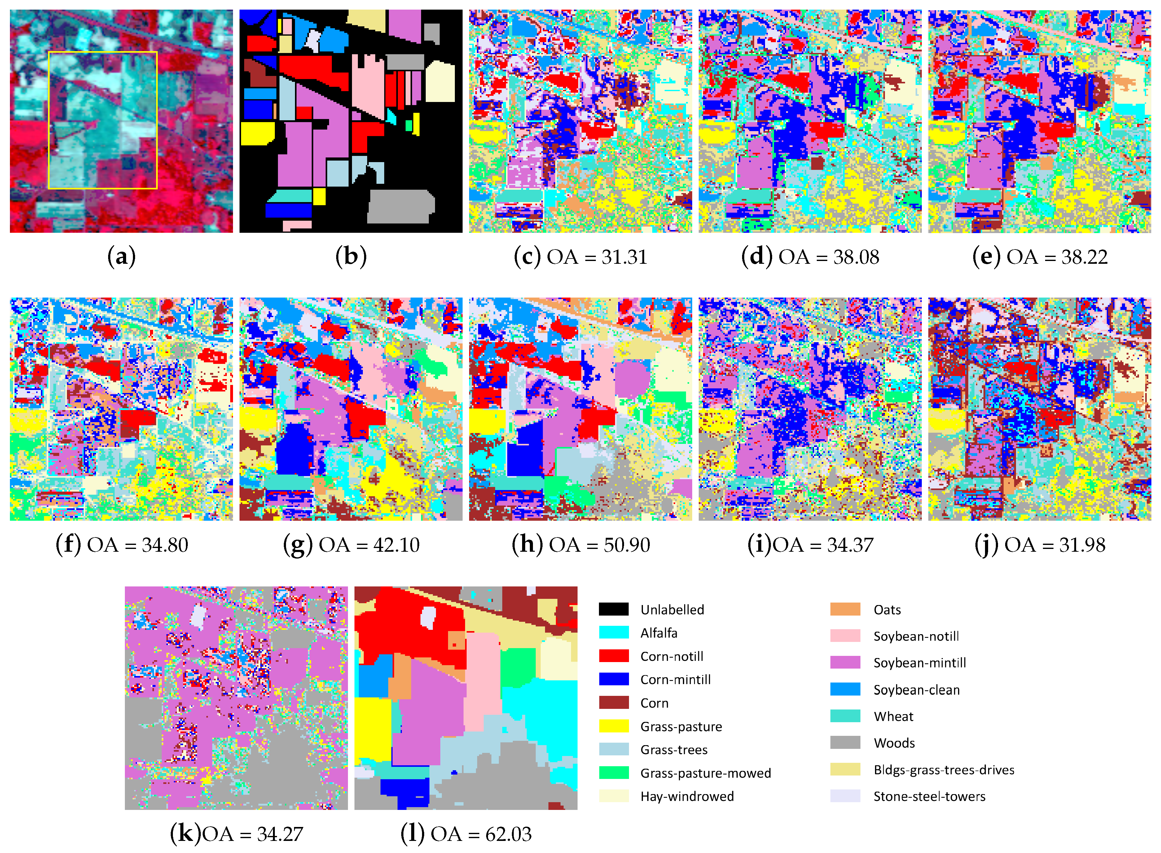
4.2.1. Indian Pines

This image was captured in 1992 by the Airborne/Visible Infrared Imaging Spectrometer (AVIRIS) sensor over the Indian Pines region in North-western Indiana. The image has a spatial resolution of 20 m per pixel, and contains 16 ground-truth classes and 220 spectral reflectance bands in the wavelength range 0.4–2.5 $\mathsf{\mu }$m. The image size is $145\times 145\times 220$. During the test, 20 spectral bands in 104–108, 150–163 and 200 are removed due to water absorption. Figure 3a,b show the false color image and the ground truth of the cropped Indian Pines with the size of $85\times 70$, which includes 4 classes. The complete data set is shown in Figure 5.

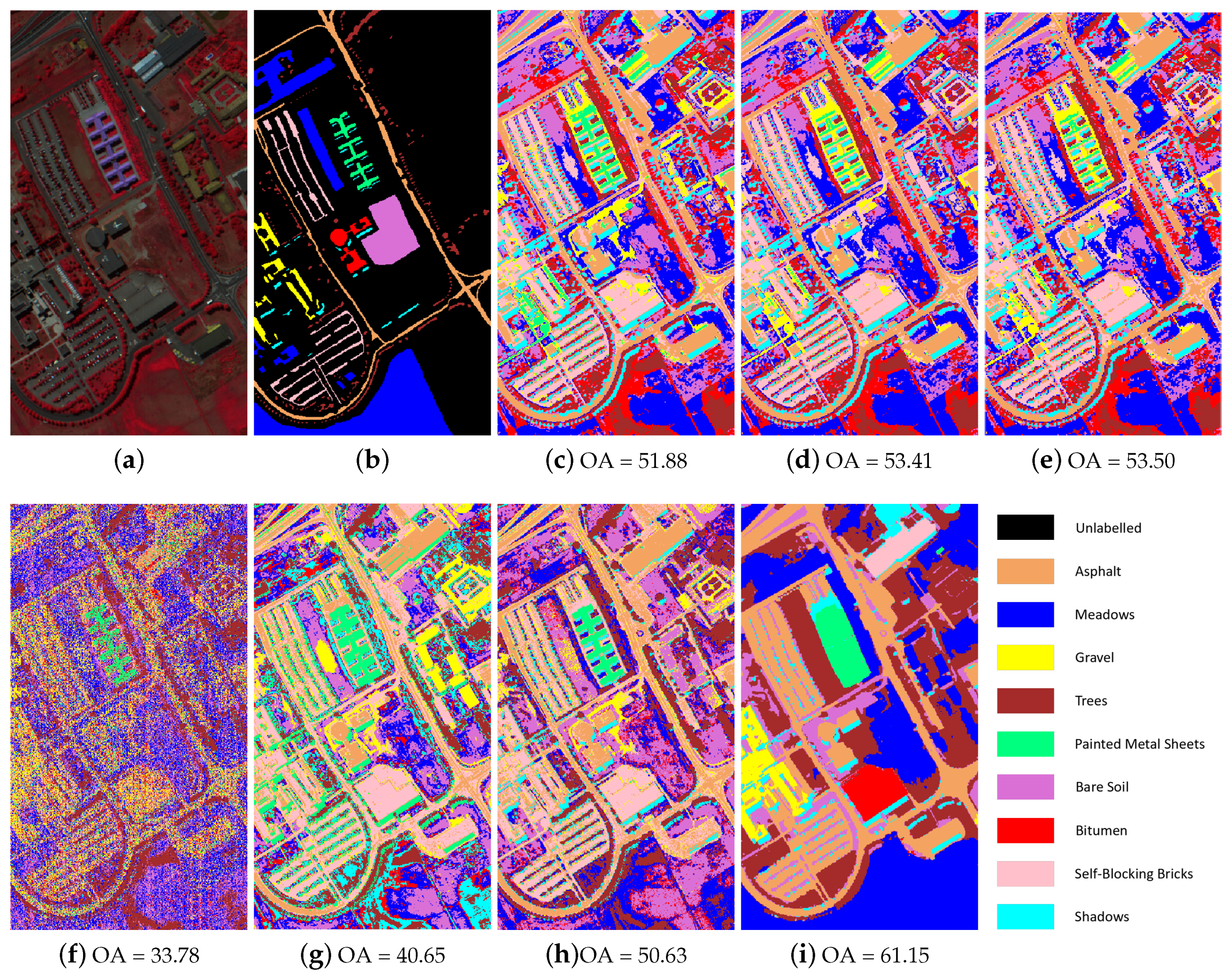
4.2.2. Pavia University

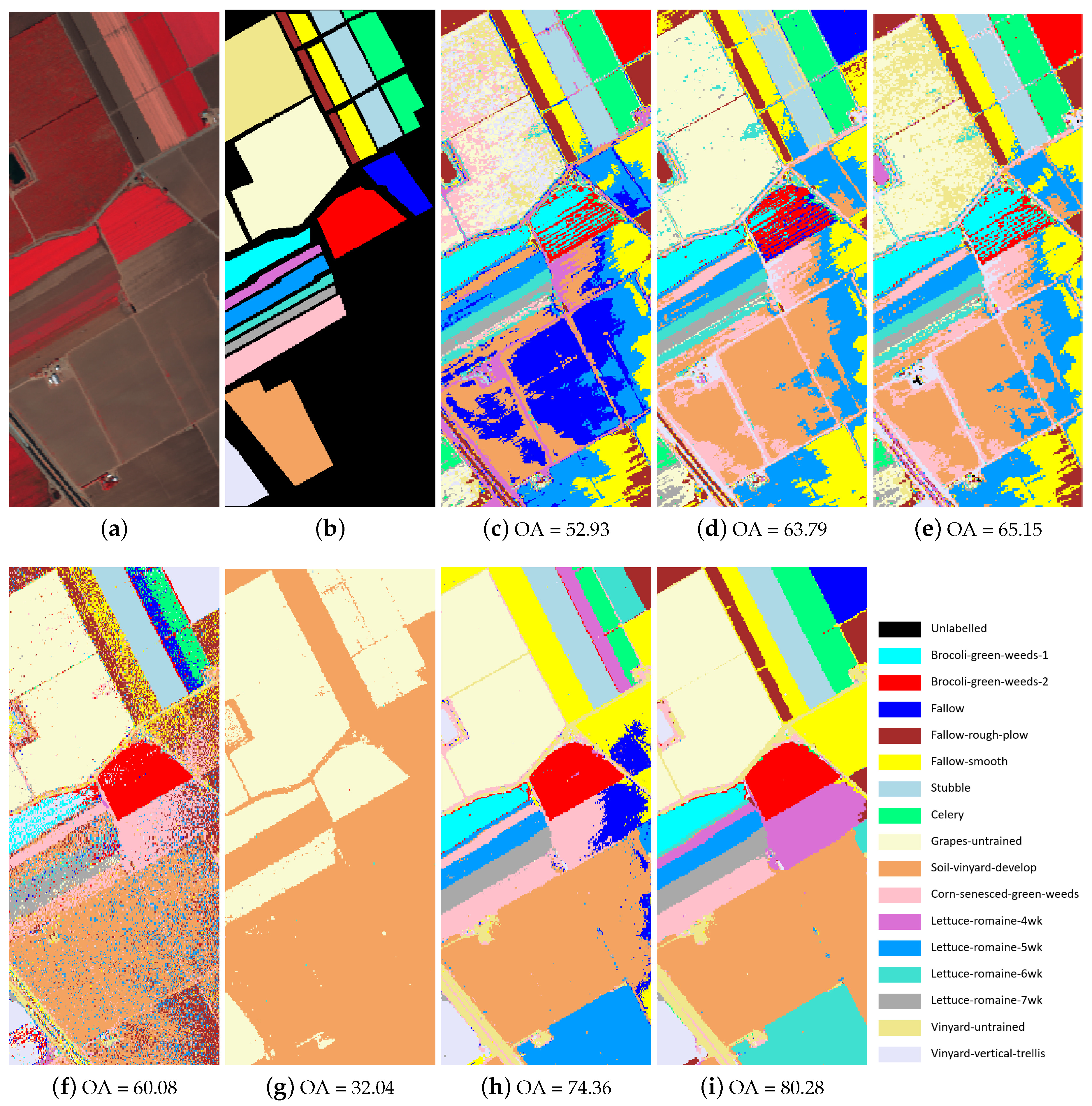
This data was collected by the Reflective Optics System Imaging Spectrometer (ROSIS) sensor during a flight campaign over Pavia, Northern Italy. The typically used image consists of $610\times 340$ pixels, resulting in 207,400 pixels with 103 spectral reflectance bands. The resolution is 1.3 m per pixel and the number of ground-truth classes is 9. The false color image and ground truth are shown in Figure 6a,b.

4.2.3. Salinas

The third image was acquired by the AVIRIS sensor over the Salinas Valley, CA, USA. The geometric resolution is 3.7 m per pixel, and the image size is $512\times 217\times 224$. There are 16 ground-truth classes. Twenty bands in 108–112, 154–167 and 224 are removed due to water absorption. The false color image and ground truth are shown in Figure 7a,b.

4.3. Experiments on the Small HSI

In this part, the experiments are conducted on the data in Figure 3 that is cropped from the original Indian Pines as indicated by the yellow box in Figure 5a. The specific class names and their corresponding clustering results are shown in

Table 1. Clustering results on the parts of Indian Pines.

No.	Class Name	FCM	k-Means	RSC	SSC	L2-SSC	JSSC	SSSC	SSC-OMP	Sketch-SSC	Sketch-SSC-TV
1	Corn-notill	62.39	69.85	69.65	60.00	61.09	74.03	53.31	69.35	62.19	61.41
2	Grass-trees	94.66	53.84	51.10	98.36	99.32	100	89.73	99.86	100	100
3	Soybean-notill	44.13	0	1.23	76.91	79.37	86.20	49.13	44.40	68.80	100
4	Soybean-mintill	63.83	57.59	58.63	50.68	54.89	87.79	63.85	41.68	58.87	93.81
OA(%)		65.34	50.17	50.33	65.11	67.78	86.40	63.28	58.14	68.12	88.46
$\kappa$		0.5118	0.2833	0.2851	0.5296	0.5629	0.8069	0.4772	0.4419	0.5628	0.8342
t (seconds)		5.6	2.5	81	543	624	270	2.2	22	2.8	5.8

, where the best result is marked in bold and the sub-optimal result is underlined.

The results reveal that our proposed Sketch-SSC-TV model achieves the best performance in terms of clustering accuracy and $\kappa$. The optimal parameters of the Sketch-SSC-TV in terms of OA are $\lambda ={10}^{-3},{\lambda }_{tv}={10}^{-2}$. Compared with the classical clustering methods FCM and k-means, the SSC-based methods SSC, L2-SSC, JSSC, Sketch-SSC and Sketch-SSC-TV usually yield higher accuracy, showing the superior capability of SSC model in such clustering task. RSC is a k-means based clustering method, which consists of a sequence of centroid swaps and fine-tuning of the exact centroids with k-means. It shows better performance than k-means in Table 1 in terms of OA and $\kappa$. The number of iterations in RSC is set by default to 5000 in the source code (http://www.uef.fi/web/machine-learning/software), resulting thereby in longer running time than k-means and FCM. The classification accuracy of k-means for the class “Soybean-notill” is zero, which means that all the pixels belonging to class 3 are wrongly assigned to other classes. Compared with the original SSC model, the extensions L2-SSC and JSSC by incorporating different spatial information obtain the improved performance with the higher accuracy, which indicates the importance of spatial information in HSI clustering. It is very interesting and also surprised to find that the proposed Sketch-SSC-TV method yields higher clustering accuracy than the L2-SSC and JSSC methods which not only use the uncompressed self-representation dictionary but also takes the spatial information into account. Compared with the large-scale clustering methods SSSC, SSC-OMP and Sketch-SSC, our method yields significant accuracy improvement of more than 20%. The SSSC model heavily relies on the initially selected samples. So when the data sets are contaminated by noise or much diverse in each class, the performance may be greatly degraded. Compared with the Sketch-SSC model, our method offers significant improvement as well, which demonstrates the effectiveness of our approach.

Figure 4 shows the similarity matrices obtained by different clustering methods. For a better visual comparison, we randomly select 75 samples per class and arrange them in the sequential order by classes. It is known that the ideal similarity matrix should be block-diagonal as only the samples of the same class are connected in the graph [11]. The results in Figure 4 indicate that our method (Figure 4f) preserves such block-diagonal structure best, which is also the main reason why our approach achieves the highest accuracy in the spectral clustering in Table 1. In general, the similarity matrices in Figure 4e,f constructed by KNN are sparser than that by (2) in Figure 4a–c, but surprisingly they achieve comparable or even better spectral clustering performance, demonstrating the efficiency of sparse graph in the spectral clustering. The similarity matrix in Figure 4d is over sparse due to the strict sparsity constraint in the OMP algorithm, leading to the poor clustering performance. It is clearly observed that there are a lot of wrong connections between class 3 and class 4 in Figure 4a–c,e, which consequently results in the low accuracy for class 3 and class 4 as shown in Table 1. While it is less pronounced in Figure 4f, showing much closer block-diagonal structure, which achieves the highest accuracy for class 3 and 4. Such improved graph connectivity mainly benefits from the utilization of TV spatial regularization.

The results in Table 1 show that the SSSC method achieves the shortest computational time. k-means is known to be an efficient clustering algorithm with the complexity of $\mathcal{O}\left(IBcMN\right)$ where I is the number of iterations. The time complexity of SSSC is $\mathcal{O}(I_{1}B{n}^3+I_{2}n{c}^2+MN{n}^2)$, where n is set to 70 in the experiment. k-means took slightly longer running time than SSSC because it needed much more iterations to converge than SSSC on this data set. However, the results on the big data sets such as Pavia University and Salinas shown later indicate that k-means consistently is the fastest algorithm. It is also observed that the computation time t of the SSSC method is increased when the number of initially selected samples becomes larger. Among the clustering methods designed for large-scale data, SSC-OMP takes the longest time. In general, the large-scale clustering methods are much faster than the traditional SSC-based methods, with more than hundred times speed improvement. The reason for the significant speed improvement is that traditional SSC-based methods SSC, L2-SSC and JSSC use the self-representation dictionary $\mathbf{Y}$, which is commonly huge for large-scale data and involves thereby many time-consuming operations of matrix multiplications and inverse calculations on the large dense matrix ${\mathbf{Y}}^T\mathbf{Y}\in {\mathbb{R}}^{MN\times MN}$ in the optimization loop, while scalable clustering methods SSSC, Sketch-SSC and Sketch-SSC-TV employ a compressed dictionary, thus enabling a much lower computational complexity. In our method, the column size of the sketched dictionary $\mathbf{D}$ is 70 so that the cost of matrix multiplications and inverse calculation on the new matrix ${\mathbf{D}}^T\mathbf{D}\in {\mathbb{R}}^{70\times 70}$ in the optimization algorithm is significantly reduced in comparison with that on the huge matrix ${\mathbf{Y}}^T\mathbf{Y}$ in the traditional SSC-based methods. That is why our method only uses 6 seconds to obtain clustering result while the traditional SSC-based methods take around 10 minutes. The computation time of our sketching-based method is comparable to that of FCM and k-means, and hence much smaller than the computation time of the traditional SSC-based methods. Compared with other large-scale clustering methods, the computational cost of the Sketch-SSC-TV is similar.

4.4. Experiments on the Large-Scale HSIs

In this part, we conduct three more experiments on the entire HSIs. Due to the high computational memory requirement of the traditional SSC-based methods on large-scale HSIs, the SSC, L2-SSC and JSSC methods cannot be run on our computer for the Pavia University and Salinas. We estimate the required memory for only saving the large matrix ${\mathbf{Y}}^T\mathbf{Y}$ in the three HSIs by MATLAB as in

Table 2. Required memory for saving ${\mathbf{Y}}^T\mathbf{Y}$ in different HSIs.

	Indian Pines	Pavia University	Salinas
Spatial image size	$145\times 145$	$610\times 340$	$512\times 217$
Matrix size of ${\mathbf{Y}}^T\mathbf{Y}$	21,025 × 21,025	207,400 × 207,400	111,104 × 111,104
Required memory (GB)	3.5	320.5	92

. The required memory for the Pavia University is 320.5 GB without considering the extra memory cost for the operations including matrix multiplications and inverse calculations, which is unaffordable for normal computational devices. We report the experimental results in

Table 3. Clustering accuracy for Indian Pines.

No.	Class Name	FCM	k-Means	RSC	SSC	L2-SSC	JSSC	SSSC	SSC-OMP	Sketch-SSC	Sketch-SSC-TV
1	Alfalfa	23.91	0	17.39	36.96	0	0	14.78	0	7.39	57.83
2	Corn-notill	25.70	28.71	29.06	23.39	43	48.25	25.48	19.33	2.28	33.70
3	Corn-mintill	24.82	44.34	43.49	34.34	20.48	18.19	24.24	35.90	0.53	32.53
4	Corn	6.33	14.35	20.25	9.28	0	0.42	5.91	53.16	2.62	42.53
5	Grass-pasture	43.89	49.69	49.69	65.01	55.49	65.22	46.54	36.02	1.90	65.84
6	Grass-trees	25.75	40.82	44.52	37.95	56.71	75.21	48.49	49.04	12.41	45.18
7	Grass-pasture-mowed	0	71.43	0	0	85.71	75.00	7.14	0	12.86	0
8	Hay-windrowed	89.33	85.15	81.80	55.02	71.13	98.74	56.32	77.41	15.10	100
9	Oats	0	0	30.00	65.00	45	0	6.00	65.00	3.00	20.00
10	Soybean-notill	23.46	18.83	18.42	30.04	58.54	62.04	24.96	27.16	3.48	75.23
11	Soybean-mintill	28.35	38.98	39.55	33.93	37.64	43.34	38.07	23.87	89.42	76.85
12	Soybean-clean	23.61	18.21	17.20	22.26	24.28	44.69	16.42	19.06	3.27	64.99
13	Wheat	99.51	97.07	96.59	96.10	98.54	100	55.71	58.54	5.66	79.61
14	Woods	30.99	41.82	41.50	38.50	38.42	53.12	39.43	41.11	99.81	71.46
15	Bldgs-grass-trees-drives	17.62	18.13	17.36	21.50	16.06	38.08	15.18	11.14	1.40	11.92
16	Stone-steel-towers	59.14	86.02	87.10	19.35	95.70	67.74	25.59	18.28	19.78	79.14
OA		31.31	38.08	38.22	34.80	42.10	50.90	33.24	31.98	36.78	60.48
$\kappa$		0.2556	0.3099	0.3118	0.2864	0.3593	0.4525	0.2563	0.2659	0.2234	0.5575
t (seconds)		74	10	503	16906	20769	18326	9	462	7	26

,

Table 4. Clustering accuracy for Pavia University.

No.	Class Name	FCM	k-Means	RSC	SSC *	L2-SSC *	JSSC *	SSSC	SSC-OMP	Sketch-SSC	Sketch-SSC-TV
1	Asphalt	84.54	90.51	90.63	-	-	-	35.60	59.64	64.88	99.78
2	Meadows	38.61	43.83	44.09	-	-	-	28.47	27.55	42.55	57.25
3	Gravel	7.58	0.10	0.10	-	-	-	11.92	1.05	20.14	19.43
4	Trees	70.33	63.67	64.07	-	-	-	61.29	82.38	91.17	75.05
5	Painted Metal Sheets	74.80	48.25	48.77	-	-	-	62.05	97.10	99.79	100
6	Bare Soil	37.78	32.89	32.49	-	-	-	18.56	31.64	27.94	60.93
7	Bitumen	0	0	0	-	-	-	5.86	0	0.38	0
8	Self-Blocking Bricks	87.48	94.24	93.75	-	-	-	31.48	77.49	65.11	0.15
9	Shadows	99.89	100	100	-	-	-	8.91	0	75.73	73.75
OA		51.88	53.41	53.50	-	-	-	30.13	40.65	49.84	58.71
$\kappa$		0.4238	0.4337	0.4343	-	-	-	0.1794	0.3093	0.3957	0.4858
t (seconds)		209	17	1640	-	-	-	30	72397	838	974

* Note: SSC, L2-SSC and JSSC cannot be implemented on our computer in this data due to the out-of-memory problem.

and

Table 5. Clustering accuracy for Salinas.

No.	Class Name	FCM	k-Means	RSC	SSC *	L2-SSC *	JSSC *	SSSC	SSC-OMP	Sketch-SSC	Sketch-SSC-TV
1	Brocoli-green-weeds-1	99.75	98.36	99.90	-	-	-	66.99	0	99.43	99.94
2	Brocoli-green-weeds-2	39.59	66.56	30.30	-	-	-	88.60	0.05	98.91	99.53
3	Fallow	19.13	0	0.00	-	-	-	28.64	0	11.92	8.21
4	Fallow-rough-plow	99.21	90.32	99.21	-	-	-	50.63	0	19.90	59.83
5	Fallow-smooth	91.67	76.14	92.87	-	-	-	44.20	0	99.45	98.92
6	Stubble	94.44	87.95	94.49	-	-	-	99.50	0.05	99.54	99.55
7	Celery	98.63	97.99	98.21	-	-	-	90.98	0	55.25	82.16
8	Grapes-untrained	34.08	93.60	70.95	-	-	-	58.62	98.82	98.67	98.95
9	Soil-vinyard-develop	57.97	74.13	75.58	-	-	-	77.94	99.92	99.72	99.94
10	Corn-senesced-green-weeds	7.29	30.96	33.10	-	-	-	44.23	0.06	88.04	94.26
11	Lettuce-romaine-4wk	4.12	0	0.00	-	-	-	34.01	0	54.21	56.95
12	Lettuce-romaine-5wk	89.52	91.65	96.11	-	-	-	12.36	0	70.97	90.75
13	Lettuce-romaine-6wk	99.02	98.58	98.80	-	-	-	8.84	0	0	0
14	Lettuce-romaine-7wk	87.38	89.25	88.41	-	-	-	54.04	0	97.78	78.77
15	Vinyard-untrained	30.02	0.01	48.56	-	-	-	28.46	0	0.28	0.30
16	Vinyard-vertical-trellis	12.06	0	0.00	-	-	-	47.58	0	97.61	98.17
OA		52.93	63.79	65.15	-	-	-	57.97	32.04	73.43	77.00
$\kappa$		0.4900	0.5926	0.6116	-	-	-	0.5340	0.1743	0.7007	0.7411
t (seconds)		394	31	1946	-	-	-	37	21831	269	335

* Note: SSC, L2-SSC and JSSC cannot be implemented on our computer in this data due to the out-of-memory problem.

. The clustering maps are shown in Figure 5, Figure 6 and Figure 7. The optimal parameters of the Sketch-SSC-TV model are $\lambda ={10}^{-3},{\lambda }_{tv}={10}^{-1}$ for the Indian Pines, $\lambda =5\times {10}^{-2},{\lambda }_{tv}=5\times {10}^{-1}$ for the Pavia University and $\lambda ={10}^{-3},{\lambda }_{tv}={10}^{-4}$ for the Salinas.

The results in Table 3, Table 4 and Table 5 reveal that our method consistently achieves the highest clustering accuracy in the three HSIs, which confirms its effectiveness. Clustering for the Indian Pines is a very challenging task as some of the spectral signatures from different classes are very close and also parts of the spectrum are highly mixed due to low spatial resolution [20]. As depicted in Table 3 most of the approaches achieve quite low clustering accuracy, while our method yields a much better result with the accuracy of 60.48%.

The FCM, k-means and RSC produce similar accuracy in the Indian Pines and Pavia University, but the k-means is more efficient in terms of computation time than FCM and RSC. The traditional SSC-based methods SSC, L2-SSC and JSSC can be run only on the Indian Pines, however, our method is not only capable of running on all the three large-scale HSIs but also improves clustering performance, which mainly benefits from the exploitation of TV-norm spatial constraint and the sketching technique. Also in Table 3 we can see the computation time of the Sketch-SSC-TV method is significantly reduced by at least 600 times compared to the SSC, L2-SSC and JSSC methods, indicating the efficiency of using a compressed dictionary in our method instead of using the large self-representation dictionary. For the clustering methods designed for large-scale data, SSC-OMP uses much longer time than SSSC, Sketch-SSC and our method. The reason is that the sparse coding for each sample is performed in series. The computational time can be reduced by running simulation in parallel. Compared with the SSC clustering map in Figure 5f, the L2-SSC, JSSC and Sketch-SSC-TV methods have less impulse noise in the clustering maps, which is due to the use of spatial information to promote the connectivity between neighbouring pixels, leading to a more robust similarity matrix. The clustering results in Table 4 show that the accuracy of our method on “Self-Blocking-Bricks” is much lower than that of the reference methods. This can mainly be attributed to the over-smoothed clustering results as shown in Figure 6i, where the “Painted Metal Sheets” and the neighbouring “Self-Blocking-Bricks” are merged. However, this can be alleviated by relaxing the spatial constraint with a smaller ${\lambda }_{tv}$. A possible risk is the reduced overall accuracy.

The large-scale clustering methods SSSC and SSC-OMP typically yield worse performance in terms of accuracy than the k-means and RSC method in the three large-scale HSIs, which indicates the limitation of their performance in HSI clustering. In Figure 5i, Figure 6f and Figure 7f the SSSC clustering maps are seriously deteriorated by the impulse noise, which is caused by the limited discriminative information in the spectral domain. The SSC-OMP method also suffers from the same problem for the Indian Pines and Pavia University as shown in Figure 5j and Figure 6g. Compared with the Sketch-SSC method, our method achieves significant improvement in terms of accuracy in the three large-scale HSIs, especially in the Indian Pines with the accuracy enhancement of 23.7%. The cost is a slight increase of computational time that comes from the TV-norm regularization. The Sketch-SSC model also suffers from the same impulse noise problem to the SSSC and SSC-OMP approaches in the clustering maps as shown in Figure 5k, Figure 6h and Figure 7h, while in our method such a problem is greatly alleviated as connections between neighbouring pixels are strengthened by the TV-norm constraint.

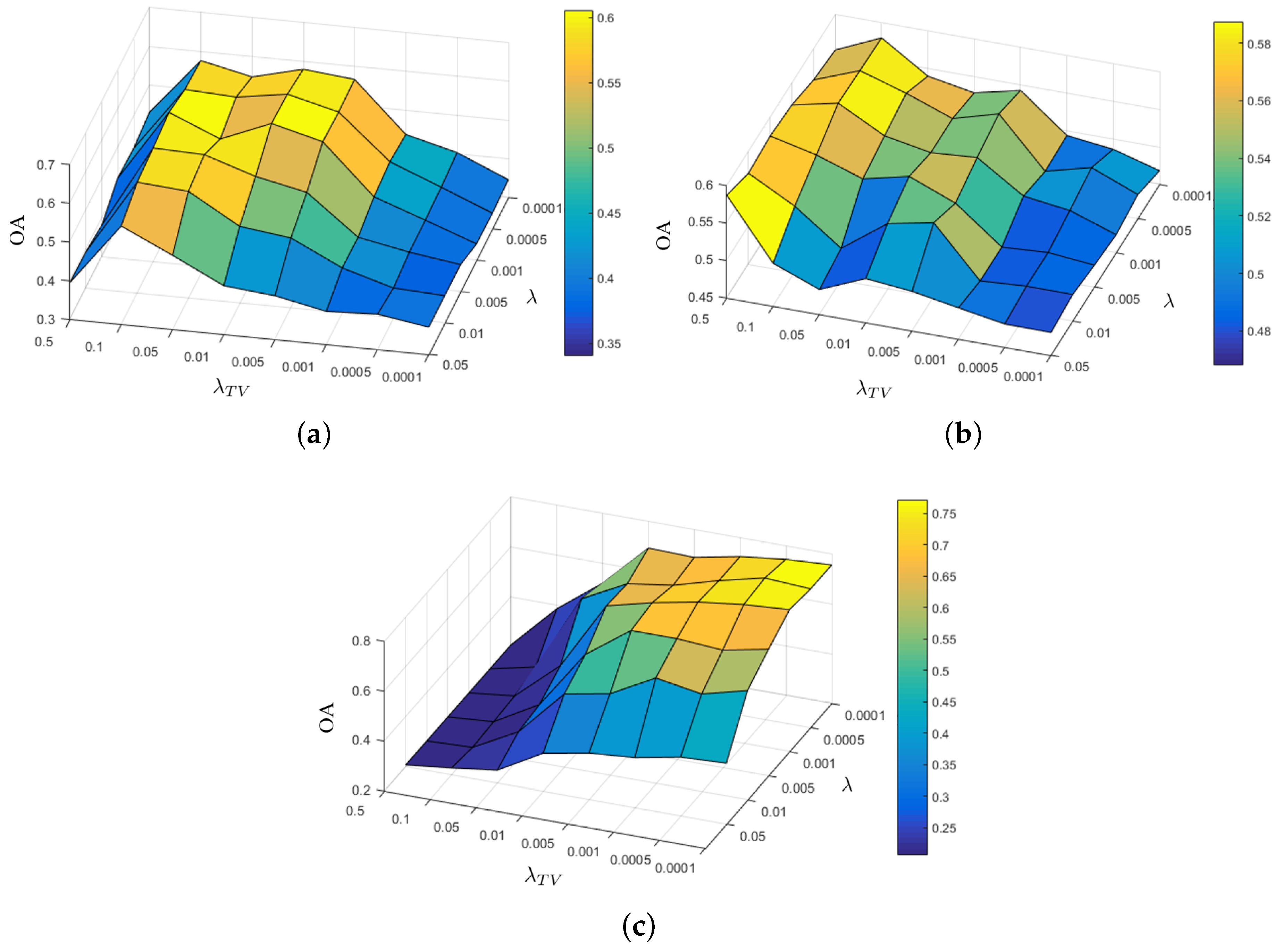
4.5. Analysis of Parameters

In this part, we analyse the effect of the parameters $\lambda ,{\lambda }_{tv},n$ and k on the clustering performance of the Sketch-SSC-TV method in the large-scale HSIs.

4.5.1. Effect of $\lambda$ and ${\lambda }_{tv}$

$\lambda$ and ${\lambda }_{tv}$ in (8) controls the sparsity level and spatial constraint of the sparse matrix, respectively, which are two important parameters in the model. Let $\lambda$ be varied in the range of $\{1\times {10}^{-4},5\times {10}^{-4},1\times {10}^{-3},5\times {10}^{-3},1\times {10}^{-2},5\times {10}^{-2}\}$ and ${\lambda }_{tv}$ in the range of $\{1\times {10}^{-4},5\times {10}^{-4},1\times {10}^{-3},5\times {10}^{-3},1\times {10}^{-2},5\times {10}^{-2},1\times {10}^{-1},5\times {10}^{-1}\}$. The clustering results with respect to $\lambda$ and ${\lambda }_{tv}$ are shown in Figure 8 for the three large-scale HSIs. The results indicate that the clustering performance is more stable with respect to $\lambda$ than ${\lambda }_{tv}$. According to the experimental results, we recommend to set $\lambda ={10}^{-3}$ for all the data. For the parameter ${\lambda }_{tv}$, the value may be different for different data sets, but the clustering accuracy is stable and superior over other methods in a wide range, that is, when ${\lambda }_{tv}\in [5\times {10}^{-3},{10}^{-1}]$ for the Indian Pines, ${\lambda }_{tv}\in [5\times {10}^{-3},5\times {10}^{-1}]$ for the Pavia University and ${\lambda }_{tv}\in [{10}^{-4},5\times {10}^{-3}]$ for the Salinas. The results of Salinas in Figure 8c are quite different with those of the Indian Pines and Pavia University. For the Salinas when the values of ${\lambda }_{tv}$ and $\lambda$ are similar, the results typically show better performance, which means the sparsity constraint and spatial constraint are equally important. In contrast, for the Indian Pines and Pavia University our method achieves better performance when ${\lambda }_{tv}$ is larger than $\lambda$, indicating the spatial constraint is more important than the sparsity. The reason may lie in different types of HSIs and different levels of data quality. As each crop in the Salinas is planted regularly in block, there are more homogeneous regions and less edge than the Indian Pines and Pavia University, resulting in much smaller value of the TV-norm in Salinas. In addition, due to high data quality of the Salinas spatial information may be less important than that in the other two HSIs. Thus a lager value of ${\lambda }_{tv}$ can make the clustering result over smoothing, leading to a lower accuracy. Among the three constraints of Sketch-SSC-TV model, the data fidelity term is most important for the Salinas. Overall, based on the results in Figure 8 our method is robust and stable with respect to $\lambda$ and ${\lambda }_{tv}$.

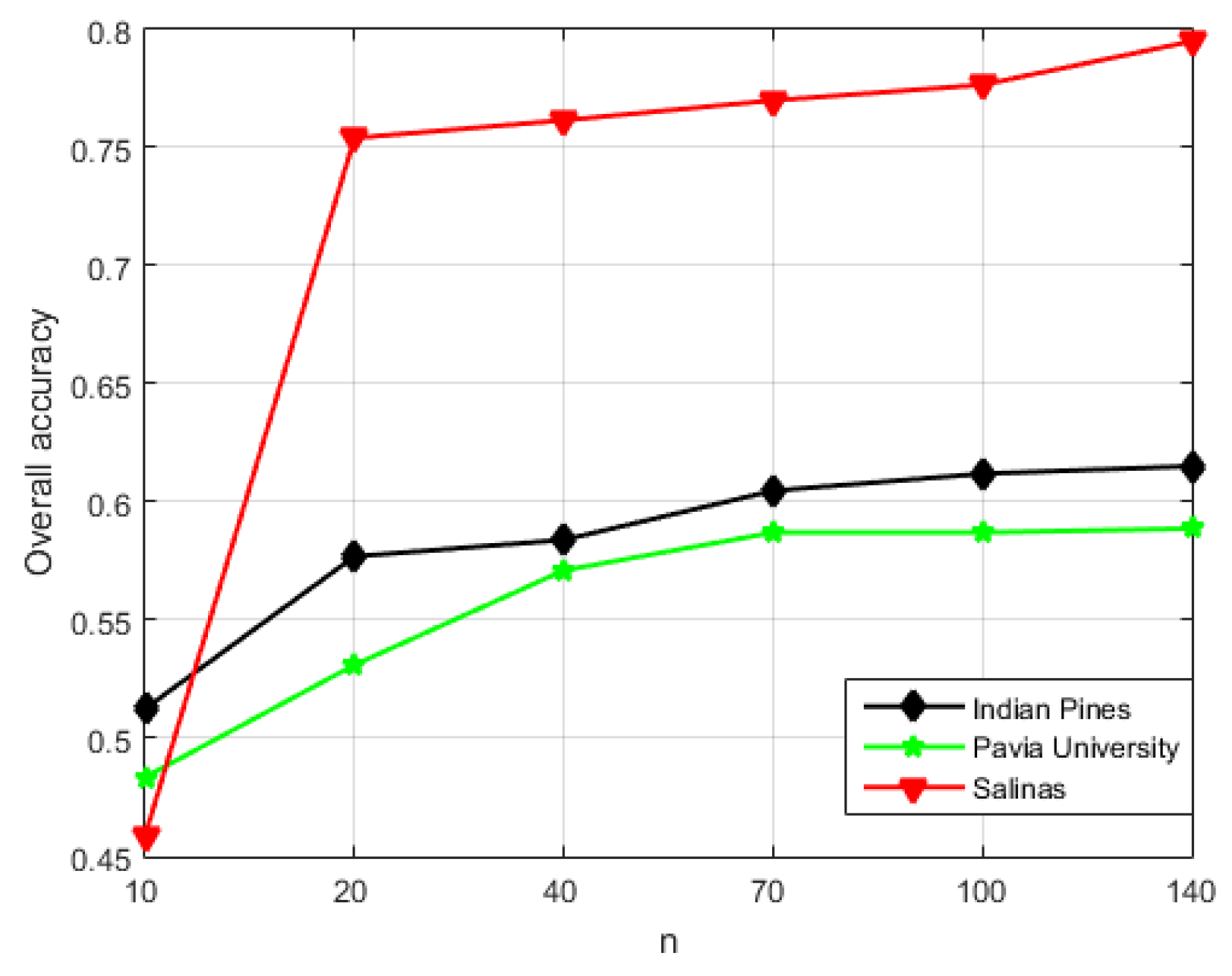
4.5.2. Effect of the Parameter n

n is the number of columns of the sketching matrix $\mathbf{R}$, which decides the sketched dictionary size and also the computation efficiency of the proposed method. We vary n in the range of $\{10,20,40,70,100,140\}$ for the three large-scale HSIs. The results are reported in Figure 9, which shows that a larger n typically can result in a better clustering result. The reason is that a larger sketched dictionary can better preserve the original column space of the input data. For the Indian Pines and Salinas, the number of classes is 16. When $n=10$, the sketched dictionary cannot well represent the input data space, which results in the drop of accuracy compared to that when $n=20$. It is also revealed in Figure 9 that a small value of n (20 for example) is able to obtain satisfying clustering performance in the three HSIs, which coincides with the fact that the data of HSIs actually lies in a low dimensional subspace.

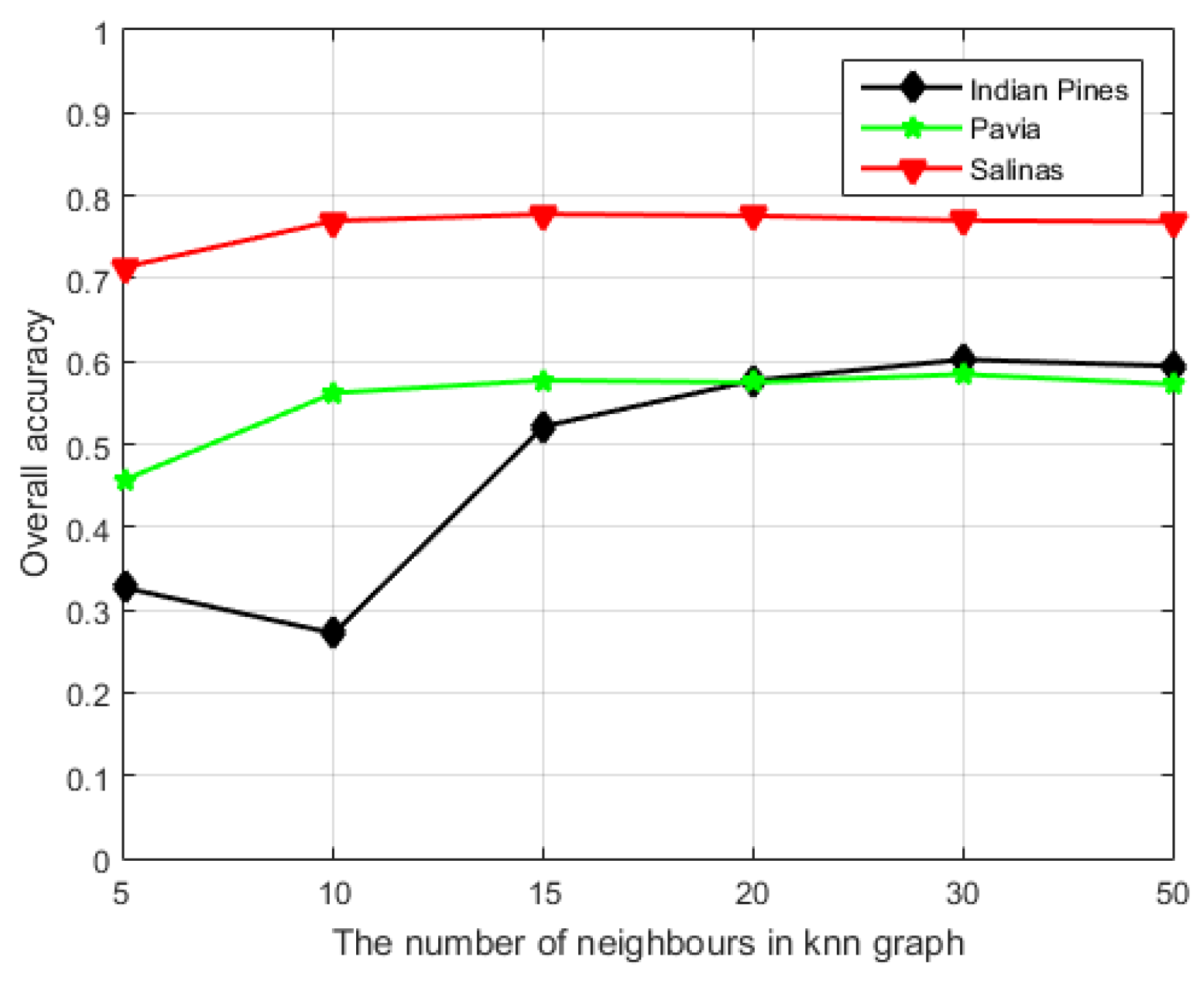
4.5.3. Effect of the Parameter k

We investigate the effect of the number of neighbours k on the clustering performance of our method by varying k in the range of $\{5,10,15,20,30,50\}$ for the three large-scale HSIs. The results shown in Figure 10 reveal that a larger k yields a higher clustering accuracy in general. The accuracy curves with $k<20$ rise more significantly than those with $k\ge 20$ in the three HSIs. When $k\ge 20$, the accuracy becomes much more stable. Based on the results, we set the value of k to 30 in this paper.

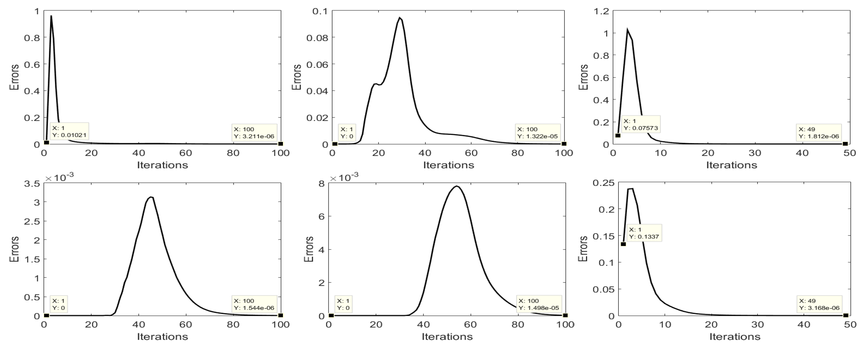
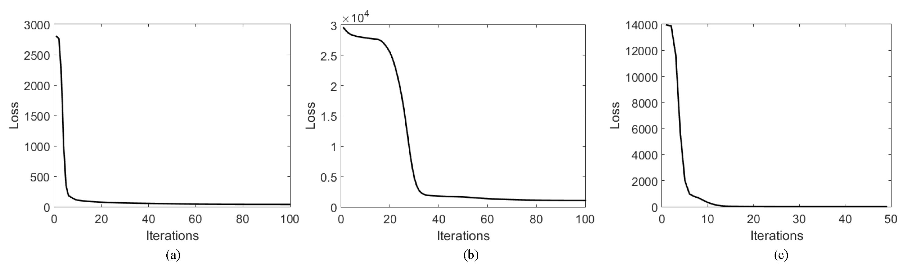
4.6. Experimental Convergence Analysis

Figure 11 shows the squared Frobenius norm of the differences in $\mathbf{Z}$ and $\mathbf{U}$ values in each two subsequent iterations: $\parallel {\mathbf{Z}}^{r+1}-{\mathbf{Z}}^r{\parallel }_F^2$ and $\parallel {\mathbf{U}}^{r+1}-{\mathbf{U}}^r{\parallel }_F^2$. We refer to these distances between the values of $\mathbf{Z}$ and $\mathbf{U}$ in two successive iterations as updating errors. The results show that the updating errors after a sufficient number of iterations tend to a very small value, meaning that the solutions of $\mathbf{Z}$ and $\mathbf{U}$ become stable eventually. Moreover, on all three datasets, the updating errors decline monotonically after certain iterations. Thus, we have ${lim}_{r\to \infty }\mu ({\mathbf{Z}}^{r+1}-{\mathbf{Z}}^r)=\mathbf{0}$ and ${lim}_{r\to \infty }\mu ({\mathbf{U}}^{r+1}-{\mathbf{U}}^r)=\mathbf{0}$, where $\mu$ is a constant. This empirically demonstrates that the conditions in Theorem 1 are satisfied for all three analysed datasets, and it is thus reasonably to assume that they will be satisfied in a similar manner for most other HSIs in practice. It can be observed that the updating errors of $\mathbf{Z}$ and $\mathbf{U}$ in some datasets are zero at the beginning, which is mainly caused by the small values of ${\mathbf{A}}^{r+1}+{\mathbf{Y}}_2^r/\mu$ in (18) and ${\mathbf{HA}}^{{(r+1)}^T}+{\mathbf{Y}}_3^r/\mu$ in (22) at the first several iterations, leading to the output of zero matrices in the thresholding operator ${\mathcal{R}}_{△}(·)$. After certain number of iterations, their values increase and the output of thresholding operator is no longer zero, resulting in a temporary increase of updating errors, as shown in Figure 11. But finally they tend to a value that is close to zero.

The diagrams in Figure 12 show the evolution of the objective function values with respect to the number of iterations. The results reveal that the objective function is monotonically decreasing to a stable level in the three data sets, demonstrating the practical convergence of our optimization algorithm. Especially, the curves in Figure 12a,c drop sharply in the first few iterations and then become saturated. The results coincide with the aforementioned theoretical convergence analysis.

5. Conclusions

In this paper, the problem of large-scale HSIs clustering based on the SSC model is addressed for the first time, and a novel clustering method, namely Sketch-SSC-TV, is proposed to incorporates a random projection based sketching technique to significantly reduce the number of optimization variables. In addition, a TV-norm constraint on the sparse coefficient matrix promotes the dependencies between neighbouring pixels, which enhances the block-diagonal structure of the similarity matrix, improving thereby the performance of spectral clustering. We derived an efficient solver based on the ADMM algorithm for the resulting model and also we proved its convergence property theoretically. Unlike the traditional SSC-based methods which cannot be applied on large-scale HSIs due to extremely high computational burden, the proposed method is not only applicable on big data sets but also able to achieve a high level of clustering accuracy. The extensive experimental results clearly demonstrate that our method outperforms the state-of-the-art clustering methods.

References

1. Zhang, Y.; Du, B.; Zhang, Y.; Zhang, L. Spatially Adaptive Sparse Representation for Target Detection in Hyperspectral Images. IEEE Geosci. Remote Sens. Lett. 2017, 14, 1923–1927. [Google Scholar] [CrossRef]
2. Wu, K.; Xu, G.; Zhang, Y.; Du, B. Hyperspectral image target detection via integrated background suppression with adaptive weight selection. Neurocomputing 2018, 315, 59–67. [Google Scholar] [CrossRef]
3. Camps-Valls, G.; Tuia, D.; Bruzzone, L.; Benediktsson, J.A. Advances in hyperspectral image classification: Earth monitoring with statistical learning methods. IEEE Signal Process. Mag. 2014, 31, 45–54. [Google Scholar] [CrossRef] [Green Version]
4. Eismann, M.T.; Stocker, A.D.; Nasrabadi, N.M. Automated hyperspectral cueing for civilian search and rescue. Proc. IEEE 2009, 97, 1031–1055. [Google Scholar] [CrossRef]
5. Bezdek, J.C. Pattern Recognition with Fuzzy Objective Function Algorithms; Springer: Berlin, Germany, 2013. [Google Scholar]
6. Lloyd, S. Least squares quantization in PCM. IEEE Trans. Inf. Theory 1982, 28, 129–137. [Google Scholar] [CrossRef]
7. Arthur, D.; Vassilvitskii, S. k-means++: The advantages of careful seeding. In Proceedings of the Eighteenth Annual ACM-SIAM Symposium on Discrete Algorithms (SODA), New Orleans, LA, USA, 7–9 January 2007; pp. 1027–1035. [Google Scholar]
8. Chen, G.; Lerman, G. Spectral curvature clustering (SCC). Int. J. Comput. Vis. 2009, 81, 317–330. [Google Scholar] [CrossRef] [Green Version]
9. Dyer, E.L.; Sankaranarayanan, A.C.; Baraniuk, R.G. Greedy feature selection for subspace clustering. J. Mach. Learn Res. (JMLR) 2013, 14, 2487–2517. [Google Scholar]
10. Elhamifar, E.; Vidal, R. Sparse subspace clustering. In Proceedings of the 2009 IEEE Conference on Computer Vision and Pattern Recognition, Miami, FL, USA, 20–25 June 2009; pp. 2790–2797. [Google Scholar]
11. Elhamifar, E.; Vidal, R. Sparse subspace clustering: Algorithm, theory, and applications. IEEE Trans. Pattern Anal. Mach. Intell. 2013, 35, 2765–2781. [Google Scholar] [CrossRef] [Green Version]
12. Liu, G.; Lin, Z.; Yan, S.; Sun, J.; Yu, Y.; Ma, Y. Robust recovery of subspace structures by low-rank representation. IEEE Trans. Pattern Anal. Mach. Intell. 2013, 35, 171–184. [Google Scholar] [CrossRef] [Green Version]
13. Park, D.; Caramanis, C.; Sanghavi, S. Greedy subspace clustering. In Advances in Neural Information Processing Systems; MIT Press: Cambridge, MA, USA, 2014; pp. 2753–2761. [Google Scholar]
14. Vidal, R. Subspace clustering. IEEE Signal Process. Mag. 2011, 28, 52–68. [Google Scholar] [CrossRef]
15. Deerwester, S.; Dumais, S.T.; Furnas, G.W.; Landauer, T.K.; Harshman, R. Indexing by latent semantic analysis. J. Am. Soc. Inform. Sci. 1990, 41, 391–407. [Google Scholar] [CrossRef]
16. Zhang, T.; Szlam, A.; Wang, Y.; Lerman, G. Hybrid linear modeling via local best-fit flats. Int. J. Comput. Vis. 2012, 100, 217–240. [Google Scholar] [CrossRef] [Green Version]
17. Goh, A.; Vidal, R. Segmenting motions of different types by unsupervised manifold clustering. In Proceedings of the 2007 IEEE Conference on Computer Vision and Pattern Recognition, Minneapolis, MN, USA, 17–22 June 2007; pp. 1–6. [Google Scholar]
18. Guo, Y.; Gao, J.; Li, F. Spatial subspace clustering for drill hole spectral data. J. Appl. Remote Sens. 2014, 8, 083644. [Google Scholar] [CrossRef]
19. Guo, Y.; Gao, J.; Li, F. Random spatial subspace clustering. Knowl.-Based Syst. 2015, 74, 106–118. [Google Scholar] [CrossRef]
20. Zhang, H.; Zhai, H.; Zhang, L.; Li, P. Spectral–spatial sparse subspace clustering for hyperspectral remote sensing images. IEEE Trans. Geosci. Remote Sens. 2016, 54, 3672–3684. [Google Scholar] [CrossRef]
21. Zhai, H.; Zhang, H.; Xu, X.; Zhang, L.; Li, P. Kernel Sparse Subspace Clustering with a Spatial Max Pooling Operation for Hyperspectral Remote Sensing Data Interpretation. Remote Sens. 2017, 9, 335. [Google Scholar] [CrossRef] [Green Version]
22. Zhai, H.; Zhang, H.; Zhang, L.; Li, P.; Plaza, A. A new sparse subspace clustering algorithm for hyperspectral remote sensing imagery. IEEE Geosci. Remote Sens. Lett. 2017, 14, 43–47. [Google Scholar] [CrossRef]
23. Huang, S.; Zhang, H.; Pižurica, A. Joint Sparsity Based Sparse Subspace Clustering for Hyperspectral Images. In Proceedings of the 2018 25th IEEE International Conference on Image Processing (ICIP), Athens, Greece, 7–10 October 2018; pp. 3878–3882. [Google Scholar]
24. Zhai, H.; Zhang, H.; Zhang, L.; Li, P. Total Variation Regularized Collaborative Representation Clustering with a Locally Adaptive Dictionary for Hyperspectral Imagery. IEEE Trans. Geosci. Remote Sens. 2018, 57, 166–180. [Google Scholar] [CrossRef]
25. Huang, S.; Zhang, H.; Pižurica, A. Semisupervised Sparse Subspace Clustering Method with a Joint Sparsity Constraint for Hyperspectral Remote Sensing Images. IEEE J. Sel. Top. Appl. Earth Observ. Remote Sens. 2019, 12, 989–999. [Google Scholar] [CrossRef]
26. Wang, R.; Nie, F.; Wang, Z.; He, F.; Li, X. Scalable Graph-Based Clustering with Nonnegative Relaxation for Large Hyperspectral Image. IEEE Trans. Geosci. Remote Sens. 2019, 57, 7352–7364. [Google Scholar] [CrossRef]
27. Huang, S.; Zhang, H.; Pižurica, A. Landmark-Based Large-Scale Sparse Subspace Clustering Method for Hyperspectral Images. In Proceedings of the IGARSS 2019 IEEE International Geoscience and Remote Sensing Symposium, Yokohama, Japan, 28 July–2 August 2019; pp. 799–802. [Google Scholar]
28. Peng, X.; Zhang, L.; Yi, Z. Scalable sparse subspace clustering. In Proceedings of the IEEE Conference on Computer Vision and Pattern Recognition, Portland, United States, 25–27 June 2013; pp. 430–437. [Google Scholar]
29. You, C.; Robinson, D.; Vidal, R. Scalable sparse subspace clustering by orthogonal matching pursuit. In Proceedings of the IEEE Conference on Computer Vision and Pattern Recognition, Las Vegas, United States, 26 June–1 July 2016; pp. 3918–3927. [Google Scholar]
30. Traganitis, P.A.; Giannakis, G.B. Sketched subspace clustering. IEEE Trans. Signal Process. 2018, 66, 1663–1675. [Google Scholar] [CrossRef]
31. Boyd, S.; Parikh, N.; Chu, E.; Peleato, B.; Eckstein, J. Distributed optimization and statistical learning via the alternating direction method of multipliers. Found. Trends Mach. Learn. 2011, 3, 1–122. [Google Scholar] [CrossRef]
32. Von Luxburg, U. A tutorial on spectral clustering. Stat. Comput. 2007, 17, 395–416. [Google Scholar] [CrossRef]
33. Ng, A.Y.; Jordan, M.I.; Weiss, Y. On spectral clustering: Analysis and an algorithm. In Proc of the 14th International Conference on Neural Information Processing Systems: Natural and Synthetic; MIT Press: Cambridge, MA, USA, 2001; pp. 849–856. [Google Scholar]
34. Zhang, H.; Li, J.; Huang, Y.; Zhang, L. A nonlocal weighted joint sparse representation classification method for hyperspectral imagery. IEEE J. Sel. Top. Appl. Earth Observ. Remote Sens. 2014, 7, 2056–2065. [Google Scholar] [CrossRef]
35. Li, W.; Du, Q. Joint within-class collaborative representation for hyperspectral image classification. IEEE J. Sel. Top. Appl. Earth Observ. Remote Sens. 2014, 7, 2200–2208. [Google Scholar] [CrossRef]
36. Xue, J.; Zhao, Y.; Liao, W.; Chan, J.C. Nonlocal Low-Rank Regularized Tensor Decomposition for Hyperspectral Image Denoising. IEEE Trans. Geosci. Remote Sens. 2019, 57, 5174–5189. [Google Scholar] [CrossRef]
37. Luo, F.; Du, B.; Zhang, L.; Zhang, L.; Tao, D. Feature learning using spatial-spectral hypergraph discriminant analysis for hyperspectral image. IEEE Trans. Cybern. 2018, 49, 2406–2419. [Google Scholar] [CrossRef]
38. Xu, J.; Huang, N.; Xiao, L. Spectral-spatial subspace clustering for hyperspectral images via modulated low-rank representation. In Proceedings of the 2017 IEEE International Geoscience and Remote Sensing Symposium (IGARSS), Fort Worth, TX, USA, 23–28 July 2017; pp. 3202–3205. [Google Scholar]
39. Huang, S.; Zhang, H.; Pižurica, A. A Robust Sparse Representation Model for Hyperspectral Image Classification. Sensors 2017, 17, 2087. [Google Scholar] [CrossRef] [Green Version]
40. Mei, S.; Hou, J.; Chen, J.; Chau, L.P.; Du, Q. Simultaneous Spatial and Spectral Low-Rank Representation of Hyperspectral Images for Classification. IEEE Trans. Geosci. Remote Sens. 2018, 56, 2872–2886. [Google Scholar] [CrossRef]
41. Zhai, H.; Zhang, H.; Zhang, L.; Li, P. Reweighted mass center based object-oriented sparse subspace clustering for hyperspectral images. J. Appl. Remote Sens. 2016, 10, 046014. [Google Scholar] [CrossRef]
42. Yan, Q.; Ding, Y.; Xia, Y.; Chong, Y.; Zheng, C. Class-Probability Propagation of Supervised Information Based on Sparse Subspace Clustering for Hyperspectral Images. Remote Sens. 2017, 9, 1017. [Google Scholar] [CrossRef] [Green Version]
43. Iordache, M.D.; Bioucas-Dias, J.M.; Plaza, A. Total variation spatial regularization for sparse hyperspectral unmixing. IEEE Trans. Geosci. Remote Sens. 2012, 50, 4484–4502. [Google Scholar] [CrossRef] [Green Version]
44. Chen, J.; Richard, C.; Honeine, P. Nonlinear Estimation of Material Abundances in Hyperspectral Images with 1-Norm Spatial Regularization. IEEE Trans. Geosci. Remote Sens. 2014, 52, 2654–2665. [Google Scholar] [CrossRef]
45. Simões, M.; Bioucas-Dias, J.; Almeida, L.B.; Chanussot, J. A convex formulation for hyperspectral image superresolution via subspace-based regularization. IEEE Trans. Geosci. Remote Sens. 2015, 53, 3373–3388. [Google Scholar] [CrossRef] [Green Version]
46. He, W.; Zhang, H.; Zhang, L.; Shen, H. Total-variation-regularized low-rank matrix factorization for hyperspectral image restoration. IEEE Trans. Geosci. Remote Sens. 2016, 54, 178–188. [Google Scholar] [CrossRef]
47. He, W.; Zhang, H.; Shen, H.; Zhang, L. Hyperspectral Image Denoising Using Local Low-Rank Matrix Recovery and Global Spatial–Spectral Total Variation. IEEE J. Sel. Topics Appl. Earth Observ. Remote Sens. 2018, 11, 713–729. [Google Scholar] [CrossRef]
48. Liu, H.; Sun, P.; Du, Q.; Wu, Z.; Wei, Z. Hyperspectral Image Restoration Based on Low-Rank Recovery with a Local Neighborhood Weighted Spectral-Spatial Total Variation Model. IEEE Trans. Geosci. Remote Sens. 2018, 57, 1409–1422. [Google Scholar] [CrossRef]
49. Boutsidis, C.; Zouzias, A.; Mahoney, M.W.; Drineas, P. Randomized dimensionality reduction for k-means clustering. IEEE Trans. Inf. Theory 2015, 61, 1045–1062. [Google Scholar] [CrossRef] [Green Version]
50. Indyk, P.; Motwani, R. Approximate nearest neighbors: Towards removing the curse of dimensionality. In Proceedings of the Thirtieth Annual ACM Symposium on Theory of Computing, Dallas, TX, USA, 23–26 May 1998; pp. 604–613. [Google Scholar]
51. Gong, Y.; Lazebnik, S.; Gordo, A.; Perronnin, F. Iterative quantization: A procrustean approach to learning binary codes for large-scale image retrieval. IEEE Trans. Pattern Anal. Mach. Intell. 2013, 35, 2916–2929. [Google Scholar] [CrossRef] [Green Version]
52. Park, Y.; Park, S.; Lee, S.g.; Jung, W. Greedy filtering: A scalable algorithm for k-nearest neighbor graph construction. In International Conference on Database Systems for Advanced Applications; Springer: Cham, Switzerland, 2014; pp. 327–341. [Google Scholar]
53. Glowinski, R.; Le Tallec, P. Augmented Lagrangian and Operator-splitting Methods in Nonlinear Mechanics; SIAM: Philadelphia, PA, USA, 1989; Volume 9. [Google Scholar]
54. Esser, E. Applications of Lagrangian-based alternating direction methods and connections to split Bregman. CAM Rep. 2009, 9, 31. [Google Scholar]
55. Chen, C.; He, B.; Ye, Y.; Yuan, X. The direct extension of ADMM for multi-block convex minimization problems is not necessarily convergent. Math. Program. 2016, 155, 57–79. [Google Scholar] [CrossRef]
56. Lin, Z.; Chen, M.; Ma, Y. The augmented lagrange multiplier method for exact recovery of corrupted low-rank matrices. arXiv 2010, arXiv:1009.5055. [Google Scholar]
57. Bartle, R.G.; Sherbert, D.R. Introduction to Real Analysis; Wiley: New York, NY, USA, 2000; Volume 2. [Google Scholar]
58. Bertsekas, D.P. Nonlinear programming. J. Oper. Res. Soc. 1997, 48, 334. [Google Scholar] [CrossRef]
59. Fang, X.; Teng, S.; Lai, Z.; He, Z.; Xie, S.; Wong, W.K. Robust latent subspace learning for image classification. IEEE Trans. Neural Netw. Learn. Syst. 2017, 29, 2502–2515. [Google Scholar] [CrossRef] [PubMed]
60. Xue, J.; Zhao, Y.; Liao, W.; Chan, J.C.; Kong, S.G. Enhanced Sparsity Prior Model for Low-Rank Tensor Completion. IEEE Trans. Neural Netw. Learn. Syst. 2019. [Google Scholar] [CrossRef] [PubMed]
61. Shen, Y.; Wen, Z.; Zhang, Y. Augmented Lagrangian alternating direction method for matrix separation based on low-rank factorization. Optim. Methods Softw. 2014, 29, 239–263. [Google Scholar] [CrossRef] [Green Version]
62. Fränti, P. Efficiency of random swap clustering. J. Big Data 2018, 5, 13. [Google Scholar] [CrossRef]
63. Lovász, L.; Plummer, M.D. Matching Theory; American Mathematical Soc.: Amsterdam, The Netherlands, 1986. [Google Scholar]
64. Rezaei, M.; Fränti, P. Set matching measures for external cluster validity. IEEE Trans. Knowl. Data Eng. 2016, 28, 2173–2186. [Google Scholar] [CrossRef]
65. Powers, D.M. Evaluation: From precision, recall and F-measure to ROC, informedness, markedness and correlation. J. Mach. Learn. Tech. 2011. [Google Scholar]
Figure 1. A motivation for applying the TV norm in the sparse subspace clustering (SSC) model. In the ideal case, coefficient matrices of pixels in hyperspectral images (HSIs) should be piece-wise smooth in local region and have similar edges to the original HSI, which becomes apparent after reshaping them to a 3-D cube. Observe that each M × N slice in this cube corresponds to one row in the 2-D matrix C and resembles the spatial structures in the original HSI. In order to preserve such smoothness in local regions and edge structure of the coefficient matrix, the TV spatial constraint is employed.
Remotesensing 12 00775 g001
Figure 2. Illustration of the traditional SSC-based models (top) and the sketched SSC model (bottom) where C and A are two sparse coefficient matrices to be computed and R is a random matrix for sketching.
Remotesensing 12 00775 g002
Figure 3. The false color image (a) and the corresponding ground truth (b) of the tested Indian Pines.
Remotesensing 12 00775 g003
Figure 4. Similarity matrix obtained by (a) SSC, (b) L2-SSC, (c) JSSC, (d) SSC-OMP, (e) Sketch-SSC and (f) Sketch-SSC-TV.
Remotesensing 12 00775 g004
Figure 5. Indian Pines image. (a) False color image (yellow box is the cropped image), (b) Ground truth, and Clustering maps of (c) Fuzzy c-means (FCM), (d) k-means, (e) Random swap clustering (RSC), (f) SSC, (g) L2-SSC, (h) JSSC, (i) SSSC, (j) SSC-OMP, (k) Sketch-SSC and (l) Sketch-SSC-TV.
Remotesensing 12 00775 g005
Figure 6. Pavia University image. (a) False color image, (b) Ground truth, and Clustering maps of (c) FCM, (d) k-means, (e) RSC, (f) SSSC, (g) SSC-OMP, (h) Sketch-SSC and (i) Sketch-SSC-TV.
Remotesensing 12 00775 g006
Figure 7. Salinas image. (a) False color image, (b) Ground truth, and Clustering maps of (c) FCM, (d) k-means, (e) RSC, (f) SSSC, (g) SSC-OMP, (h) Sketch-SSC and (i) Sketch-SSC-TV.
Remotesensing 12 00775 g007
Figure 8. Grid search of λ and λ T V for Sketch-SSC-TV in three data sets: (a) Indian Pines (b) Pavia University (c) Salinas.
Remotesensing 12 00775 g008
Figure 9. Performance of the proposed method with respect to n.
Remotesensing 12 00775 g009
Figure 10. Performance of the proposed method with respect to the number of neighbours k in K-nearest neighbors (KNN) graph.
Remotesensing 12 00775 g010
Figure 11. The evolution of the errors Z r + 1 Z r F 2 (top row) and U r + 1 U r F 2 (bottom row) with respect to the number of iterations for three datasets: Indian Pines (left), Pavia University (middle) and Salinas (right).
Remotesensing 12 00775 g011
Figure 12. The evolution of the objective function of the proposed model with respect to the number of iterations for three datasets: (a) Indian Pines, (b) Pavia University and (c) Salinas.
Remotesensing 12 00775 g012