Small Multicopter-UAV-Based Radar Imaging: Performance Assessment for a Single Flight Track

Abstract

This paper deals with a feasibility study assessing the reconstruction capabilities of a small Multicopter-Unmanned Aerial Vehicle (M-UAV) based radar system, whose flight positions are determined by using the Carrier-Phase Differential GPS (CDGPS) technique. The paper describes the overall radar imaging system in terms of both hardware devices and data processing strategy for the case of a single flight track. The data processing is cast as the solution of an inverse scattering problem and is able to provide focused images of on surface targets. In particular, the reconstruction is approached through the adjoint of the functional operator linking the unknown contrast function to the scattered field data, which is computed by taking into account the actual flight positions provided by the CDGPS technique. For this inverse problem, we provide an analysis of the reconstruction capabilities by showing the effect of the radar parameters, the flight altitude and the spatial offset between target and flight path on the resolution limits. A measurement campaign is carried out to demonstrate the imaging capabilities in controlled conditions. Experimental results referred to two surveys performed on the same scene but at two different UAV altitudes verify the consistency of these results with the theoretical resolution analysis.

1. Introduction

Radar imaging performed by UAV platforms [1], and more in detail by M-UAV platforms [2], is attracting huge attention in remote sensing community as a cost-effective solution to cover wide and/or not easily accessible regions, with high operative flexibility [3]. Indeed, M-UAVs have vertical lift capability, allow take-off and landing from very small areas without the need for long runways or dedicated launch and recovery systems, and are able to move in all directions. These peculiar features allow their use at any location [3] and under different flight modes, thus introducing new possibilities in radar imaging measurements [4]. For instance, M-UAV vertical lift capability can be exploited to perform vertical apertures and implement high-resolution vertical tomography, which is useful in structural monitoring [5]. On the other hand, circular flights are suitable to generate holographic and tomographic radar images [6]. Furthermore, M-UAVs allow waypoint flights in autopilot mode and pre-programmed flights with auto-triggering. This introduces the possibility of designing sophisticated flight strategies, such as specific grid acquisitions devoted to investigating the area of interest or repeat-pass tracks aimed at performing interferometric acquisitions [7].

UAV-based radar imaging receives huge attention in several military and civilian applications, such as surveillance, security, diagnostics, monitoring in civil engineering, cultural heritage and earth observation, with particular emphasis on natural disasters, which should be safely and timely monitored [8]. At the state-of-the-art, radar imaging performed by M-UAVs has been proposed for precision farming [9], forest mapping [10] and glaciology [11]. In addition, M-UAVs have been exploited to perform Synthetic Aperture Radar (SAR), avoiding large platforms when monitoring small areas. In this frame, the first experimentation concerning interferometric P and X band SAR systems onboard UAV platforms has been reported in [12], while a UAV polarimetric SAR imaging system has been proposed in [13]. UAVs have been also exploited in the field of landmine detection as platforms equipped with Ground Penetrating Radar (GPR) systems [14,15].

Despite these promising examples, the development of radar systems onboard M-UAV is at an early stage and M-UAV radar imaging still represents a scientific challenge, especially when small and light M-UAV platforms are deployed. Indeed, the full exploitation of smart and flexible M-UAV imaging radar systems requires the development of reconstruction approaches able to deal with non-conventional data acquisition configurations, where data are not collected along a straight linear trajectory due to environmental conditions or presence of obstacles. In this respect, it is worth pointing out that radar imaging, i.e., the possibility to obtain a focused image of the investigated region, strongly depends on the accurate knowledge of platform position and orientation during the flight. Indeed, platform-positioning errors, comparable with the wavelength of the electromagnetic signal emitted by the radar and not properly compensated, distort the resulting image severely [16]. Moreover, the capability of small M-UAVs to follow straight linear trajectories is limited. Therefore, in order to avoid detrimental effects on radar imaging performance, the compensation of three-dimensional (3D) deviations, with respect to the ideal flight track, represents a key issue requiring accurate knowledge of the UAV platform position and velocity. However, the quality of such information strongly depends on the accuracy of both the embarked navigation sensors and the deployed ground-based tracking devices.

The most popular navigation sensors include the Inertial Measurement Unit (IMU) with gyroscopes and accelerometers, magnetometers and Global Navigation Satellite System (GNSS) receivers (GPS and multi-constellation receivers). These information sources are typically fused together, with the final positioning accuracy that is driven by GNSS and can reach centimeter-level in carrier-phase differential architectures. An additional constraint for small M-UAVs is related to the maximum payload mass that can be embarked limiting the number and typology of onboard electronic devices. In addition, as pointed out in [17], the standalone GPS technology does not allow the positioning accuracy required for high-resolution radar imaging, especially as far as the platform height is concerned. To face this issue, the authors proposed in [17] an edge detection procedure for estimating the flight height with centimeter-level accuracy from radar data, by making the assumption that the terrain is flat and that extended objects on the ground are absent. An alternative approach is the use of ground-based tracking devices, e.g., radars and laser scanners led by a Robotic Total Station (RTS) [18]. These ground-based systems allow trajectory accuracy at the millimeter scale, but only in fully controlled lab-like conditions or in the presence of multiple tracking devices located all around the operative area. A further approach for the correction of the trajectory errors has been proposed in [19] based on SAR imaging autofocus. The SAR imaging autofocusing technique performs the 3D GPS positioning correction by minimizing the Shannon entropy of the scattering function of the volumetric scene under test, where the targets are imaged, by using a back-projection approach [19]. However, the performance of the autofocusing algorithm is affected by the presence of noise and clutter disturbance, which degrade the autofocusing capability.

As a contribution to this issue, in this paper, we present an improved version of the M-UAV radar system in [17] where the accuracy about the position and velocity of M-UAV is enabled by the use of the (single-frequency) Carrier-Phase Differential GPS (CDGPS) technique [20]. This is made possible with the use of an additional ground-based GPS receiver, which allows the offline implementation of the CDGPS technique by exploiting the RTKlib software [21]. Differently from the exploitation of an RTS, the CDGPS technique can achieve centimeter accuracy even in harsh operation scenarios where an unobstructed line of sight (LOS) between the ground-based GPS receivers and the flying platform may occur [20].

Once an accurate estimate of the 3D flight path has been obtained, a high-resolution radar imaging algorithm is proposed for the case of a single flight track. The radar imaging approach is able to account for the spatial coordinates of the measurement points provided by the CDGPS technique and states the radar imaging as an electromagnetic inverse scattering problem. The inverse problem is linearized by resorting to the Born approximation [22] and the inversion is carried out by means of the adjoint operator [23]. The reconstruction capabilities of the proposed radar imaging system are investigated in terms of resolution limits by a theoretical/numerical analysis, which makes it possible to foresee how the measurement parameters (location of the measurement points and working frequency band) affect the reconstruction performance [24]. Finally, a measurement campaign carried out at an authorized site for amateur UAV testing flights in Acerra, a small town on the outskirts of Naples (Italy), is presented as an experimental assessment of the integrated use of the CDGPS positioning procedure and the adopted imaging approach. The experimental results provide a proof of concept of the imaging performance of the proposed small M-UAV-based radar imaging system.

The paper is organized as follows. Section 2 describes the small M-UAV-based radar imaging system and the strategy adopted to estimate the actual flight path. Section 3 deals with data processing and presents the reconstruction performance analysis. Section 4 reports the experimental validation of the small M-UAV-based radar imaging system. A final discussion on the system performance and the achieved results is reported in Section 5 and conclusions end the paper in Section 6.

2. Imaging System

The small M-UAV imaging system already presented in [17] is improved with a second ground-based GPS station in order to exploit the CDGPS technique (see Figure 1). The system has the following main components, which are briefly described (see [17] for more details):

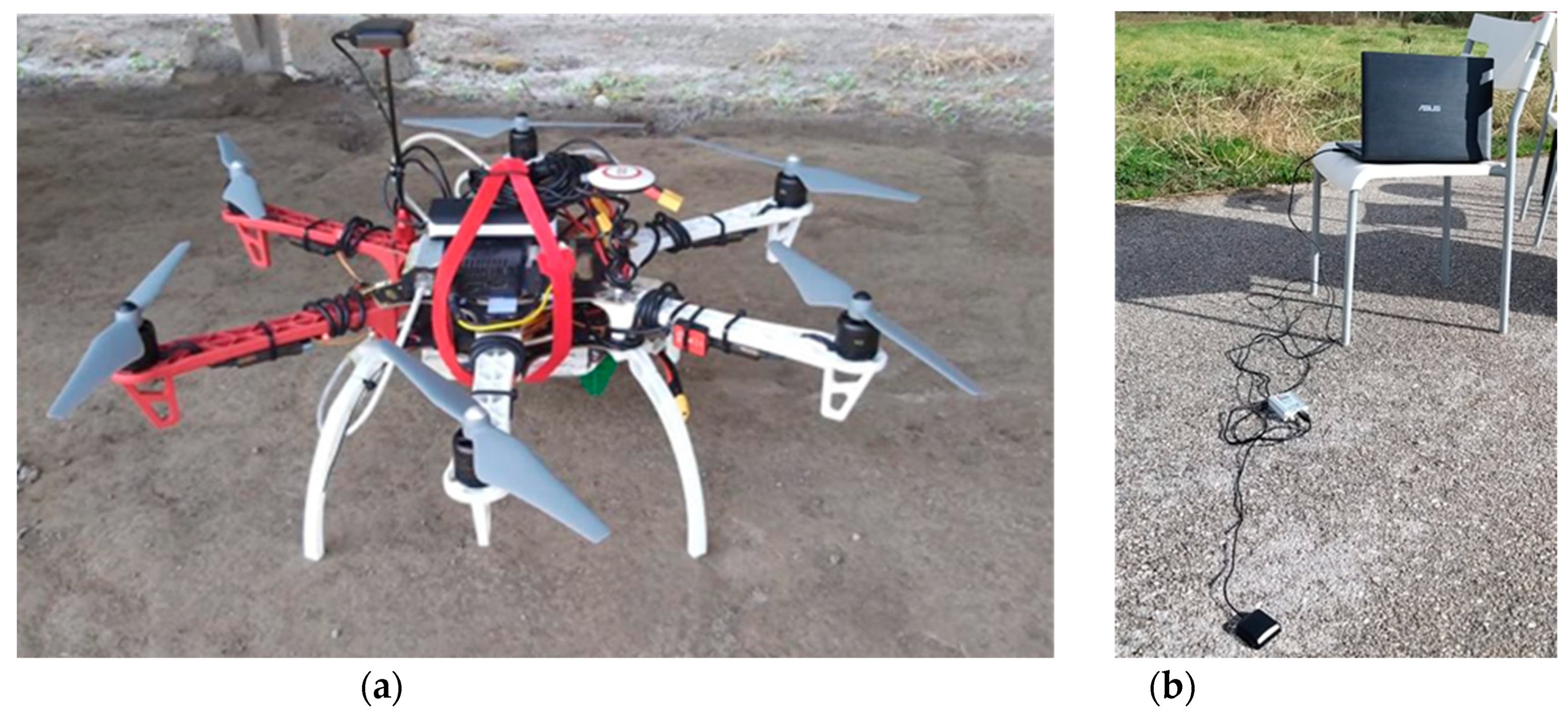
• Small M-UAV platform: DJI F550 hexacopter able to fly at very low speeds (about 1 m/s), thus ensuring a small spatial sampling step and the ability to take-off and land from a very small area;
• Radar system: Pulson P440 radar is a light and compact time-domain device transmitting ultra-wideband pulses (about 1.7 GHz bandwidth centered at the carrier frequency of 3.95 GHz) with a low power consumption [25]. The radar system is mounted rigidly on the UAV body (strapdown installation) and no gimbal is adopted. The limited altitude dynamics experienced during flights (very low ground speed and wind speed conditions resulting in small and almost constant roll/pitch angles), the relatively large radar antenna lobes and the limited baseline between the radar antenna and the drone center of mass are such that altitude/pointing knowledge does not play a significant role;
• GPS receivers/antennas: two single-frequency Ublox LEA-6T devices are chosen, one mounted onboard the UAV and the other one used as a ground-based station. Both are connected to an active patch antenna. The antenna is directly placed on the ground (Figure 1b) in order to get from CDGPS a direct estimate of the height above ground for the antenna mounted on the drone;
• CPU controller: Linux-based Odroid XU4 is devoted to managing the data acquisition for both radar system and onboard GPS receiver, while assuring their time synchronization.

The possibility to estimate the trajectory of the UAV platform depends on the quality of the embarked navigation sensors. By using a standalone onboard GPS receiver, the achievable absolute positioning accuracy is given into a global reference frame, such as WGS84 (World Geodetic System 1984), and is defined according to the specifications provided by the US Department of Defense [26]. Absolute GPS localization errors are estimated as the product of the User Equivalent Range Error (UERE), which is the effective accuracy of the localization errors along the pseudo-range direction, the Horizontal Dilution of Precision (HDOP) and Vertical Dilution of Precision (VDOP). These latter are dimensionless quantities expressing the effect of satellites-receiver geometry. Representative values of UERE, HDOP and VDOP, for good GPS visibility conditions, are, respectively, 3.5 m and 6.6 m [27].

When reasonably short time flights are considered, several error sources (i.e., broadcast clock, broadcast ephemeris, group delay, ionospheric delay and tropospheric delay) are strongly correlated both in space and time [20] and introduce a positioning error, which is an almost constant but unknown bias. In addition, the use of a proper processing strategy, such as carrier-smoothing [20], allows a reduction of the measurement noise [28], thus improving the standalone GPS performance.

As shown in [17], in the frame of radar imaging, it is important to have accurate knowledge of the relative positions of the UAV radar system with respect to the investigated spatial region. Therefore, the constant and unknown bias affecting the horizontal positions provided by a standalone GPS does not play any role in focusing the targets (which, however, will not be reliably localized in the WGS84 reference system), whereas the bias occurring into the vertical position (UAV height) may prejudice satisfactory radar imaging performance.

In this paper, we exploit a strategy based on the use of a CDGPS, which is a method for improving the positioning or timing performance of GPS by exploiting at least one motionless GPS receiver working as a reference station. Here, the CDGPS method is implemented by using two GPS receivers (one mounted onboard the UAV and the other one used at reference ground station), which store the data into a local hard drive.

Each receiver collects single-frequency observables, which is a pseudo-range and a carrier-phase measure for any tracked GPS satellite. It is well-known that carrier-phase measures show significantly reduced measurement noise (in the order of 1/100 of signal wavelength, i.e., mm scale) with respect to pseudo-range ones, but ambiguities appear, so carrier-phase are biased measurements [28,29]. If one is able to resolve the ambiguity, very high accuracy positioning is enabled. This can be achieved by differential techniques, i.e., CDGPS, where differences between the measurements collected by two relatively close receivers are computed. Such differential measures are not affected by common errors between the receivers, due to ionosphere, troposphere and clock errors, so suitable processing is implemented to filter out pseudo-range noise thus deriving an estimate of carrier-phase ambiguities. If a connection through a radio link is established between the UAV and the ground station, CDGPS processing can be performed in real-time, which is defined as “Real-Time Kinematic” (RTK). Offline CDGPS processing is, instead, used in this work, which is typically referred to as “Post-Processing Kinematic” (PPK).

Depending on the working environment, platform dynamics and receiver quality, two different types of CDGPS solutions can be obtained, i.e., fixed or float solutions [30]. The former is the most accurate one, being able to guarantee up to sub-cm accuracy in the determination of the relative position between the receivers, exploiting the property of carrier-phase ambiguities to become, under suitable measurement combinations and for properly designed receivers, integer numbers. The fixed solution can be robustly generated by processing multi-frequency GPS data and can be obtained, although with reduced time availability, by using single-frequency receivers, which typically rely on the float solution, i.e., they consider carrier-phase ambiguities as real numbers. This is the case of the presented system architecture. Hence, for most of the time epochs, a realistic estimate of the carrier-phase ambiguities can be robustly generated by the adopted single-frequency receivers and the achieved accuracy thus degrades to the order of 10 cm. The error is reduced to a very few cm when fixed solutions are available.

Herein, CDGPS processing is carried out by using the open-source software RTKlib [21]. In particular, the post-processing analysis tool RTKPOST is used, which inputs RINEX observation data and navigation message files (from GPS, GLONASS, Galileo, QZSS, BeiDou and SBAS), and can compute the positioning solutions by various processing modes (such as Single-Point, DGPS/DGNSS, Kinematic, Static, PPP-Kinematic and PPP-Static). In this regard, the “Kinematic” positioning mode is chosen, which corresponds to PPK, with integer ambiguity resolution set to “Fix and hold”. RTKPOST outputs the E/N/U coordinates of the flying receiver with respect to the base-station, together with a flag relevant to the solution type (float/fixed). This flag, and the processing residuals, can be used as an estimate of the achieved positioning accuracy.

3. Radar Signal Processing

This section describes the signal processing strategy adopted to process the data collected by the radar system. The various stages of the data processing are summarized in the block diagram of Figure 2. According to this scheme, the input information is the raw radargram (B-scan) collected by the radar, which represents the received radar signal collected at each measurement position (along the flight path) versus the fast-time (i.e., the wave travel time). The final output of the reconstruction procedure is a focused and easily interpretable image depicting the scene under test.

As a first stage of the overall reconstruction procedure, a time-domain pre-processing of the radargram is performed by applying the following operations [31,32,33]:

• Zero-timing;
• Background removal;
• Time-gating.

The zero-timing consists of setting the starting instant of the fast-time axis in such a way that the range of the signal reflected by the air–soil interface at the first measurement point of the flight trajectory is coincident with the UAV flight height estimated by the CDGPS processing.

The background removal is a filtering procedure that allows mitigating the effects of the strong coupling between the transmitting and receiving radar antennas, which is a spatially constant signal. This filter replaces each single radar trace (A-scan) of the radargram with the difference between it and the average of all the traces of the radargram collected along the flight trajectory.

The time-gating procedure selects the interval (along the fast-time) of the radargram, where signals scattered from targets of interest occur. This allows a reduction of environmental clutter and noise effects. Herein, the UAV altitude is exploited to define a suitable time window around the time where reflection of the air–soil interface occurs.

After the time-domain pre-processing stage, each trace in the radargram is transformed into the frequency domain by using the Fast Fourier Transform (FFT) algorithm. Then, the frequency-domain data are processed according to the radar imaging approach detailed in the next subsection.

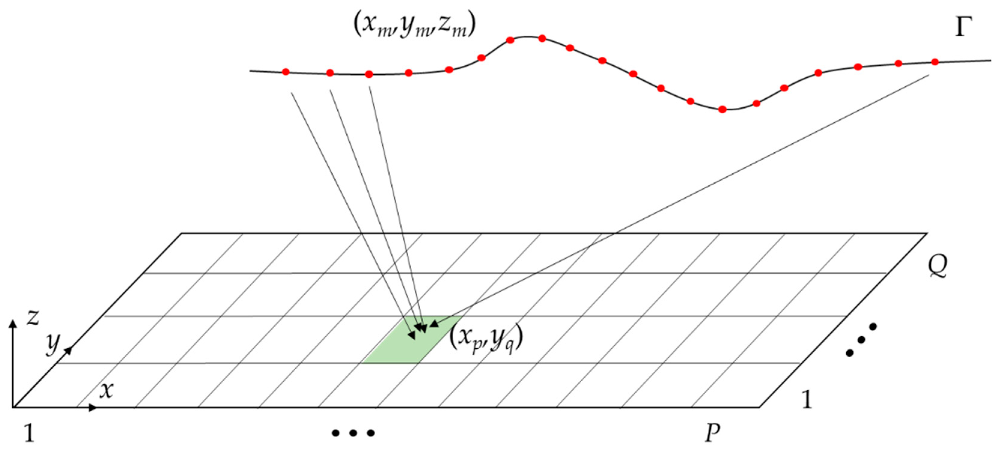
3.1. Radar Imaging Approach

Let us refer to the 3D scenario sketched in Figure 3. The ultra-wideband radar transceiver onboard the UAV illuminates the scene with transmitting and receiving antennas pointed at nadir (down-looking mode), i.e., at a zero incidence angle with respect to the normal to the air–soil interface. The radar can be considered operating in monostatic mode, since transmitting and receiving antennas have negligible offset in terms of the probing wavelength. At each measurement point along the flight trajectory $\mathsf{\Gamma }$, the transceiver records the signals scattered from the targets over the angular frequency range $\Omega =\left[{\omega }_{min},{\omega }_{max}\right]$. Therefore, multimonostatic and multifrequency data are collected.

The trajectory Γ has an arbitrary shape in space and each measurement point is described by the position vector ${\mathit{r}}_{\mathit{m}}=x_m\widehat{x}+y_m\widehat{y}+z_m\widehat{z}$. The targets are supposed to be located into the planar investigation domain D, which is coincident with the air–soil interface assumed at $z=0$. The time dependence $e^{j\omega t}$ is assumed and dropped.

The radar signal model is based on the following assumptions: (i) the antennas have a broad radiation pattern; (ii) the targets are in the far-field region with respect to the radar antennas; (iii) a linear model of the scattering phenomenon is assumed, hence the mutual interactions between the targets are neglected [22]. Accordingly, the scattered signal at each measurement point ${\mathit{r}}_{\mathit{m}}$ is expressed by the following linear integral equation [16,34]:

$$E_s\left({\mathit{r}}_{\mathit{m}},\omega \right)=I\left(\omega \right)\underset{D}{\overset{}{\iint }}\frac{e^{-j2k_0\left|{\mathit{r}}_{\mathit{m}}-\mathit{r}\right|}}{{\left|{\mathit{r}}_{\mathit{m}}-\mathit{r}\right|}^2}\sigma \left(\mathit{r}\right)d\mathit{r}=ℒ\sigma$$

(1)

where $I\left(\omega \right)$ is the spectrum of the transmitted pulse, $\sigma \left(\mathit{r}\right)$ is the unknown reflectivity function at a point $\mathit{r}=x\widehat{x}+y\widehat{y}$ in $D$, $k_0=\omega /c_0$ is the propagation constant in free-space ($c_0\cong 3·{10}^8\left[\mathrm{m}/\mathrm{s}\right]$ is the speed of light) and $\left|{\mathit{r}}_{\mathit{m}}-\mathit{r}\right|$ is the distance between the measurement point and the generic point of the investigation domain $D$. It is worth noting that the spectrum I(ω) may be assumed unitary within the system bandwidth and therefore, for notation simplicity, it will be omitted.

The linear operator $ℒ$ maps the space of the unknown object function (reflectivity of the scene) into the space of data (measured scattered field). The reflectivity function $\sigma \left(\mathit{r}\right)$ accounts for the difference between the electromagnetic properties of the targets (dielectric permittivity, electrical conductivity) and the free space ones. Accordingly, the targets are searched for as anomalies with respect to the free-space scenario and appear in the “focused image” as the regions where the modulus of the reflectivity function is different from zero.

The radar imaging is faced as the inversion of the linear integral Equation (1) and this is performed by computing the adjoint of the forward scattering operator $ℒ$ [23]:

$$\tilde{\sigma }\left(\mathit{r}\right)={ℒ}^{+}{E}_s={\int }_{\mathsf{\Gamma }}^{}{\displaystyle \underset{\mathsf{\Omega }}{\overset{}{\int }}}{E}_s\left({\mathit{r}}_{\mathit{m}},\omega \right)\frac{e^{j2k_0\left|{\mathit{r}}_{\mathit{m}}-\mathit{r}\right|}}{{\left|{\mathit{r}}_{\mathit{m}}-\mathit{r}\right|}^2}d{\mathit{r}}_{\mathit{m}}d\omega$$

(2)

where ${ℒ}^{+}$ is the adjoint operator of $ℒ$.

The adjoint inversion scheme given by Equation (2) is also referred as frequency-domain back-projection [35], since the measured signal is back projected to the point where it is generated and the image is formed as the coherent summation of these contributions.

The numerical implementation of the inversion is performed by discretizing Equation (2) by applying the Method of Moments [36]. The scattered field is discretized by $M\times N$ data, where $M$ is the number of measurement points $\left(x_m,y_m,z_m\right)$, $m=1,2\dots ,M$ and $N$ is the number of angular frequencies ${\omega }_n$, $n=1,2\dots N$ sampling the work frequency bandwidth $\Omega$. The domain $D$ is discretized by $P\times Q$ pixels $\left(x_p,y_q\right)$, where $p=1,2\dots P$, and $=1,2\dots Q$ (see Figure 4). After removing unessential constants, the inversion scheme in Equation (2) is rewritten in discrete form as:

$$\tilde{\sigma }(x_p,y_q)={\displaystyle \sum _{m=1}^M\sum _{n=1}^N}{E}_s(x_m,y_m,z_m,{\omega }_m)\frac{e^{\frac{j2{\omega }_m}{c_0}\sqrt{{(x_p-x_m)}^2+{(y_q-y_m)}^2+z_m^2}}}{{(x_p-x_m)}^2+{(y_q-y_m)}^2+z_m^2}\begin{array}{c}p=1\dots P,\\ q=1\dots Q\end{array}$$

(3)

According to the assumption of antennas having a broad radiation pattern, Equation (3) sums coherently the multi-frequency data collected along the whole trajectory $\mathsf{\Gamma }$ for each pixel in $D$. Therefore, the radar image is obtained by computing Equation (3) for all pixels in $D$ and plotting the magnitude of the retrieved reflectivity values normalized with respect to their maximum value.

In this process, the precise measurement positions of the UAV obtained with the CDGPS processing are considered. The exploitation of the positioning information allows accurate images, as already pointed out in the airborne radar imaging context [24,37].

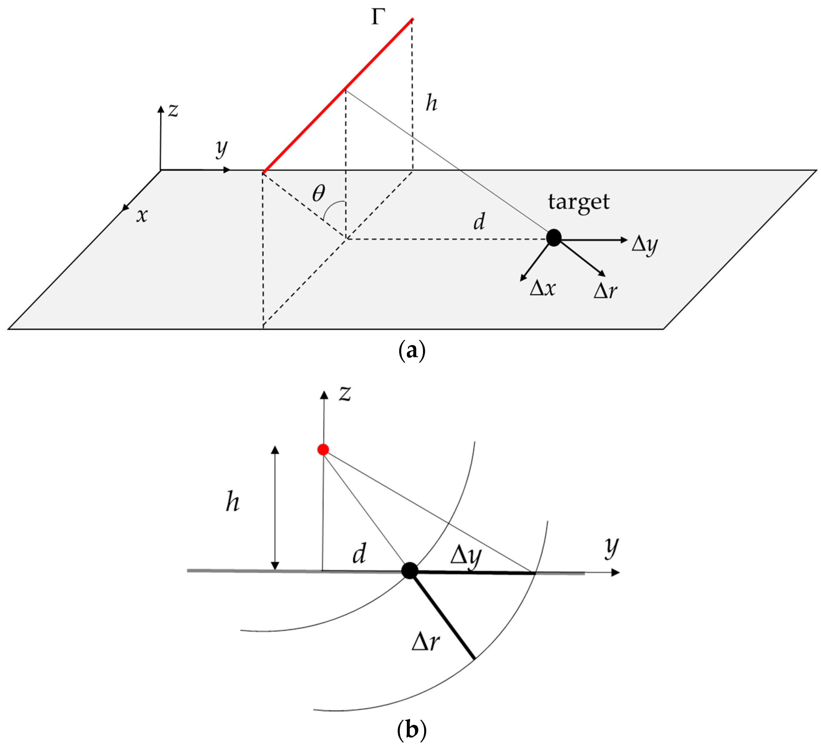
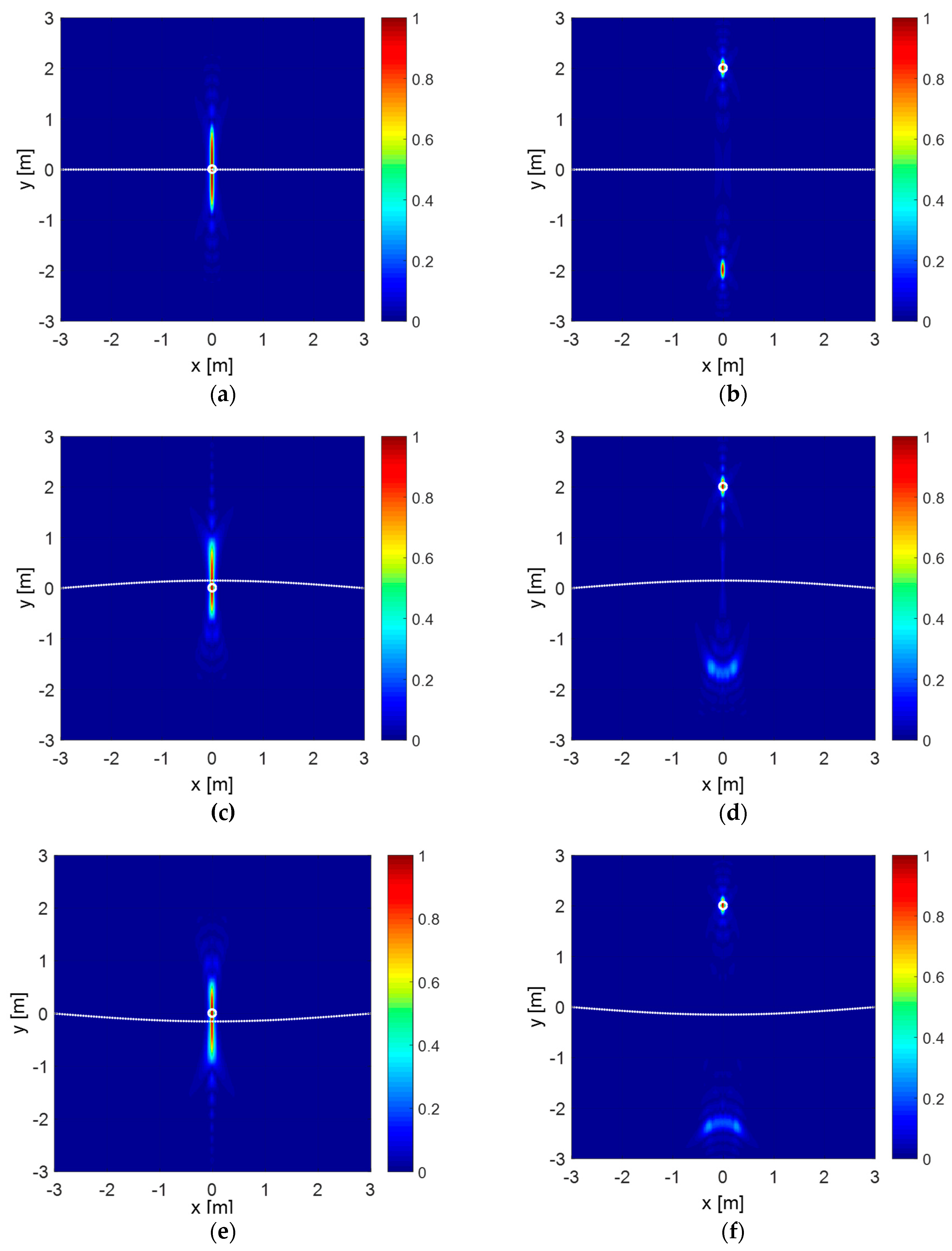
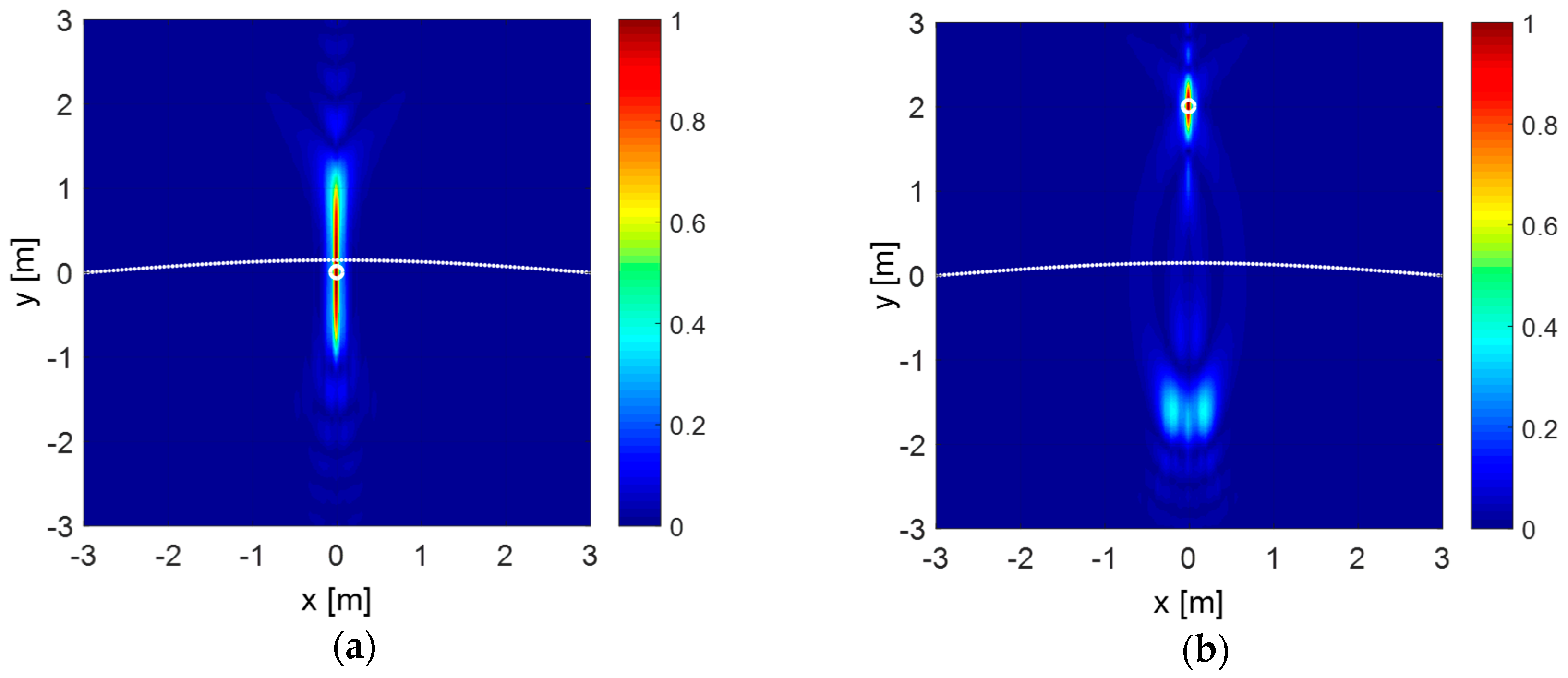
3.2. Resolution Analysis

This subsection aims at investigating the spatial resolution limits of the proposed M-UAV radar imaging system. The analysis covers the effect of the measurement parameters on the resolution limits in the image plane $D$. To achieve this goal, we compute the point spread function (PSF) of the system, i.e., the reconstruction of a point-like target [23]. For a point-like target located at ${\mathit{r}}_{\mathit{t}}=x_t\widehat{x}+y_t\widehat{y}$ and having unitary reflectivity, the related scattered field is expressed, according to Equation (1), as:

$$E_s\left({\mathit{r}}_{\mathit{m}},\omega \right)=\frac{e^{-j2k_0\left|{\mathit{r}}_{\mathit{m}}-{\mathit{r}}_{\mathit{t}}\right|}}{{\left|{\mathit{r}}_{\mathit{m}}-{\mathit{r}}_{\mathit{t}}\right|}^2}$$

(4)

After plugging Equation (4) in the adjoint inversion formula Equation (2), we get the following expression for the PSF

$$\mathrm{PSF}\left(\mathit{r};{\mathit{r}}_{\mathit{t}}\right)={\int }_{\mathsf{\Gamma }}^{}{\displaystyle \underset{\Omega }{\overset{}{\int }}}\frac{e^{-j2k_0\left(\left|{\mathit{r}}_m-{\mathit{r}}_{\mathit{t}}\right|-\left|{\mathit{r}}_m-\mathit{r}\right|\right)}}{{\left|{\mathit{r}}_m-{\mathit{r}}_{\mathit{t}}\right|}^2{\left|{\mathit{r}}_m-\mathit{r}\right|}^2}d{\mathit{r}}_{m}d\omega$$

(5)

allowing the evaluation of the resolution as a function of the system parameters and the flight trajectory. Hence, Equation (5) is useful, on one hand, for planning the measurement campaign according to the requirements of the applicative context of interest and, on the other side, for investigating how deviations, with respect to the nominal flight path, affect the achievable imaging performance.

Before proceeding further, it is worth recalling the resolution formulas holding for an ideal rectilinear flight path. These formulas provide useful insight into radar imaging also under non-ideal motion and allow foreseeing, at least in a qualitative way, the effect of the main measurement parameters.

Let us consider the geometry sketched in Figure 5, where the UAV moves at a fixed height h following a rectilinear trajectory directed along the x-axis. The along-track resolution ${\Delta }_x$ is determined by the central frequency $f_c$ of the radar and the maximum view angle $\theta$ fixed by half-length of the synthetic aperture [32]:

$${\Delta }_x=\frac{c_0}{4f_c\sin \theta }$$

(6)

that in the small angle approximation rewrites as [38]:

$${\Delta }_x=\frac{c_0}{4f_c\theta }$$

(7)

The range resolution is related to the radar system bandwidth B by the classical formula [39]:

$${\Delta }_r=\frac{c_0}{2B}$$

(8)

The across-track resolution ${\Delta }_y$ is evaluated from the projection of the 3D target reconstruction over the image plane (see Figure 5b). If $r$ denotes the target range with respect to the antenna, then the 3D target reconstruction is the cylindrical shell having its axis coincident with the measurement line and its inner and outer radius equal to $r-{\Delta }_r$ and $r+{\Delta }_r$, respectively. Note that only a part of the shell is shown in Figure 5b, for sake of clarity. The across-track resolution ${\Delta }_y$ is calculated as the intersection of the cylindrical shell with the image plane $z=0$ and is given by

$${\Delta }_y=\sqrt{d^2+{\Delta }_r^2+2{\Delta }_r\sqrt{h^2+d^2}}-d$$

(9)

where $d$ is the across-track distance between the fight trajectory and the target (see Figure 5a,b). According to Equation (9), the across-track resolution gets worse when the UAV flies at a higher altitude $h$ and, when the target is illuminated at nadir ($d=0$), it turns out that:

$${\Delta }_y={\Delta }_r\sqrt{1+\frac{2h}{{\Delta }_r}}$$

(10)

i.e., the across-track resolution is finite and larger than the range resolution ${\Delta }_r$.

Equation (9) also reveals that, for a fixed value of $h$ and ${\Delta }_r$, ${\Delta }_y$ improves as long as the target moves away from the measurement line. Most notably, the asymptotic value of the across-track resolution is found as $d$ approaches to infinity:

$${\Delta }_y=\underset{d\to \infty }{\lim }\sqrt{d^2+{\Delta }_r^2+2{\Delta }_r\sqrt{h^2+d^2}}-d={\Delta }_r$$

(11)

Based on the results in the Equations (10) and (11), the following inequality holds:

$${\Delta }_r\le {\Delta }_y\le {\Delta }_r\sqrt{1+\frac{2h}{{\Delta }_r}}$$

(12)

Note that if the system bandwidth $B$ goes to zero, the range resolution ${\Delta }_r$ becomes infinite and it is no longer possible to resolve targets along the direction perpendicular to the track, as already noticed in [24].

Figure 6 depicts the across-track resolution ${\Delta }_y$ as a function of the target offset $d$ and the flight altitude $h$. The contour plot has been produced by applying Equation (9) and considering the bandwidth of the radar system (i.e., $B=1.7\mathrm{GHz}$) introduced in Section 2.

As previously pointed out, the resolution degrades when increasing the flight altitude $h$ for a fixed value of $d$ or when reducing $d$ for a fixed value of $h$.

Figure 7 provides an example of the PSF computed according to Equation (5) by considering an investigation domain $D=\left[-3,3\right]\times \left[-3,3\right]m^2$, which is discretized by square image pixels with size $0.01$ m, and two different values of the target offset $d$ (i.e., $d=0$ m and $d=2$ m). The scattered field data are sampled evenly with $0.01$ m step along the trajectory $\mathsf{\Gamma }$ at a flight altitude $h=5$ m.

Figure 7a,b reports the PSF reconstruction for the case of a rectilinear trajectory covering the interval $\left[-3,3\right]$ along $x$.

Figure 7c,f considers the effect of a non-rectilinear UAV flight trajectory; specifically, the x-directed rectilinear trajectory of Figure 7a,b is perturbed in the $x-y$ plane and modified in accordance with the co-sinusoidal function

$$y=\pm 0.15\cos \left(\frac{\pi x}{12}\right)$$

(13)

Equation (13) defines a curved trajectory over the interval $\left[-3,3\right]$ m with a maximum deviation of $0.15$ m along $y$ with respect to the rectilinear trajectory.

Figure 7a,b shows that a focused spot along and across the track is obtained in correspondence of the target position and the along-track resolution does not change when the target is located at the radar nadir ($d=0$ m) or at the point $\left(0,2\right)$ m. Conversely, the across-track resolution improves when the target is far from the nadir, as predicted by Equation (9). However, in this latter case, a false target appears at the specular position with respect to the flight trajectory, i.e., at $\left(0,-2\right)$ m. This phenomenon is the so-called left–right ambiguity [40] and is due to the radar’s inability to discriminate left $(y>0)$ and right $(y<0)$ targets located at the same distance with respect to the measurement line.

In addition, Figure 7c,f shows that, as expected, even with a slight trajectory deviation with respect to the rectilinear path, the PSF is no longer symmetric with respect to the trajectory. Most notably, when the target is placed at $\left(0,2\right)$ m (see Figure 7d,f), the false target due to the left–right ambiguity appears distorted and with a lower intensity, with respect to Figure 7b. Indeed, when the trajectory is not rigorously rectilinear, the left and right targets are in some way discriminated by the radar because their echoes have different propagation delays at each measurement point. However, the beneficial effect provided by the trajectory curvature in mitigating the false target becomes less relevant when the flight altitude $h$ increases, since left and right targets produce scattering signals with “more similar” propagation delays. This statement is corroborated by the images in Figure 8a,b, which are analogous to Figure 7c,d but for the altitude that is $h=10$ m. As expected, by increasing flight altitude, the resolution across-track degrades regardless of the position of the target and the left–right ambiguity problem turns out to be more evident. The amplitude of the false target seen in Figure 8b is, indeed, stronger compared to the one observed in Figure 7d,f.

The along- and across-track resolution values referred to the considered numerical examples are summarized in

Table 1. Along- and across-track resolution values.

	Along-Track Resolution (m)	Across-Track Resolution (m)
Rectilinear path, target offset $d=0$ m, flight altitude $h=5$ m	0.04	0.95
Rectilinear path, target offset $d=2$ m, flight altitude $h=5$ m	0.04	0.25
Path $y=0.15\cos \left(\frac{\pi x}{12}\right)$, target offset $d=0$ m, flight altitude $h=5$ m	0.04	0.95
Path $y=0.15\cos \left(\frac{\pi x}{12}\right)$, target offset $d=2$ m, flight altitude $h=5$ m	0.04	0.25
Path $y=-0.15\cos \left(\frac{\pi x}{12}\right)$, target offset $d=0$ m, flight altitude $h=5$ m	0.04	0.95
Path $y=-0.15\cos \left(\frac{\pi x}{12}\right)$, target offset $d=2$ m, flight altitude $h=5$ m	0.04	0.25
Path $y=0.15\cos \left(\frac{\pi x}{12}\right)$, target offset $d=0$ m, flight altitude $h=10$ m	0.07	1.30
Path $y=0.15\cos \left(\frac{\pi x}{12}\right)$, target offset $d=2$ m, flight altitude $h=10$ m	0.07	0.47

.

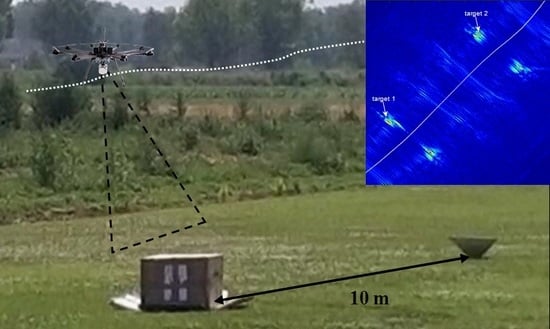
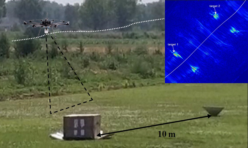
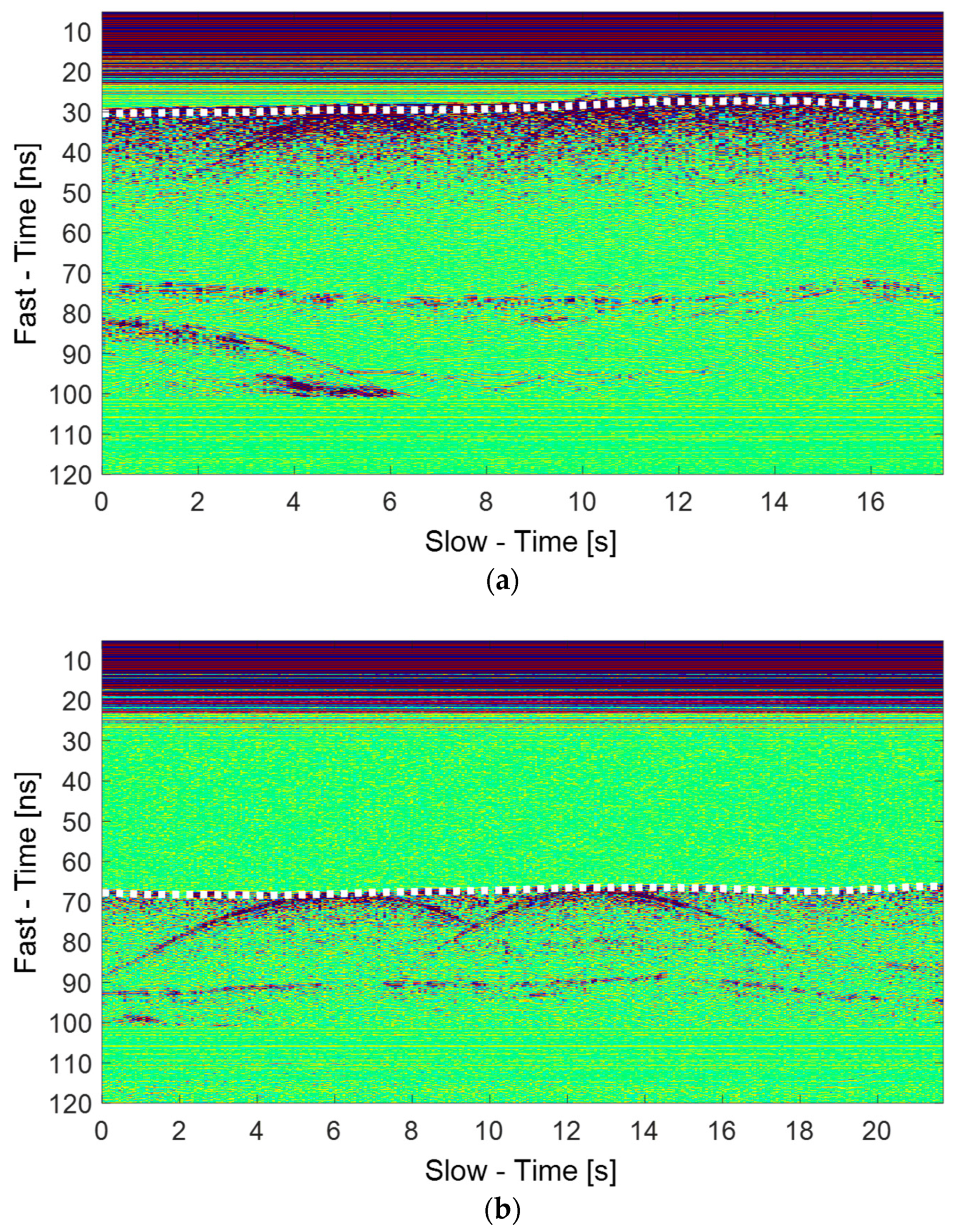
4. Experimental Results

The M-UAV radar imaging system has been experimentally tested at an authorized site for amateur UAV testing flights in Acerra, Naples, Italy. The experiment aimed at testing the ability of the CDGPS technique to estimate the UAV position with the accuracy required for target imaging and, thus, to verify the capability of the overall radar imaging system. The experiment was carried out during a sunny day with a weak wind state. Two metallic trihedral corner reflectors, having a size $D=0.40\mathrm{m}\times 0.40\mathrm{m}\times 0.57\mathrm{m}$ and referred as Target 1 and Target 2, were used as on-ground targets placed at a relative distance of $10\mathrm{m}$ one from the other along the flight direction; one of them (i.e., Target 2) was covered with a cardboard box (see Figure 9).

The UAV was manually piloted and two surveys at different altitudes, in the following referred to as Track 1 and Track 2, were carried out. Both tracks were performed on the same scenario by positioning the UAV nearly at the same starting point $\left(x,y\right)$. Track 1 had a duration of $17.5$ s and covered a path $31.4$ m long at an average altitude $h=4$ m; along this track, data were gathered at $251$ unevenly spaced measurement points. Track 2 had a duration of $21.7$ s and covered a $33$ m long path at an average altitude $h=10$ m; along this track, data were gathered at $331$ unevenly spaced measurement points. The radar parameters set for the data acquisition are summarized in

Table 2. Radar system parameters.

Parameters	Specification
Carrier Frequency	3.95 GHz
Frequency Band	1.7 GHz
Maximum Emitted Power	–13 dBm
Maximum Dynamic Range	75 dB
Pulse Repetition Frequency	14.28 Hz
Received Signal Sampling Frequency	16 GHz

. Note that we considered flight altitude values in the range 5–10 m to operate with a suitable signal-to-noise ratio. Indeed, a major constraint in our system is the limited transmit power of the radar, whose maximum level is declared to be approximately –13 dBm by the manufacturer.

The raw radargrams, i.e., the data collected during the two surveys, are depicted in Figure 10a,b while the filtered radargrams (after the time domain pre-processing stage) are given in Figure 11a,b. It is worth pointing out that the horizontal axis shows the slow-time, i.e., the duration of the flight in seconds, while the vertical axis is the fast-time, i.e., the observation time window during which the data are gathered for each radar position, once that the time-zero correction has been performed. The fast-time is expressed in nanoseconds. The white dotted line represents the air/soil interface achieved by converting the variable UAV flight altitude $h$ estimated by the CDGPS into an equivalent travel time $t_h$ by using the formula $t_h=2h/c_0$.

From Figure 10 and Figure 11, one can observe that the CDGPS provides an accurate estimation of the flight altitudes and the targets’ responses are visible as hyperbolas whose apex occurs at the fast-time where nadir surface reflection is observed. Moreover, Figure 10a,b shows that clutter signals, due to metallic awnings located on the entry side of the flight site, appear at fast-times greater than 70 ns in Figure 10a and 90 ns in Figure 10b. These undesired signals, as well as the mutual coupling between transmitting and receiving antennas, are removed by a time-domain pre-processing (see Figure 11a,b). The filtered radargrams have been obtained by performing the background removal and setting as fast-time gating window the portion occurring 6 ns before and 24 ns after the air–soil interface response seen at nadir. The filtered data have been transformed into the frequency domain by sampling the radar bandwidth [3.1, 4.8] GHz into 341 evenly spaced frequency samples and have been processed according to the inversion procedure described in Section 3.1.

Before showing the focused radar images, we provide quantitative data about the positioning accuracy of the UAV. Specifically,

Table 3. Maximum errors of the CDGPS technique.

Errors (cm)	x	y	z
Track 1	4.3	4.6	9.4
Track 2	0.6	0.8	1.5

summarizes the maximum positioning errors achieved with the CDGPS technique along Tracks 1 and 2. These errors are the standard deviations provided by the RTKlib tool, which measure the positioning errors along the three coordinate axes based on a priori error models and error parameters [21]. The maximum errors in the horizontal plane are always smaller than the error along z, which is 9.4 cm in the worst case (Track 2).

The focused images of the surveyed scenario are depicted in Figure 12a,b for Track 1 and Track 2, respectively. These images have been obtained by considering a square planar investigation domain $D$ at $z=0$ m, whose origin corresponds to the starting point of the UAV tracks into the x–y plane and whose side is 18 m. The domain $D$ has been evenly discretized by pixels having side $0.01$ m.

In Figure 12a,b, the dotted white line represents the M-UAV trajectory as estimated by the CDGPS and projected onto the investigated domain. According to the analysis presented in Section 3.2, Figure 12a shows that when the targets are illuminated at nadir, i.e., when the distance $d$ approaches to zero, single spots appear and no ambiguities occur. Conversely, false targets due to the left–right ambiguity problem appear when the UAV flight path does not cover the targets (see Figure 12b). However, coherently with the PSFs shown in Figure 8b, the false targets appear slightly distorted and with lower intensity compared to the real target reconstructions owing to the trajectory curvature. As a result, it is possible to discriminate the actual targets from the ambiguous ones.

Table 4. Along- and across-track resolution values.

		Experimental Along-Track Resolution (m)	Theoretical Along-Track Resolution (m)	Experimental Across-Track Resolution (m)	Theoretical Across-Track Resolution (m)
Track 11	Target 1	0.05	0.02	1.15	0.85
	Target 2	0.04	0.02	0.99	0.85
Track 22	Target 1	0.07	0.03	0.51	0.41
	Target 2	0.09	0.03	0.50	0.41

¹$h=4m,d=0m$; ²$h=10m,d=2m$

reports the experimental along- and across-track resolution values as estimated by Figure 12a,b for both targets. For comparison, the table reports the theoretical resolution values referred to a rectilinear flight path at the average altitudes h = 4 m and h = 10 m. The experimental and theoretical resolution values are quite consistent. Notably, the experimental along-track resolution decreases slightly when the flight altitude increases and the target offset $d$ is not null, while the across-track one improves when d increases. It is worth pointing out that the corner reflectors emphasize the radar echoes but they are not actually ideal point targets. Consequently, some discrepancies on resolution values are expected and this outcome is confirmed by the comparison between the experimental and theoretical data reported in Table 4.

5. Discussion

This work deals with a feasibility study on small UAV-based radar imaging when the scene under investigation is probed with a single measurement line and the imaging domain is a plane at a fixed altitude. The considered acquisition geometry is the simplest one and its achievable imaging capabilities have been studied in Section 4. Regarding the along-track resolution, this parameter is influenced by the maximum illumination angle, which in turn depends on the flight altitude and the length of the synthetic aperture. The flight height and the horizontal displacement between the target and the UAV, instead, influence the across-track resolution. Targets far from the radar nadir are generally better resolved across-track than those seen at nadir; however, an inherent limitation in the imaging arises due to the left–right ambiguity problem. This phenomenon is partially mitigated in the presence of horizontal deviations of the UAV with respect to the ideal rectilinear trajectory. Additionally, flying at a higher altitude can be convenient to enlarge the area of coverage but such choice generally produces a worsening of the spatial resolution both along- and across-track.

A further point worth to be discussed concerns the inability of the present imaging configuration to provide unambiguous and high-resolution 3D target reconstructions. To clarify this point, it is useful to refer to Figure 13 showing how the reconstruction of the target changes when the image plane is not the correct one. In particular, in Figure 13, we show how a point target located on the plane $D_0$ at z = 0 is imaged on three planes $D_0$, $D_1$, $D_2$ placed at different altitudes, i.e., z = 0, $z=z_1$, and $z=z_2$.

If the image plane coincides with the plane where the target is located, i.e., $D_0$, the target is reconstructed at the correct position. When the image plane is different from $D_0$, i.e., $D_1$ or $D_2,$ due to the cylindrical symmetry of the 3D target reconstruction, the target is imaged at a position different from the true one in the considered plane. The position of the reconstructed target is equal to the intersection point between the 3D reconstruction and the plane where the imaging is carried out. Furthermore, due to the left–right ambiguity, two specular targets appear on both sides of the track (see red rectangles on planes $D_1$ or $D_2$). The spatial offset $\tilde{d}$ in the x–y plane between the true target and the reconstructed one for an image plane at a height $z$ can be derived after straightforward geometrical considerations and is given by

$$\tilde{d}=\sqrt{d^2+2hz-z^2}-d.$$

(14)

This last formula holds also in the more general case when the target is not illuminated at the radar nadir, as in Figure 13, and $d$ is the horizontal distance between the target and the track.

The geometry in Figure 13 also reveals that the target can be detected (but not correctly localized) when the imaging plane is placed at a higher elevation with respect to the target. Indeed, in this case, it is still possible to find two intersection points between the 3D target reconstruction and the image plane. Conversely, the target cannot be identified at all when it is located above the image plane since this last no longer intersects the 3D target reconstruction.

A numerical example showing the effect of the elevation of the image plane is presented in the case of a multi-target scenario. Specifically, the example refers to the rectilinear trajectory and simulation parameters already considered in Section 3.2. The scene comprises three point targets T1, T2, T3 aligned along the flight track and located at coordinates: (−2, 0, 0) m, (0, 0, 0.2) m, (2, 0, 0.4) m. The reconstructions results achieved on three images planes at z = 0, 0.2 and 0.4 m are displayed in Figure 14a–c, respectively. As can be observed in Figure 14a, only the target T1 is imaged and correctly localized in the plane z = 0 m while the targets T2 and T3 are not detected because they are located above the image plane. When the image plane is fixed at z = 0.2 m, the target T2 is the only one to be correctly localized while T1 is imaged a different location with a spatial offset with respect to the true position. The target T3 is still not detectable because its elevation is greater than the height of the image plane. Finally, Figure 14c shows the reconstruction in the plane z = 0.4m. In this case, all targets are detected but only T3 is correctly localized.

Table 5. Estimated and true target positions for different imaging planes.

	True Target Position	Retrieved Target Positions Versus Height of Image Plane
		z = 0 m	z = 0.2 m	z = 0.4 m
T1	(−2, 0, 0) m	(−2, 0, 0) m	(−2, ±1.4, 0.2)	(−2, ±1.99, 0.4) m
T2	(0, 0, 0.2) m	-	(0, 0, 0.2)	(0, ±1.4, 0.4) m
T3	(2, 0, 0.4) m	-	-	(2, 0, 0.4) m

reported below compares the true and reconstructed targets’ positions achieved in each image plane. The maximum of each spot in the images of Figure 14a–c is considered as the estimate of the targets’ positions. Note that the ± sign appears in the presence of the left–right ambiguity problem.

An improvement of the approach in terms of resolution and left–right ambiguity suppression toward a high-resolution 3D imaging can be achieved by collecting wideband scattered field data along multiple (parallel) measurement tracks. A similar measurement configuration has been recently studied in the single-frequency case [24]. The theoretical and experimental assessment of such a configuration in the multifrequency case will be the subject of future research.

As a further upgrade of the radar imaging system, the possibility of using a gimbal, as suggested in [41,42], will be considered to achieve major flexibility in the data acquisition.

6. Conclusions

A proof of concept of a Multicopter Unmanned Aerial Vehicle (M-UAV) radar imaging system has been developed by integrating a miniaturized and commercial radar system onboard a small M-UAV. The imaging system has been equipped with two Global Positioning System (GPS) receivers, the first one located onboard the M-UAV platform, and, the second one used as a ground-based station with the aim of exploiting the Carrier-Phase-Based Differential GPS (CDGPS) technique. This latter allows estimating the 3D M-UAV flight path with centimeter accuracy. Moreover, an advanced imaging approach, based on the adjoint inverse scattering problem, has been adopted to obtain focused images of on surface targets in the case of a single flight track. This approach exploits the 3D M-UAV trajectory estimate provided by the CDGPS into the reconstruction stage.

A theoretical/numerical analysis has been preliminary conducted to evaluate the effect of the overall system and measurement configuration parameters on the imaging system performance. In addition, a proof of concept measurement campaign has been performed. The flight tests have been carried out by manually piloting the UAV at an authorized site for amateur and the experimental results have demonstrated the capability of the system to obtain very good imaging results, comparable to those foreseen with the theoretical analysis. This was possible thanks to the accurate UAV positioning estimation, which means an accurate knowledge of the measurement points, that is a key factor for a reliable focusing of the targets. It is worth noting that, despite the simple and light radar system adopted in this work, the necessity of dealing with high frequency a working band and centimetric probing wavelength (7.5 cm at the frequency of 4 GHz) has made significantly challenging the necessity to have an accurate UAV positioning estimate. This was necessary for a reliable focusing procedure requiring knowledge of the location of the measurement points along the flight trajectory with an accuracy comparable with the probing wavelength.

A final comment is dedicated to future developments. Indeed, to overcome the ambiguity effects caused by the nadir antenna pointing, non-rectilinear trajectory, such as circular or slanting flights are worth being considered. The planning of a measurement campaign involving this kind of flight is the subject of current work. In addition, further flight tests will be conducted to assess the subsurface imaging system capability. Moreover, waypoint following and grid surveys will be exploited to regularly sample the area of interest, and multi-constellation/multi-frequency GNSS will be tested. In this frame, more sophisticated flight/navigation modes and 3D tomographic imaging approaches based on multiple measurement lines will be exploited, in order to open novel remote sensing perspectives in structural monitoring and cultural heritage contexts.

References

1. Everaerts, J. The Use of Unmanned Aerial Vehicles (UAVs) for Remote Sensing and Mapping. Int. Arch. Photogramm. Remote Sens. Spat. Inf. Sci. 2008, 37, 1187–1192. [Google Scholar]
2. Quan, Q. Introduction to Multicopter Design and Control; Springer: Singapore, 2017. [Google Scholar]
3. Colomina, I.; Molina, P. Unmanned Aerial Systems for Photogrammetry and Remote Sensing: A review. ISPRS J. Photogramm. Remote Sens. 2014, 92, 79–97. [Google Scholar] [CrossRef] [Green Version]
4. Yao, H.; Qin, R.; Chen, X. Unmanned Aerial Vehicle for Remote Sensing Applications—A review. Remote Sens. 2019, 11, 1443. [Google Scholar] [CrossRef] [Green Version]
5. Catapano, I.; Di Napoli, R.; Soldovieri, F.; Bavusi, M.; Loperte, A.; Dumoulin, J. Structural Monitoring via Microwave Tomography-Enhanced GPR: The Montagnole test site. J. Geophys. Eng. 2012, 9, 100–107. [Google Scholar] [CrossRef]
6. Oriot, H.; Cantalloube, H. Circular SAR imagery for urban remote sensing. In Proceedings of the 7th European Conference on Synthetic Aperture Radar, Friedrichshafen, Germany, 2–5 June 2008. [Google Scholar]
7. Chao, H.; Cao, Y.; Chen, Y. Autopilots for Small Unmanned Aerial Vehicles: A survey. Int. J. Control Autom. Syst. 2010, 8, 36–44. [Google Scholar] [CrossRef]
8. Massonnet, D.; Souyris, J.C. Imaging with Synthetic Aperture Radar; EPFL Press: Lausanne, Switzerland, 2008. [Google Scholar]
9. Cunliffe, A.M.; Brazier, R.E.; Anderson, K. Ultra-fine grain landscape-scale quantification of dryland vegetation structure with drone-acquired structure-from-motion photogrammetry. Remote Sens. Environ. 2016, 183, 129–143. [Google Scholar] [CrossRef] [Green Version]
10. Li, C.J.; Ling, H. High-resolution, downward-looking radar imaging using a small consumer drone. In Proceedings of the 2016 IEEE International Symposium on Antennas and Propagation (APSURSI), Fajardo, Puerto Rico, 26 June–1 July 2016; pp. 2037–2038. [Google Scholar]
11. Bhardwaj, A.; Sam, L.; Akansha, L.; Martin-Torres, F.J.; Kumar, R. UAVs as remote sensing platform in glaciology: Present applications and future prospects. Remote Sens. Environ. 2016, 175, 196–204. [Google Scholar] [CrossRef]
12. Remy, M.A.; de Macedo, K.A.; Moreira, J.R. The first UAV-based P-and X-band interferometric SAR system. In Proceedings of the 2012 IEEE International Geoscience and Remote Sensing Symposium (IGARSS), Munich, Germany, 22–27 July 2012; pp. 5041–5044. [Google Scholar]
13. Llort, M.; Aguasca, A.; Lopez-Martinez, C.; Martínez-Marin, T. Initial Evaluation of SAR Capabilities in UAV Multicopter Platforms. IEEE J. Sel. Top. Appl. Earth Obs. Remote Sens. 2018, 11, 127–140. [Google Scholar] [CrossRef] [Green Version]
14. Amiri, A.; Tong, K.; Chetty, K. Feasibility study of multi-frequency ground penetrating radar for rotary UAV platforms. In Proceedings of the IET International Conference on Radar Systems, Glasgow, UK, 22–25 October 2012; pp. 1–6. [Google Scholar]
15. Fernández, M.G.; López, Y.Á.; Arboleya, A.A.; Valdés, B.G.; Vaqueiro, Y.R.; Andrés, F.L.H.; García, A.P. Synthetic aperture radar imaging system for landmine detection using a ground penetrating radar on board a unmanned aerial vehicle. IEEE Access 2018, 6, 45100–45112. [Google Scholar] [CrossRef]
16. Soumekh, M. Synthetic Aperture Radar Signal Processing; Wiley: New York, NY, USA, 1999; Volume 7. [Google Scholar]
17. Ludeno, G.; Catapano, I.; Renga, A.; Vetrella, A.; Fasano, G.; Soldovieri, F. Assessment of a micro-UAV system for microwave tomography radar imaging. Remote Sens. Environ. 2018, 212, 90–102. [Google Scholar] [CrossRef]
18. Chao, H.; Gu, Y.; Napolitano, M. A Survey of Optical Flow Techniques for Robotics Navigation Applications. J. Intell. Robot. Syst. 2013, 73, 361–372. [Google Scholar] [CrossRef]
19. Fletcher, I.; Watts, C.; Miller, E.; Rabinkin, D. Minimum entropy autofocus for 3D SAR images from a UAV platform. In Proceedings of the 2016 IEEE Radar Conference (RadarConf), Philadelphia, PA, USA, 2–6 May 2016; pp. 1–5. [Google Scholar]
20. Kaplan, E.; Hegarty, C.J. Understanding GPS–Principles and Applications, 2nd ed.; Artech House: Boston, MA, USA; London, UK, 2006. [Google Scholar]
21. Available online: http://www.rtklib.com/rtklib_document.htm (accessed on 28 February 2020).
22. Chew, W.C. Waves and Fields in Inhomogeneous Media; IEEE Press: Piscataway, NJ, USA, 1995. [Google Scholar]
23. Bertero, M.; Boccacci, P. Introduction to Inverse Problems in Imaging; CRC Press: Boca Raton, FL, USA, 1998. [Google Scholar]
24. Gennarelli, G.; Catapano, I.; Soldovieri, F. Reconstruction capabilities of down-looking airborne GPRs: The single frequency case. IEEE Trans. Comput. Imaging 2017, 3, 917–927. [Google Scholar] [CrossRef]
25. Available online: https://www.humatics.com/products/scholar-radar/ (accessed on 28 February 2020).
26. Standard, G.S.P. Available online: https://trade.ec.europa.eu/tradehelp/standard-gsp (accessed on 28 February 2020).
27. Milbert, D. Dilution of precision revisited. Navigation 2008, 55, 67–81. [Google Scholar] [CrossRef]
28. Farrell, J.A. Aided Navigation: GPS with High Rate Sensors; Mc Graw. Hill: New York, NY, USA, 2–5 June 2008. [Google Scholar]
29. Groves, P.D. Principles of GNSS, Inertial, and Multisensor Integrated Navigation Systems; Artech House: Norwood, MA, USA, 2008. [Google Scholar]
30. Renga, A.; Fasano, G.; Accardo, D.; Grassi, M.; Tancredi, U.; Rufino, G.; Simonetti, A. Navigation facility for high accuracy offline trajectory and attitude estimation in airborne applications. Int. J. Navig. Obs. 2013, 1–13. [Google Scholar] [CrossRef] [Green Version]
31. Daniels, D.J. Ground penetrating radar. In Encyclopedia of RF and Microwave Engineering; John Wiley & Sons: Hoboken, NJ, USA, 2005. [Google Scholar]
32. Persico, R. Introduction to Ground Penetrating Radar: Inverse Scattering and Data Processing; John Wiley & Sons: Hoboken, NJ, USA, 2014. [Google Scholar]
33. Catapano, I.; Gennarelli, G.; Ludeno, G.; Soldovieri, F.; Persico, R. Ground-Penetrating Radar: Operation Principle and Data Processing. Wiley Encycl. Electr. Electron. Eng. 2019, 1–23. [Google Scholar]
34. Balanis, C.A. Advanced Engineering Electromagnetics; John Wiley & Sons: Hoboken, NJ, USA, 1999. [Google Scholar]
35. Solimene, R.; Catapano, I.; Gennarelli, G.; Cuccaro, A.; Dell’Aversano, A.; Soldovieri, F. SAR Imaging Algorithms and some Unconventional Applications: A Unified Mathematical Overview. IEEE Signal Proc. Mag. 2014, 31, 90–98. [Google Scholar] [CrossRef]
36. Harrington, R.F. Field Computation by Moment Methods; Wiley-IEEE Press: Hoboken, NJ, USA, 1993. [Google Scholar]
37. Gennarelli, G.; Catapano, I.; Ludeno, G.; Noviello, C.; Papa, C.; Pica, G.; Soldovieri, F.; Alberti, G. A low frequency airborne GPR System for Wide Area Geophysical Surveys: The Case Study of Morocco Desert. Remote Sens. Environ. 2019, 233, 111409. [Google Scholar] [CrossRef]
38. Scherzer, O. Handbook of Mathematical Methods in Imaging; Springer Science & Business Media: Berlin, Germany, 2010. [Google Scholar]
39. Richards, M.A. Fundamentals of Radar Signal Processing; Tata McGraw-Hill Education: New York, NY, USA, 2005. [Google Scholar]
40. Cheney, M.; Borden, B. Fundamentals of Radar Imaging; Siam: Philadelphia, PA, USA, 2009; Volume 79. [Google Scholar]
41. Gašparović, M.; Jurjević, L. Gimbal influence on the stability of exterior orientation parameters of UAV acquired images. Sensors 2017, 17, 401. [Google Scholar] [CrossRef] [PubMed] [Green Version]
42. Pérez, J.A.; Gonçalves, G.R.; Rangel, J.M.G.; Ortega, P.F. Accuracy and effectiveness of orthophotos obtained from low cost UASs video imagery for traffic accident scenes documentation. Adv. Eng. Softw. 2019, 132, 47–54. [Google Scholar] [CrossRef]
Figure 1. M-UAV radar imaging system: (a) hexacopter with onboard equipment; (b) ground-based GPS station.
Remotesensing 12 00774 g001
Figure 2. Radar signal processing chain.
Remotesensing 12 00774 g002
Figure 3. UAV-borne radar imaging scenario.
Remotesensing 12 00774 g003
Figure 4. Discretization of the radar imaging problem.
Remotesensing 12 00774 g004
Figure 5. Radar imaging with an ideal rectilinear flight path: (a) 3D view; (b) view in the yz plane.
Remotesensing 12 00774 g005
Figure 6. Contour plot of the across-track resolution Δ y versus d and h , expressed in meters, in the case of a rectilinear flight trajectory.
Remotesensing 12 00774 g006
Figure 7. Point spread function (PSF) amplitude for a flight altitude h = 5   m : ideal rectilinear trajectory and point like target with offset: (a) d = 0 m, (b) d = 2 m. Curved trajectory as described by Equation (13) and point-like target located with offset: (c,e) d = 0 m, (d,f) d = 2 m. The white dashed line represents the trajectory and the white circle denotes the target.
Remotesensing 12 00774 g007
Figure 8. PSF amplitude for h = 10 m and a curved trajectory: (a) point like target at d = 0 ; (b) point like target at d = 2 . The white dashed line shows the trajectory; the white circle denotes the target.
Remotesensing 12 00774 g008
Figure 9. The UAV-borne radar imaging scenario.
Remotesensing 12 00774 g009
Figure 10. Raw radargrams: (a) Track 1; (b) Track 2. The white dotted line represents the variable UAV flight altitude h estimated by the Carrier-Phase Differential GPS (CDGPS) and transformed into the equivalent travel time by: t h = 2 h / c 0 .
Remotesensing 12 00774 g010
Figure 11. Filtered radargrams: (a) Track 1; (b) Track 2. The white dotted line represents the variable UAV flight altitude h estimated by the CDGPS and transformed in the equivalent travel time by: t h = 2 h / c 0 .
Remotesensing 12 00774 g011
Figure 12. Focused image of the scenario under test: (a) Track 1; (b) Track 2. The dotted white line represents the flight path as projected onto the investigated domain.
Remotesensing 12 00774 g012
Figure 13. Reconstruction of a point target on image planes at different elevations. The true target (black triangle) is illuminated at the radar nadir and its reconstruction is represented by the red rectangles.
Remotesensing 12 00774 g013
Figure 14. Reconstruction results in a three-target scenario (a) image plane at z = 0 m; (b) image plane at z = 0.2 m; (c) image plane at z = 0.4 m.
Remotesensing 12 00774 g014