Automatic Detection System of Olive Trees Using Improved K-Means Algorithm

Abstract

Olive cultivation over the past few years has spread across Mediterranean countries with Spain being the world’s largest olive producer among them. Because olives are a major part of the economy for such countries keeping records of their tree count and crop yield is of high significance. Manual counting of trees over such large areas is humanly infeasible. To address this problem, we propose an automatic method for the detection and enumeration of olive trees. The algorithm is a multi-step classification system comprising pre-processing, image segmentation, feature extraction, and classification. RGB satellite images were acquired from the Spanish territory and pre-processed to suppress the additive noise. The region of interest was then segmented from the pre-processed images using K-Means segmentation, through which statistical features were extracted and classified. Promising results were achieved for all classifiers, namely Naive Bayesian, Support Vector Machines (SVMs), Random Forest and Multi-Layer Perceptrons (MLPs), at various division ratios of data samples. In a comparison of all the classification algorithms, Random Forest outperformed the rest by an overall accuracy of 97.5% at the division ratio of 70 to 30 for training to testing.

1. Introduction

Olive fruit possesses high agricultural significance, being a major part of the economy for countries such as Spain, Italy, Greece, and Turkey. Today, Spain is the leader of olive production, producing 5,276,899 metric tons of olives on over 2.4 million hectares of dedicated land. Over the last 25 years, consumption of olive oil has increased by 73% and is anticipated to exceed the production by 13% this year [1].

The production and distribution of economically significant crops need to be recorded and maintained for both agriculturists and economists. Manual collection of data over large areas is humanly infeasible, time-consuming, and prone to human error. Advancements in the field of image processing and the availability of very high resolution (VHR) imagery has led to automatic detection and counting [2], which aim to achieve the above-mentioned goal.

Automatic detection of olive trees has remained a challenging topic for researchers. Various basic image pre-processing techniques including image segmentation [3], blob detection [4,5,6], and template matching [7] have been devised for accurate remote detection. Similarly, complex techniques with artificial intelligence enabled [8] and classification-based systems has also been proposed [9,10] to achieve accurate and confident detection results.

Previous methods showed promising results, while leaving room for the application of accurate and heuristic segmentation techniques along with the development of an accurate yet computationally efficient multi-staged olive tree classification system. In addition, these algorithms have been tested over less demanding environments, characterized by fewer ground classes captured over fewer sample images. Our proposed system aims to achieve accurate detection and classification of olive trees in highly diverse environment captured over a large set of aerial images, addressing the limitations in the previous work. It contributes to the domain knowledge by:

• utilizing the heuristic based, improved K-Means clustering algorithm for better segmentation results;
• developing a computationally efficient and robust multi-step based classification model for accurate detection and identification of olive trees; and
• training and testing the proposed system over a large set of diverse images with varying ground information.

The rest of the paper is organized as follows. Section 2 presents the existing literature on olive tree detection followed by the methodology discussed in Section 3. Section 4 covers the experimental setup followed by results in Section 5. Section 6 concludes the paper along with the discussion of future work.

2. Related Literature

2.1. Early 1990s and 2000s

Starting in 1990, Karantzalos and Argialas proposed a blob detection based method to detect olive trees in satellite imagery acquired from Quickbird and IKONOS [5]. In 2000, the Joint Research Centre (JRC) developed a tool called OLICOUNT to count olive trees in grey-scale input image [11]. The tool utilized a combination of techniques such as thresholding, region growing, and morphological operations. Advancements in the tools were made, resulting in OLICOUNT v2 with 16-bit image support [12].

2.2. Late 2000s

Gonzales et al. in 2007 developed a probabilistic model to count the olive trees [7] over the imagery acquired through QUICKBIRD satellite. The probability was calculated for a tree if it was a part of a reticle along with exhibiting the geometrical features such as size, shape, and the angle formed among the trees. The technique resulted in detection accuracy of 98%. In 2009, Arbor Crown Enumerator (ACE), the algorithm proposed by Ionis et al., detected olive trees in multi-spectral imagery [6]. The algorithm utilized the red band thresholding along with the NDVI-based detection method, resulting in an overall estimation error of 1.3%. In the same year, a classification model was proposed by Yakoub et al. to detect olive trees in the agricultural area of Al Jouf, Saudi Arabia acquired by IKONOS-2 [9]. The method utilized a Gaussian Process Classifier (GPC) classifying morphological features of ground data with an overall accuracy of 96%.

2.3. 2010 to Present

In 2010, Garcia et al. proposed multiple methods to detect olive trees from satellite acquired from the SIGPAC viewer of Ministry of Environment and Rural and Marine Affairs, Spain (http://sigpac.mapa.es/fega/visor/) images [3]. Testing samples were formed from the SIGPAC satellite viewer. In one of the methods, they detected olive trees by extracting them as segments formed by K-Means clustering. The results showed an overall omission rate of zero in six samples and a commission rate of one in six. Other methods utilized fuzzy logic, generating a fuzzy number to detect the olive trees using k-neighbor approach [8]. Promising results were obtained from the methodology showing an omission rate of one in six and a commission rate of zero. The results were generated using the value of k as 1 and 2.

In 2011, an object-based classification method was proposed by Jan Peters et al. to detect olive trees from multi-spectral images covering the region of France [10]. The method was comprised of a four-step model: image segmentation, feature extraction, classification, and result mapping. Synergy models were developed at each stage of the technique by combining features from various sensors giving an overall accuracy of 84.3%.

In 2017, Chemin et al. [4] proposed a method to monitor the massive loss of olive trees due to the deadly pathogen, Xylella Fastidiosa over the region of Apuglia, Italy [13]. Multi-spectral images were pre-processed to NDVI followed by segmentation based on Niblack’s thresholding method and Sauvola binarization [14]. Segments falling within defined parameters of size and area were considered to be olive trees, resulting in an overall mean error of 13%. In 2018, Khan et al. [15] proposed a computationally efficient method to detect olive trees over the territory of Spain. They employed basic image processing techniques such as unsharp masking and threshold-based segmentation to detect and count olive trees. Segmented trees were made part of the tree count if lying within the possible size range. The algorithm showed an overall accuracy of 96%.

Related work done in the past years show the proposition of various techniques and methods to detect olive trees. Techniques from simple image segmentation and blob detection to complex methods of classification have been proposed. It has been observed that all previous techniques in the literature showed high accuracy but with a few limitations. Application of simple and efficient threshold-based segmentation techniques along with blob-detection-based methods gave decently accurate results but were highly prone to false positives. Sequential application of the above-mentioned techniques over multi-spectral images enhanced detection accuracy with increase in computational cost. In addition, the respective techniques also showed limitations towards omission and commission errors. When it comes to classification based systems, publicly available datasets with enough images covering diverse cases were not made part of the testing images, leaving room for improvement in the classification results. Our proposed technique focuses on overcoming these shortcomings along with validating it over a diverse dataset in terms of both number of images and ground cover classes.

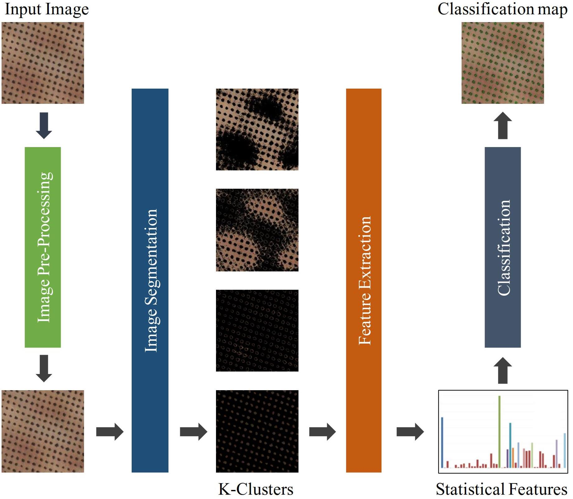
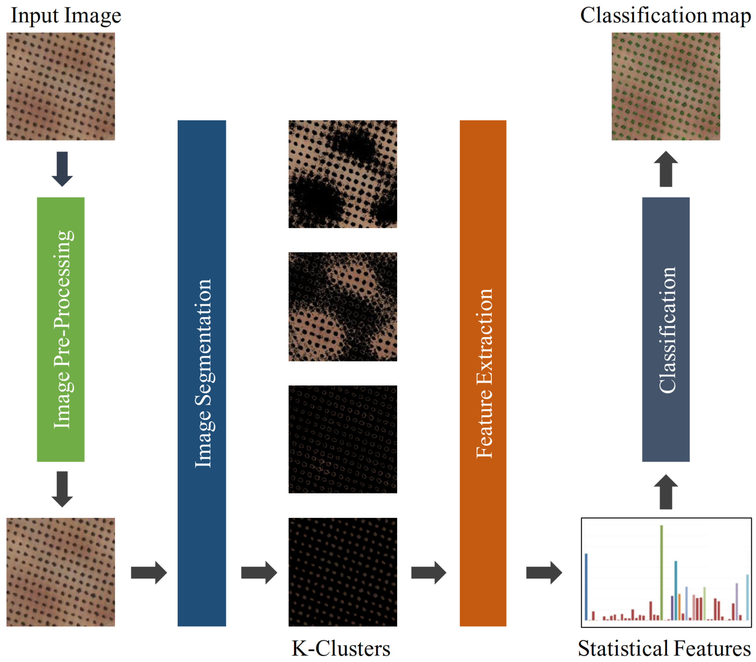
3. Proposed Scheme of Automatic Detection of Olive Trees

In this paper, a method for detecting olive trees in plantation areas using classification is proposed. The aim was to design and develop an olive tree detection algorithm that is accurate in prediction, able to handle many image data, scalable to multi-spectral imagery, and robust in producing accurate results in varying land/tree scenarios in the imagery. The multi-step algorithm utilizes a combination of techniques: pre-processing, segmentation, feature extraction, and classification. The workflow diagram of our proposed system is shown in Figure 1.

3.1. Image Pre-Processing

Image pre-processing is the initial step of our algorithm in which the colored images undergo the noise removal and any other irregularities obscuring the desired information. During the formation of the images, they may encounter errors due to low luminance, motion blur, and mechanical noise added due to optical devices. Input images are pre-processed, removing such errors by smoothing the effect of noise followed by edge enhancement for better results in later stages [16].

3.2. Image Enhancement Using Laplacian of Gaussian (LoG) Filtering

Laplacian filter is used to highlight the regions showing abrupt changes in intensity levels resulting in enhanced edges of the image [17]. Considering the sensitivity of the Laplacian filter to noise, the Gaussian filter is used as a smoothing operator to normalize the noise within the image [18]. The 2D Gaussian is given in Equation (1),

$$G(x,y)=\frac{1}{2\pi {\sigma }^2}{e}^{\left(-\frac{(x^2+y^2)}{2{\sigma }^2}\right)}$$

(1)

where $\sigma$ is the standard deviation. The convolution result of the Gaussian filter with the input image im(x,y) is given in Equation (2) as,

$$L(x,y)=im(x,y)*G(x,y)$$

(2)

where * represents the convolution operator and L(x,y) is the Gaussian scale space representation of the input image im(x,y). The Laplacian is given in Equation (3) as,

$$\begin{array}{c}\hfill {\nabla }^2=\frac{{\partial }^{2}L}{\partial x^2}+\frac{{\partial }^{2}L}{\partial y^2}\end{array}$$

(3)

where ∂ is the spatial derivative of the filtered image L in both x and y axis. Gaussian smoothing followed by the Laplacian can be combined using a single operator known as Laplacian of Gaussian (LoG) [19], which is shown in Equation (4) as,

$$\begin{array}{c}\hfill {\nabla }^{2}G(x,y)=\frac{x^2+y^2-2{\sigma }^2}{\pi {\sigma }^4}{e}^{-\left(\frac{x^2+y^2}{2{\sigma }^2}\right)}\end{array}$$

(4)

where $\sigma$ represents the standard deviation and x and y represent the spatial coordinates of the image. The application of Gaussian filter before the Laplacian attenuates the noise, thus improving the performance of the Laplacian operator of enhancement of edges.

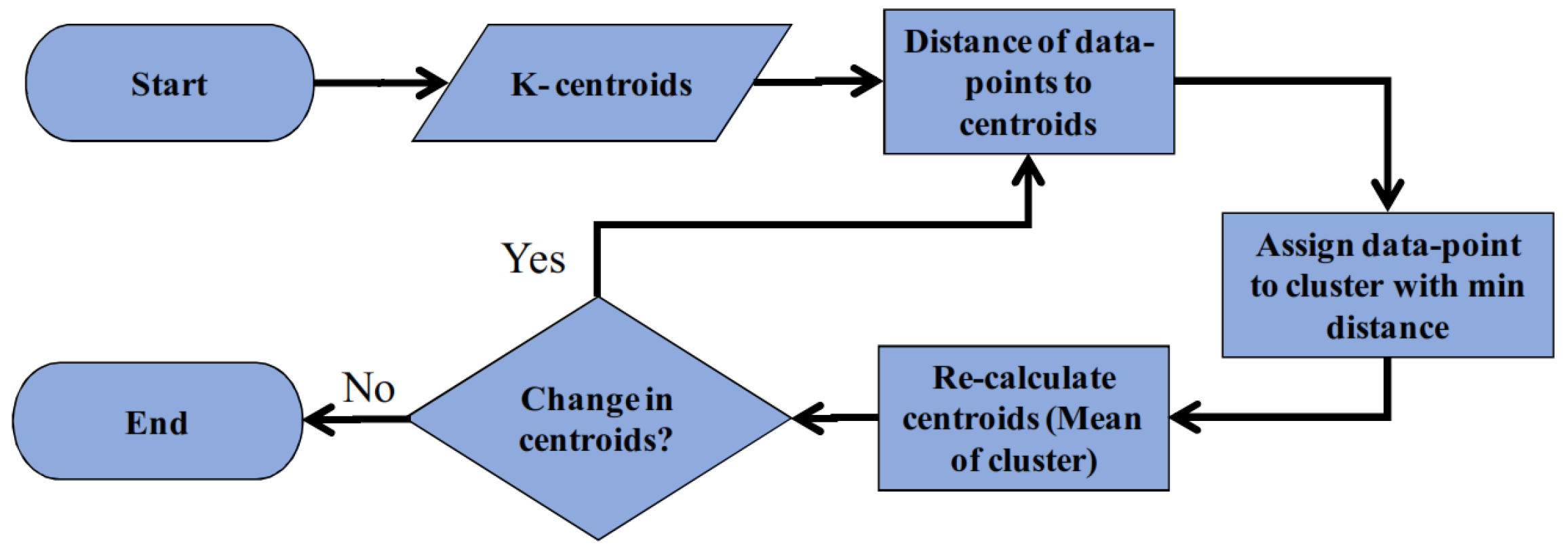
3.3. Image Segmentation Using K-Means Clustering

The region of interest (ROI) is defined as the subset of pixels within an image requiring further operations to be performed. To extract foreground information of olive trees as the ROI from the image, image segmentation technique is used. Various segmentation techniques can be used, out of which K-Means clustering is performed.

3.3.1. K-Means Clustering

K-Means clustering is a type of unsupervised learning that divides unlabeled data into non-overlapping groups [20]. The algorithm performs the iterative assignment of each data point to one of the K groups based on the least distance of centroids to their feature space. The process is repeated until centroids reach to their final constant positions. For the input of K number of clusters and respective centroids, data points representing olive trees are clustered and extracted. The flow diagram of the process is shown in Figure 2.

3.3.2. Centroid Selection

The centroid is a key data point around which clustering is performed. It is similar to any other data point represented with feature vector selected randomly or through a mechanism. In the proposed methodology, K numbers of centroids are selected under a mechanism [21] for better clustering, as it affects speed and performance, which is given mathematically as given in Equation (5),

$$C_i=i*\frac{m}{k+1}$$

(5)

where m is the maximum intensity value of the image determined from the histogram, k is the number of clusters and $C_i$ is the ith cluster centroid where i takes the value of 1, 2, 3, k.

3.4. Feature Extraction

The segments extracted as a result of clustering may include both olive trees and other ground components due to similar intensity levels. Features from those individual segments are extracted and a feature vector is formed. Olive trees when viewed from above show resemblance towards blob-like structures exhibiting distinct characteristics of size and color. The features extracted are grouped together forming a single feature vector. The statistical feature vector is calculated for each of the extracted foreground segment.

Table 1. Extracted statistical features from the images.

* Sr No.	Feature	Size of Feature Vector	Description
1	Mean of Red band	1×1	Average value of pixels in red band
2	Mean of Blue band	1×1	Average value of pixels in blue band
3	Mean of Green band	1×1	Average value of pixels in green band
4	Area	1×1	Number of pixels in a segment
5	Combined Features	1×4	Mean values of the color of the segment and its size

* Sr No: Serial Number.

lists the mentioned features along with the combined vector of those features.

3.5. Classification

Classification is one of most widely used technique in machine learning to predict the output belonging to a class label y based on input features x. Features extracted in the previous section are used to train and test multiple supervised learning algorithms. These include Naive Bayes, Support Vector Machine, Multi-layer Perceptron, and Random Forests.

3.5.1. Naive Bayes Classifier

Naive Bayes (NB) is a supervised learning technique based on the Bayes theorem [22]. It works on a naive assumption of independence among the features relating the conditional and marginal probabilities that two events occurred randomly. For an input x = (x1, x2, x3, xd), a d-dimensional feature vector with no output class label, the algorithm predicts the class based on the Bayes theorem. Let C be a class variable with class labels as $C_j$ with j = 1,2,3..k.$P\left(C_j\right)$ is the prior probability of class $C_j$. $P(x-C_j)$ is the likelihood of the object belonging to the class $C_j$ and $P\left(x\right)$ is the prior probability of the predictor. The posterior probability of a class $C_j$ given the predictor x as $P(C_j-x)$ as shown in Equation (6) as,

$$\begin{array}{c}\hfill P\left(C_j\right|x)=\frac{P\left(C_j\right)P\left(x\right|C_j)}{P\left(x\right)}\end{array}$$

(6)

In the above equation, the class $C_j$ is assigned to the input x based on the highest probability among all the classes. The independence of features among one another is given in Equation (7),

$$\begin{array}{c}\hfill P\left(x\right|C_j)=\prod _{j=1}^{k}P\left(x\right|C_j)\end{array}$$

(7)

The Naive Bayes classifier is based on the above equations and its naive assumption leads to simpler calculation and faster data processing. The two equations can be combined together summarizing the algorithm, as shown in Equation (8),

$$\begin{array}{c}\hfill j=arg\underset{j}{max}P\left(C_j\right)\prod _{i=1}^{d}P\left(x^i\right|C_j)\end{array}$$

(8)

where the $P\left(x\right)$ is omitted as it is the same for all the class.

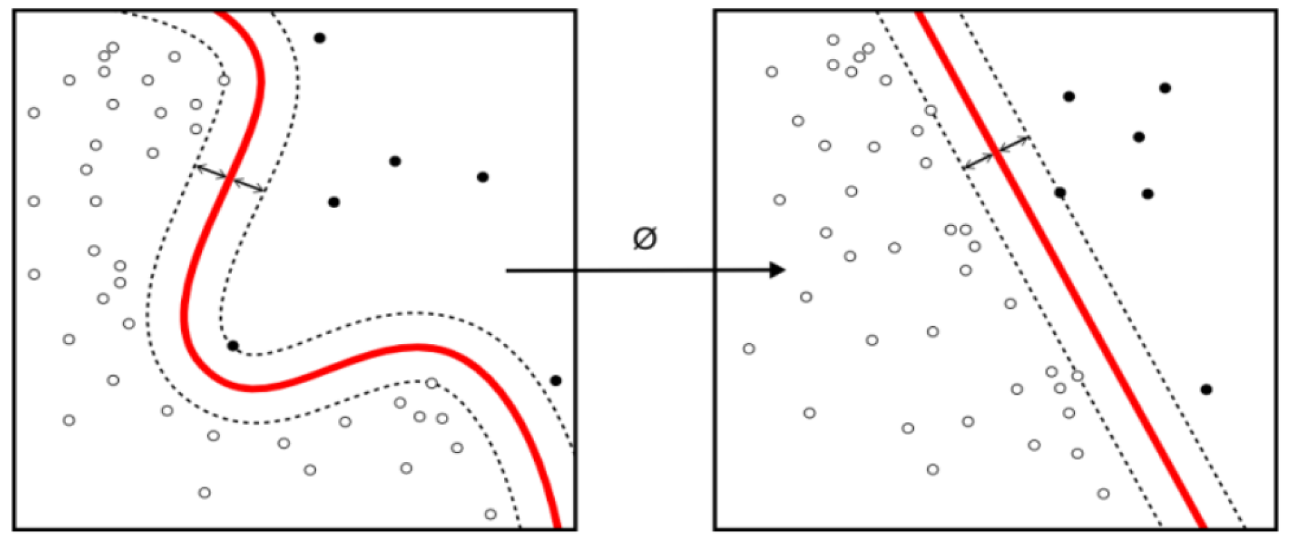
3.5.2. Support Vector Machines

Support Vector Machines (SVM) are a set of supervised learning methods proposed by Vapnik in 1995 that work by minimizing the classification error to maximize the geometric margin between the classes [23]. The classifier works by finding the right hyperplane to separate the data points into required classes. Once the hyperplane is determined, the testing samples are predicted to be on either side of the plane. Mathematically, the hyperplane is given by Equation (9),

$$w·x+b=0$$

(9)

where x is an N-dimensional input vector, w is a weight vector described as w = (w1, w2, w3...wn), and b represents the bias of the model and is a scalar quantity described as the perpendicular distance from hyper-plane to the origin.

3.5.3. Random Forest

Random Forest is a classification algorithm consisting of tree-structured classifiers (h(x,${\odot }_k$ and k = 1,2), where (${\odot }_k$) is given as an independent identical distribution of random vectors [24]. Each tree casts a vote for the input x. Random Forest is based on an ensemble technique grouping classifiers such as decision trees and classifies the instances by summation of their individual votes. It is very popular among the classification algorithms due to its high performance.

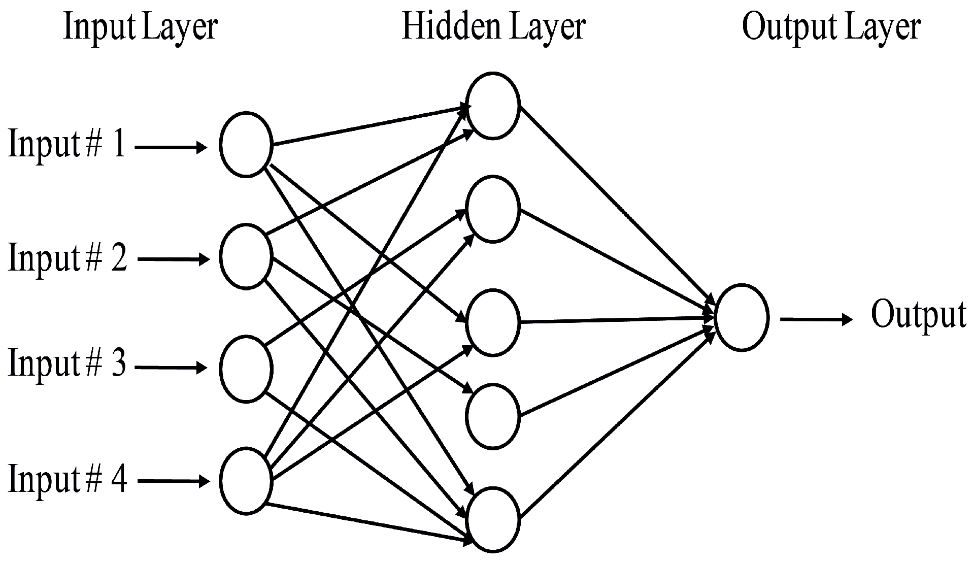
3.5.4. Multi-Layer Perceptron (MLP)

Artificial Neural networks (ANN) are non-parametric flexible models comprised of several layers of computing elements called as nodes. The input signal is received by each node through external inputs and is processed locally through the transfer function. Transfer function outputs the transformed signal to other nodes. In MLP, all nodes and layers are arranged in a feed-forward manner [25].

Any input vector fed into the network is propagated from the first layer as an input layer, passing through the hidden layers, towards the last layer as the output layer. Three-layer MLP is a commonly used ANN structure for binary classification problems such as of olive tree detection. An example of an MLP with one hidden layer and one output node is shown in Figure 3. The hyperplane is represented by a dashed line in Figure 4.

Statistical features extracted from the segments are fed into the classifiers resulting in a binary classification map, indicating the classified olive trees along with non-olive objects. Classification accuracy is calculated, and correctly classified olive trees are recorded giving the total olive tree count.

4. Materials and Methods

This section describes the dataset used to evaluate our proposed method. It also discusses the parameters on which the performance of our method was measured and gauged.

4.1. Dataset

To evaluate the performance of our proposed algorithm, images were acquired from the SIGPAC viewer of the Ministry of Environment and Rural and Marine Affairs (http://sigpac.mapa.es/fega/visor/). The interface spans the communities of Spanish territory captured in the form of satellite images. Among those communities is the Castilla La Mancha, covering the province of Toledo, which is significant for a high concentration of olive production [28].

Around 110 images in the visible spectrum with a spatial resolution of 1m and of uniform image sample size of 300×300 were taken from the satellite images. Parameters defining the center of the area by Universal Transverse Mercator (UTM) corresponded to Huso 30 with X = 411,943.23 and Y = 4,406,332.6 [3]. Images taken from the viewer included multiple land covers including houses, roads, shrubs and bushes, rocks, and olive trees. For each image, the land covers were marked, providing the ground truth information necessary in the classification stage.

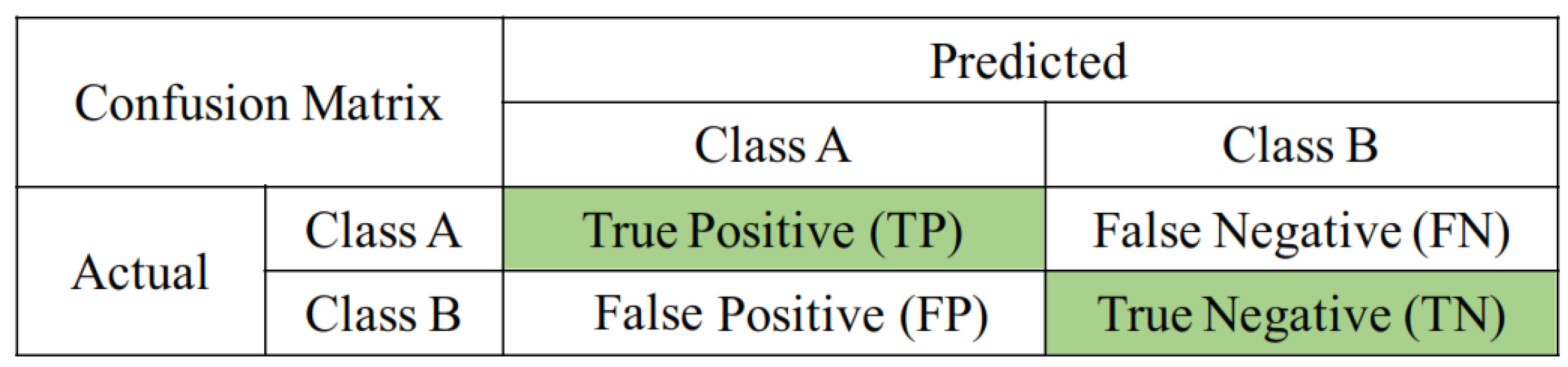
4.2. Performance Evaluation Metrics

Information about how well a classification system has performed in predicting the testing samples against their ground truth values was recorded in a confusion matrix or error matrix, as shown in Figure 5.

True Positive (TP) and True Negative (TN) are the correctly classified test samples of positive class and negative class, respectively. Positive class in our system represents the olive trees, whereas negative class represents the non-olive objects. False Positive (FP) and False Negative (FN) are the mis-classifications of test samples of positive and negative classes, respectively, into other classes. Using the information from the confusion matrix, various performance evaluation metrics were calculated, which are briefly discussed below.

4.2.1. Overall Accuracy (OA)

It is represented as the ratio of the number of correctly predicted items to a total number of items to predict. In our binary classification problem, it is calculated as the ratio of correctly predicted olive and non-olive tree samples to the total number of samples. Mathematically, it is given as Equation (10),

$$Overallaccuracy=\frac{TP+TN}{(TP+TN+FN+FP)}*100$$

(10)

4.2.2. Commission Error (CE)

Commission error, also known as False Positive rate, is defined as the mis-classification of an object being labeled as a true class actually belonging to the false one. The rate at which a non-olive sample is classified as an olive one is given as in Equation (11) as,

$$CommissionErrorRate=\frac{FP}{FP+TN}$$

(11)

4.2.3. Omission Error (OE)

Omission error, also known as False Negative rate, is defined as the mis-classification of an object being labeled to a false class belonging to the true one. It is the rate at which an olive tree sample is classified as a non-olive one. Omission error is given in Equation (12) as,

$$OmissionErrorRate=\frac{FN}{FN+TP}$$

(12)

4.2.4. Estimation Error (EE)

It is given as the error in estimation of the number of samples within a given region relative to the actual number of samples within that region. It is the representation of error between the estimated number of trees and the actual number of trees to be estimated. Mathematically, it is given in Equation (13) as,

$$\begin{array}{c}\hfill e_t=\left(\frac{N_{estimated}-N_{actual}}{N_{actual}}\right)\times 100\end{array}$$

(13)

4.2.5. Finding the Optimal Value of K

The value of K in K-Means clustering specifies the number of groups to be formed, which can be determined by clustering itself. Our methodology utilizes the elbow method [29] to find the optimal value of K, which works by measuring the intracluster distances between cluster points and their centroids given by Sum of Squared Error (SSE), as in Equation (14),

$$\begin{array}{c}\hfill SSE=\sum _{i=1}^k{\sum _{x\in C_i}dist(x,C_i)}^2\end{array}$$

(14)

where dist is the Euclidean distance between the cluster members x and cluster centroid $C_i$. Moving from smaller to larger value of K, the SSE decreases, giving less variation in the intracluster distance. The point with an abrupt decrease in the SSE gives the value of K. Our method uses the value of K as 4.

5. Experimental Results

Step-by-step results are described, elaborated, and compared with the existing techniques below. The proposed methods were tested on a desktop computer with $Core™$ i7 7700HQ and 2.80 GHz.

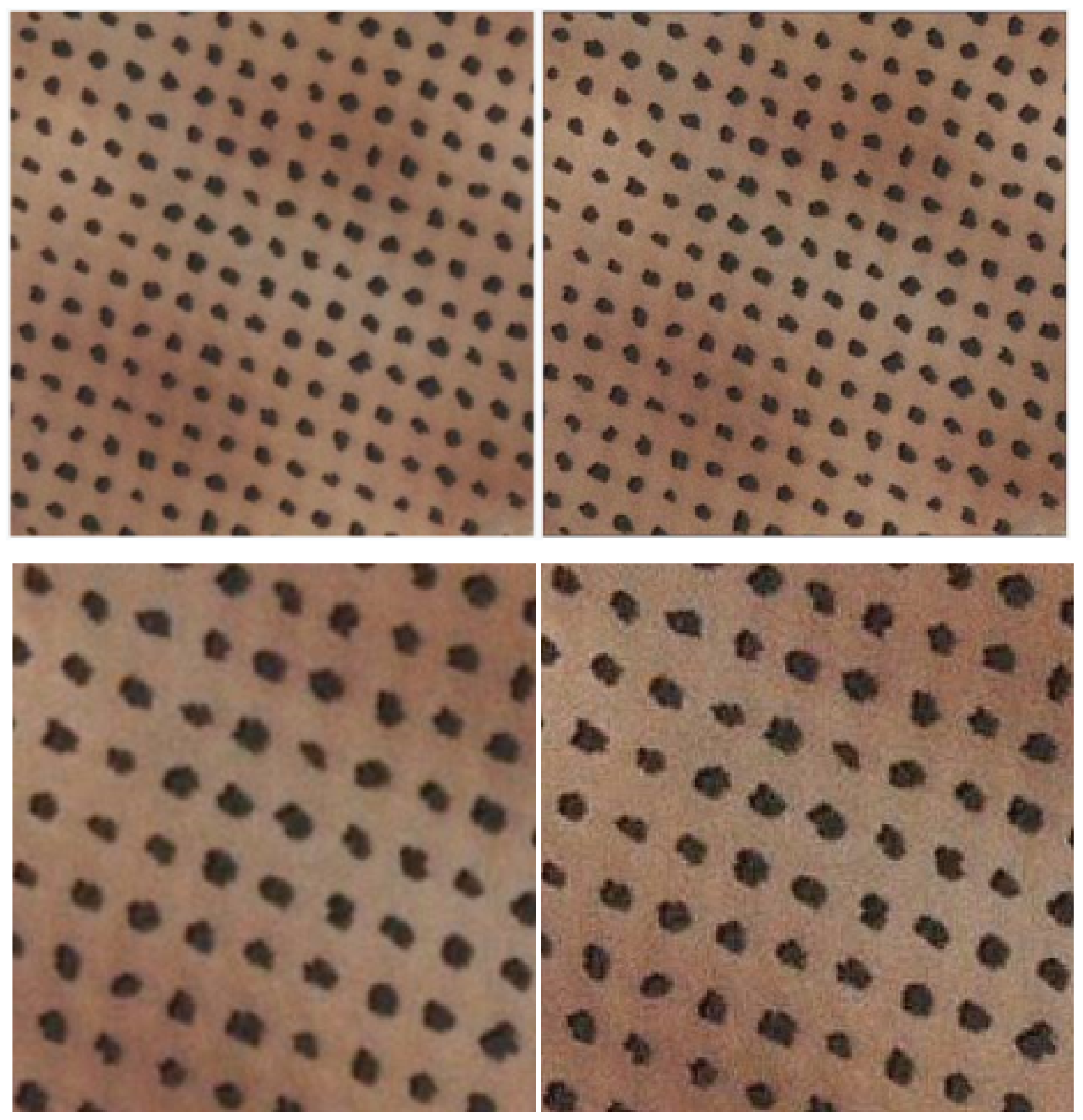
5.1. Image Pre-Processing Results

As mentioned in Section 3.2, LoG was utilized for the pre-processing of images where input colored images were pre-processed to reduce any noise or errors obscuring the required information. Images were smoothened, normalizing any noise in the image followed by the sharpening through Laplacian filter. Some examples of pre-processed images are shown in Figure 6.

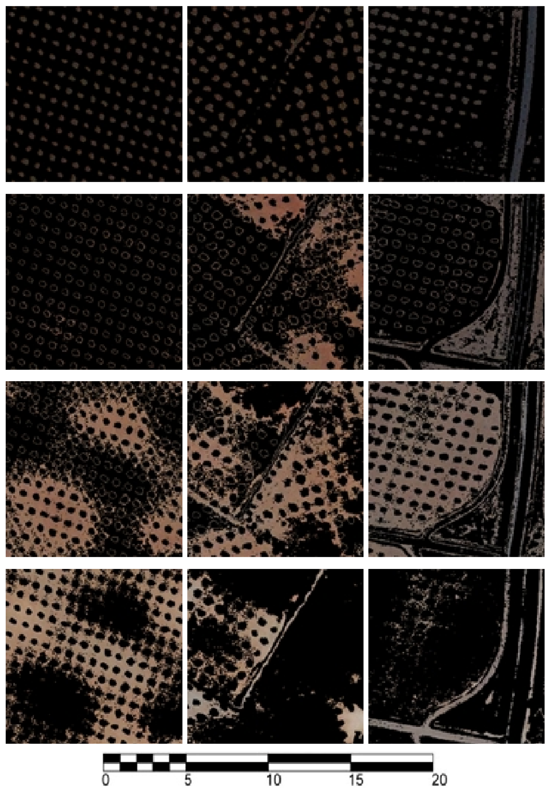
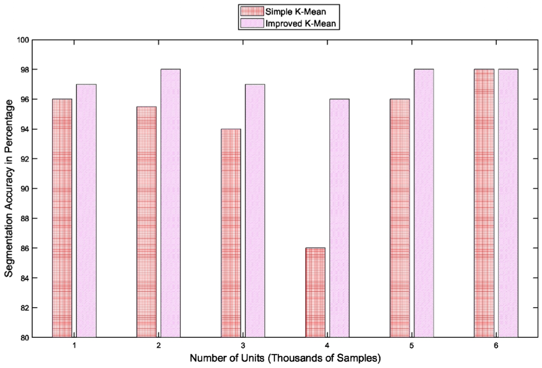
5.2. Image Segmentation Results

The ROI in the images are the olive trees and were extracted out of the background information using K-Mean clustering, as discussed in Section 3.3. The average optimal value for number of clusters was obtained as 4. The value of 4 was determined based on the abrupt change in SSE for varying values of K. The segments formed as result of K-Mean clustering with a value of K as 4 are shown in Figure 7.

Segmentation results were validated by measuring the segmentation accuracy of the proposed K-Means clustering method and results were recorded. The segmentation accuracy of the method was determined by calculating the overlapping percentage of resultant image with the marked ground truth information. It was calculated through Jaccard Analysis, measuring the ratio of intersection between segmentation result A and marked ground data B to the union of both A and B. Mathematically, it is given in Equation (15) as,

$$J(A,B)=\frac{|A\cup B|}{|A\cap B|}$$

(15)

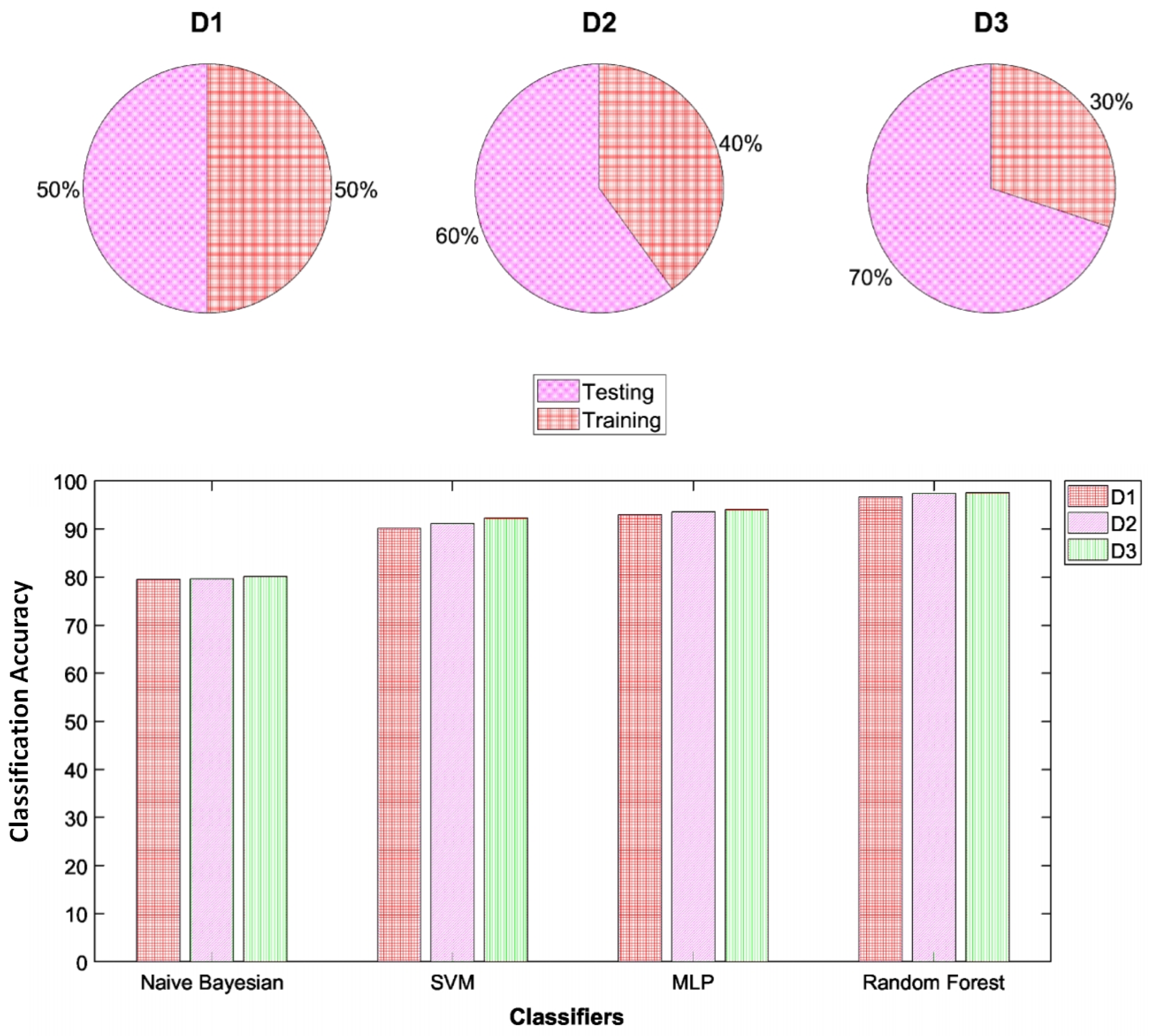
5.3. Classification Results

Statistical features extracted from the segments of images including both olive and non-olive tree components were fed into the classifiers SVM, Naive Bayesian, Random Forest, and MLP.

Data samples denoted by D1, D2, and D3 represent the training to testing ratios of 50 to 50, 60 to 40, and 70 to 30, respectively, as shown in Figure 8. It was observed that by increasing the training ratio from 50% to 70%, classifiers showed an increase in the classification results. Naive Bayesian, SVM, Multi-Layer Perceptron, and Random Forest showed an overall accuracy of 79.5%, 90.1%, 92.9%, and 96.6%, respectively, over the 50 to 50 division ratio.

Increasing the training samples to 60% of the total data samples, the overall accuracy for the classifiers increased to 79.6%, 91.1%, 93.5%, and 97.3%, respectively. The ratio of 70% for training samples resulted in the highest overall accuracy, with Naive Bayesian at 80.1%, SVM at 92.3%, MLP at 94%, and Random Forest performing best at 97.52%.

Confusion matrices for classifiers trained and tested at D3 proportion are shown in

Table 2. Confusion matrices of the Olive Tree classification by four classifiers for D3 Division (table constructed as shown in Figure 5).

* SVM	Tree	Non-Tree	Naive Bayesian	Tree	Non-Tree
Tree	2971	10	Tree	2653	328
Non-tree	360	1474	Non-tree	630	1204
** MLP	Tree	Non-Tree	Random Forest	Tree	Non-Tree
Tree	2891	90	Tree	2936	45
Non-tree	197	1637	Non-tree	74	1760

* SVM: Support Vector Machine. ** MLP: Multi-Layer Perceptron.

, whereas comparison of classifiers for D3 division (70% training and 30% testing) is shown in

Table 3. Performance evaluation of classifiers presented as percentage values.

Classification Algorithm	* OA	** CE	*** OE	**** EE
Random Forest	97.5	0.04	0.015	0.97
MLP	94.0	0.10	0.03	3.5
SVM	92.3	0.19	0.003	10.1
Naive Bayesian	80.1	0.34	0.11	11.7

* OA, Overall Accuracy; ** CE, Commission Error; *** OE, Omission Error; **** EE, Estimation Error.

.

6. Discussion

This section discusses the overall results achieved by the proposed method and draws a comparative analysis of computational time with the utilization of both versions of K-Means segmentation. It also draws a comparative analysis between the proposed method and existing techniques.

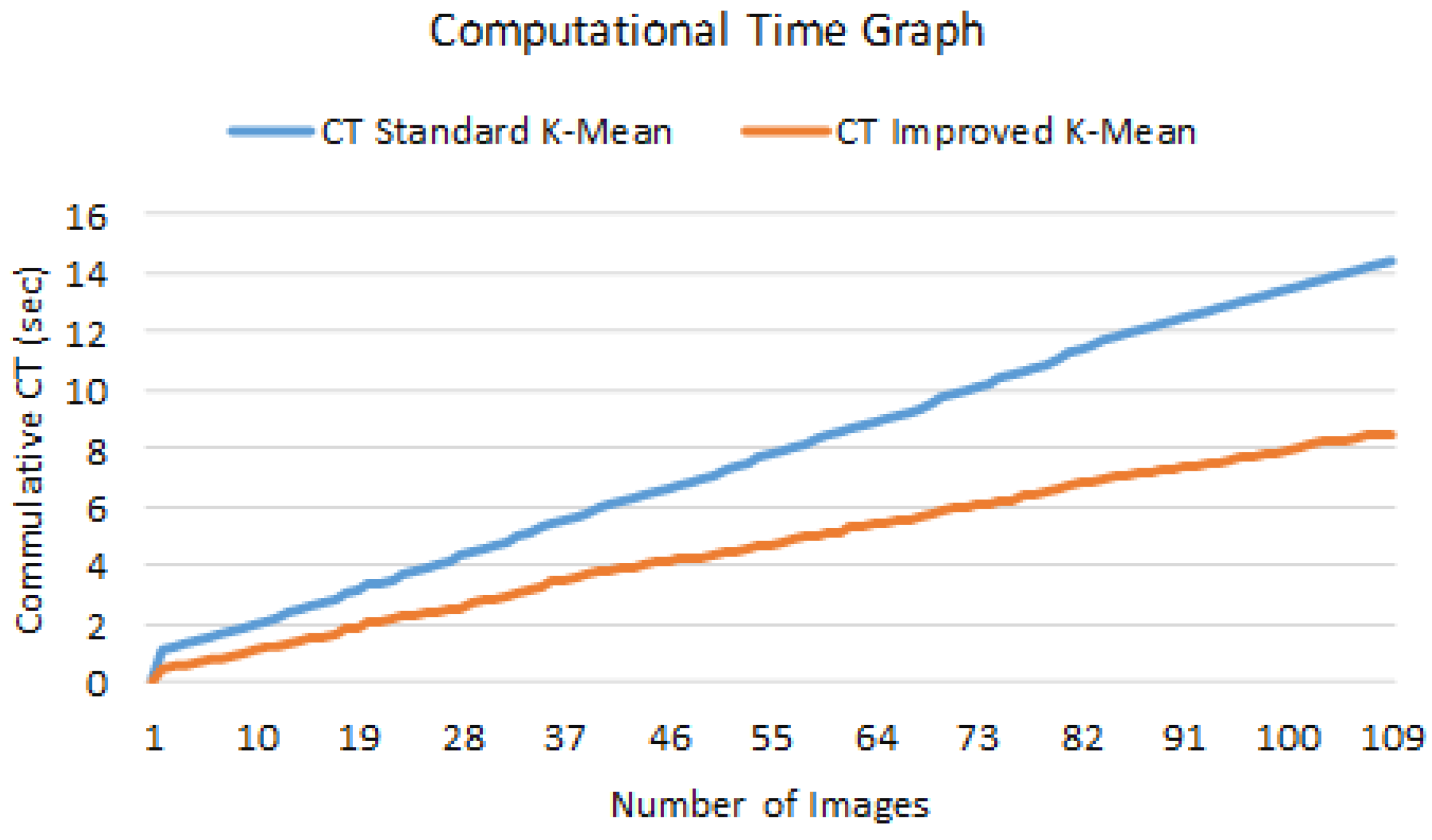
6.1. Comparative Analysis with Simple K-Mean

Standard K-Means technique initializes the centroids by random selection among the data points. The clustering is performed around the selected centers as they move towards the final position during the iterative process. The initial selection of centroids plays an important role in the overall performance of the clustering algorithm, affecting clustering speed along with the improvement in results. A comparative analysis between the two versions of K-Mean clustering is shown in Figure 9.

It can be seen for Unit 6 both K-Mean variations performed equally well. However, for images with low contrast between the background and foreground, centroid selected K-Means seemed to outperform the other, such as for Units 1–3 and 5. Centroid selected K-Means was able to detect young olive trees, outperforming the simple approach by a far margin for Unit 4.

Centroid selection speeds up the convergence of initial centroids to their final position, reducing the number of iterations by half that of standard K-Means. A reduced number of iterations results in reduced computational complexity.

The average computational time for an image using improved K-Mean comes out to be 78 ms, whereas the standard/simple K-Mean results in 131 ms of average computational time. A comparison of the computational time (CT) between the two variants of K-Mean is shown in Figure 10.

6.2. Comparative Analysis with Benchmark Schemes

Our proposed methodology and its results were compared with the existing techniques for olive detection and its enumeration. The comparison drew on the parameters of the dataset, the number of images used, the spectrum showing the processed information size, and the performance evaluation metrics. A tabular form of the analysis is given in

Table 4. Comparative analysis of the proposed scheme vs. benchmark schemes.

Technique	Dataset	No of Images	Spectrum	OA	CE	OE	EE
Proposed Methodology	SIGPAC Viewer	110	RGB	97.5	4 in 100	1 in 100	0.97
Reticular matching [9]	Quickbird	N/A	Grey-scale	98	5 in 100	7 in 100	1.24
Laplacian Maxima [7]	Quickbird / IKONOS	N/A	Grey-scale	N/A	N/A	N/A	N/A
GPC [11]	IKONOS-2	1	RGB	96	N/A	N/A	3.68
K-mean Clustering [5]	SIGPAC viewer	N/A	RGB	N/A	0 in 6	1 in 6	N/A
Fuzzy logic [10]	SIGPAC viewer	1	RGB	N/A	0 in 6	1 in 6	N/A
Red band Thresholding + NDVI [8]	Quickbird	N/A	4-bands	N/A	N/A	N/A	1.3
Counting Olive Trees in Heterogeneous Plantations [6]	Acquired Aerial Images	N/A	4-bands	N/A	N/A	N/A	13
Object-based olive grove mapping [12]	Multi-sensor imagery	4	4-bands	84.3	N/A	N/A	N/A
Multi-level thresholding [15]	SIGPAC viewer	95	Gray-scale	96	3 in 100	3 in 100	1.2

N/A: Not Available.

.

For the spectral information of the imagery utilized, Ionis et al.’s ACE method [6] combining the red band and NDVI-based thresholding followed by the blob detection showed an estimation error of 1.24%. Chemin et al.’s [4] thresholding-based method for the binarization of the multi-spectral image followed by the localization of centers to detect the possible olive trees showed an estimation error of almost 13%. Jan Peters et al. [10] work based on developing synergy models combining sensor data followed by four-step classification algorithm showed an overall accuracy of 84.3%. The above-mentioned techniques showed promising results, achieving high accuracies; however, all the techniques utilized multi-spectral information, leading to the added computational cost.

Some techniques utilize only the color band spectral information or less. J. Gonzales’ reticular matching technique identified olive trees within a particular area [7] using grayscale images. The probabilistic approach to detect olive trees combining the probability of a tree in a reticle along with its probability of being an olive tree showed promising results with an overall accuracy of 98%. In [9], Yakoub et al proposed classifying morphological features of ground objects from satellite imagery using GPC, detecting about 96% of the olive trees. Juan et al. proposed method of K-Means clustering [3] over SIGPAC viewer imagery, identifying almost all olive trees with a commission rate of zero and an omission rate of one in six of the test cases.

Juan et al. utilized the same imagery over the application of fuzzy logic [8] and showed quite similar results as per K-Means technique. The above-mentioned techniques showed accurate results with less processing information, however lacked diversity in terms of the number of images along with the ground classes. Karantzalos et al.’s [5] method of detection of olive trees consisted of pre-processing the input images acquired from QUICKBIRD satellite followed by detecting the local maxima of Laplacian as olive trees. Their study provided no such statistical data to measure the performance of the algorithm.

Our five-step classification model was tested over varying ratios of dataset distribution and resulted in high accuracy, ensuring the accuracy and robustness of our algorithm. Our proposed method addressed the shortcomings in existing techniques by accurately identifying olive trees, leading to a reliable tree count. This novel approach of five-step classification in olive tree detection validated over images having diverse ground data over color spectrum with an overall accuracy of 97.5% significantly contributes to the existing literature.

7. Conclusions

In this paper, we propose an automated method for the detection and enumeration of olive trees comprising of a multi-step classification-based implementation model. The model took an RGB image acquired from the SIGPAC Viewer as an input. The input image went through a stage of pre-processing that removed any additive noise followed by segmentation using the improved K-means clustering algorithm. Statistical features were extracted over the connected pixels in each of the segments and were classified using SVM, MLP, Random Forest, and Naive Bayesian. Among the classifiers, Random Forest outperformed the rest with an overall accuracy of 97.5% at 70 to 30 ratio of training to testing. Our technique with such accuracy, diversity, and enough samples for the proper training of the classifiers outperformed the previous techniques. It overcame the limitations of false tree count along with computationally expensive based accurate systems, devising a computationally efficient, accurate, and robust olive tree detection algorithm. As future work, we will incorporate more features to improve the feature extraction method as well as the classification. We look forward to the detection of olive trees using deep learning.

References

1. Radinovsky, L. 2017/18 Worldwide Olive Oil Production Estimates Compared. Available online: http://www.greekliquidgold.com/index.php/en/news/292-2017-18-worldwide-olive-oil-production-estimates-compared (accessed on 6 December 2019).
2. Srestasathiern, P.; Rakwatin, P. Oil palm tree detection with high resolution multi-spectral satellite imagery. Remote Sens. 2014, 6, 9749–9774. [Google Scholar] [CrossRef] [Green Version]
3. Moreno-Garcia, J.; Linares, L.J.; Rodriguez-Benitez, L.; Solana-Cipres, C. Olive trees detection in very high resolution images. In Information Processing and Management of Uncertainty in Knowledge-Based Systems. Applications. IPMU 2010; Communications in Computer and Information Science; Hüllermeier, E., Kruse, R., Hoffmann, F., Eds.; Springer: Berlin/Heidelberg, Germany, 2010; Volume 81, pp. 21–29. [Google Scholar]
4. Chemin, Y.H.; Beck, P.S. A Method to Count Olive Trees in Heterogenous Plantations from Aerial Photographs. Geoinformatics 2017. [Google Scholar] [CrossRef]
5. Karantzalos, K.; Argialas, D. Towards Automatic Olive Tree Extraction from Satellite Imagery. 2014. Available online: https://pdfs.semanticscholar.org/4ba8/1e085c2bde7b925b36906697b1a49794290b.pdf (accessed on 7 December 2019).
6. Daliakopoulos, I.N.; Grillakis, E.G.; Koutroulis, A.G.; Tsanis, I.K. Tree crown detection on multispectral vhr satellite imagery. Photogramm. Eng. Remote Sens. 2009, 75, 1201–1211. [Google Scholar] [CrossRef] [Green Version]
7. González, J.; Galindo, C.; Arevalo, V.; Ambrosio, G. Applying Image Analysis and Probabilistic Techniques for Counting Olive Trees in High-Resolution Satellite Images. In Advanced Concepts for Intelligent Vision Systems. ACIVS 2007; Lecture Notes in Computer Science; Blanc-Talon, J., Philips, W., Popescu, D., Scheunders, P., Eds.; Springer: Berlin/Heidelberg, Germany, 2007; Volume 4678, pp. 920–931. [Google Scholar]
8. Moreno-Garcia, J.; Jimenez, L.; Rodriguez-Benitez, L.; Solana-Cipres, C.J. Fuzzy logic applied to detect olive trees in high resolution images. In Proceedings of the IEEE International Conference on Fuzzy Systems, Barcelona, Spain, 18–23 July 2010. [Google Scholar] [CrossRef]
9. Bazi, Y.; Al-Sharari, H.; Melgani, F. An automatic method for counting olive trees in very high spatial remote sensing images. In Proceedings of the 2009 IEEE International Geoscience and Remote Sensing Symposium, Cape Town, South Africa, 12–17 July 2009; pp. II-125–II-128. [Google Scholar] [CrossRef]
10. Peters, J.; van Coillie, F.; Westra, T.; de Wulf, R. Synergy of very high resolution optical and radar data for object-based olive grove mapping. Int. J. Geogr. Inf. Sci. 2011, 25, 971–989. [Google Scholar] [CrossRef]
11. Commission, E. Joint Research Centre. Available online: https://ec.europa.eu/info/departments/joint-\research-centre-en (accessed on 12 December 2019).
12. Bagli, S. Olicount v2. Technical Documentation, Joint Reseach Centre IPSC/G03/P/SKA/ska D (5217). 2005. Available online: https://www.scribd.com/document/324886236/Olicount-v2 (accessed on 14 December 2019).
13. Soubeyrand, S.; de Jerphanion, P.; Martin, O.; Saussac, M.; Manceau, C.; Hendrikx, P.; Lannou, C. Inferring pathogen dynamics from temporal count data: The emergence of xylella fastidiosa in france is probably not recent. New Phytol. 2018. [Google Scholar] [CrossRef] [Green Version]
14. Niblack, W. An Introduction to Digital Image Processing; Strandberg Publishing Company: Birkeroed, Denmark, 1985. [Google Scholar]
15. Khan, A.; Khan, U.; Waleed, M.; Khan, A.; Kamal, T.; Marwat, S.N.K.; Maqsood, M.; Aadil, F. Remote sensing: An automated methodology for olive tree detection and counting in satellite images. IEEE Access 2018, 6, 77816–77828. [Google Scholar] [CrossRef]
16. Bhosale, N.P.; Manza, R.R. A Review on Noise Removal Techniques From Remote Sensing Images. In Proceedings of the Radhai National Conference [CMS], Aurangabad, India, 25–26 April 2013. [Google Scholar] [CrossRef]
17. Noh, Z.M.; Ramli, A.R.; Hanafi, M.; Saripan, M.I.; Ramlee, R.A. Palm vein pattern visual interpretation using laplacian and frangi-based filter. Indones. J. Electr. Eng. Comput. Sci. 2018, 10, 578–586. [Google Scholar] [CrossRef]
18. Piao, W.; Yuan, Y.; Lin, H. A digital image denoising algorithm based on gaussian filtering and bilateral filtering. In Proceedings of the 4th Annual International Conference on Wireless Communication and Sensor Network (WCSN 2017), 2018; Available online: https://www.itm-conferences.org/articles/itmconf/pdf/2018/02/itmconf_wcsn2018_01006.pdf (accessed on 15 December 2019). [CrossRef] [Green Version]
19. Kong, H.; Akakin, H.C.; Sarma, S.E. A generalized laplacian of gaussian filter for blob detection and its applications. IEEE Trans. Cybern. 2013, 43, 1719–1733. [Google Scholar] [CrossRef] [PubMed]
20. Kalra, M.; Lal, N.; Qamar, S. K-Mean Clustering Algorithm Approach for Data Mining of Heterogeneous Data; Springer: Berlin, Germany, 2018; pp. 61–70. [Google Scholar]
21. Hussain, R.G.; Ghazanfar, M.A.; Azam, M.A.; Naeem, U.; Rehman, S.U. A performance comparison of machine learning classification approaches for robust activity of daily living recognition. Artif. Intell. Rev. 2018, 1–23. [Google Scholar] [CrossRef]
22. Chen, X.; Zeng, G.; Zhang, Q.; Chen, L.; Wang, Z. Classification of Medical Consultation Text Using Mobile Agent System Based on Naïve Bayes Classifier. In 5G for Future Wireless Networks. 5GWN 2017; Lecture Notes of the Institute for Computer Sciences, Social Informatics and Telecommunications Engineering; Long, K., Leung, V., Zhang, H., Feng, Z., Li, Y., Zhang, Z., Eds.; Springer: Cham, Switzerland, 2017; Volume 211. [Google Scholar] [CrossRef]
23. Cortes, C.; Vapnik, V. Support-Vector Networks. Mach. Learn. 1995, 20, 273–297. [Google Scholar] [CrossRef]
24. Mahesh, P. Random Forest classifier for remote sensing classification. Int. J. Remote Sens. 2005, 26, 217–222. [Google Scholar] [CrossRef]
25. Narang, A.; Batra, B.; Ahuja, A.; Yadav, J.; Pachauri, N. Classification of eeg signals for epileptic seizures using levenberg-marquardt algorithm based Multi-Layer Perceptron neural network. J. Intell. Fuzzy Syst. 2018, 34, 1669–1677. [Google Scholar] [CrossRef]
26. Mohamed, H.; Zahran, M.; Saavedra, O. Assessment of Artificial Neural Network for Bathymetry Estimation using High Resolution Satellite Imagery in Shallow Lakes: Case Study el Burullus Lake. In Proceedings of the Eighteenth International Water Technology Conference, IWTC18, Sharm ElSheikh, Egypt, 12–14 March 2015. [Google Scholar]
27. Duan, K.B.; Keerthi, S.S. Which Is the Best Multiclass SVM Method? An Empirical Study; Lect Notes in Computer Science; Springer: Berlin/Heidelberg, Germany, 2005; Volume 3541. [Google Scholar]
28. Camarsa, G.; Gardner, S.; Jones, W.; Eldridge, J.; Hudson, T.; Thorpe, E.; O’Hara, E. Life among the Olives: Good Practice in Improving Environmental Performance in the Olive Oil Sector; Official Publications of the European Union: Luxembourg, 2010; Available online: https://op.europa.eu/en/publication-detail/-/publication/53cd8cd1-272f-4cb8-b7b5-5c100c267f8f (accessed on 15 December 2019).
29. Sai Krishna, T.V.; Yesu Babu, A.; Kiran Kumar, R. Determination of Optimal Clusters for a Non-hierarchical Clustering Paradigm K-Means Algorithm. In Proceedings of International Conference on Computational Intelligence and Data Engineering; Lecture Notes on Data Engineering and Communications Technologies; Chaki, N., Cortesi, A., Devarakonda, N., Eds.; Springer: Singapore, 2018; Volume 9. [Google Scholar] [CrossRef]
Figure 1. Workflow of algorithm for automatic detection of olive trees.
Remotesensing 12 00760 g001
Figure 2. Flow diagram of K-Mean algorithm.
Remotesensing 12 00760 g002
Figure 3. A hypothetical example of the Multi-Layer Perceptron (MLP) network used for classification [26].
Remotesensing 12 00760 g003
Figure 4. The ability of the SVM to classify datasets that are not linearly separable [27].
Remotesensing 12 00760 g004
Figure 5. Confusion Matrix.
Remotesensing 12 00760 g005
Figure 6. Image pre-processing results. The first column represents the input image and its zoomed in version, whereas the second column refers to the corresponding results after pre-processing.
Remotesensing 12 00760 g006
Figure 7. Image Segmentation Results for K set as 4. The first row represents the first cluster; the second row is the second cluster; and the third and fourth rows correspond to the third and fourth clusters, respectively. The scale bar represents the scaling ratio of 1 cm to 400 m.
Remotesensing 12 00760 g007
Figure 8. Comparative analysis of Naive Bayesian, Support Vector Machine (SVM), Multi-Layer Perceptron (MLP), and Random Forest over division ratios D1 (50% testing, 50% training), D2 (40% testing, 60% training), and D3 (30% testing, 70% training).
Remotesensing 12 00760 g008
Figure 9. Comparison of segmentation accuracy between the Simple K-Means and Improved K-Means.
Remotesensing 12 00760 g009
Figure 10. Comparison of Computational Time (CT) between the Simple K-Means and Improved K-Means.
Remotesensing 12 00760 g010