Estimation of Hourly Sea Surface Salinity in the East China Sea Using Geostationary Ocean Color Imager Measurements


Abstract
1. Introduction
2. Materials and Methods
2.1. Materials
2.1.1. GOCI Rrs Data
2.1.2. I-ORS Data
2.1.3. Group for High Resolution Sea Surface Temperature (GHRSST) SST Data
2.1.4. SMAP Data
2.2. Methods
2.2.1. GOCI Data Preprocessing
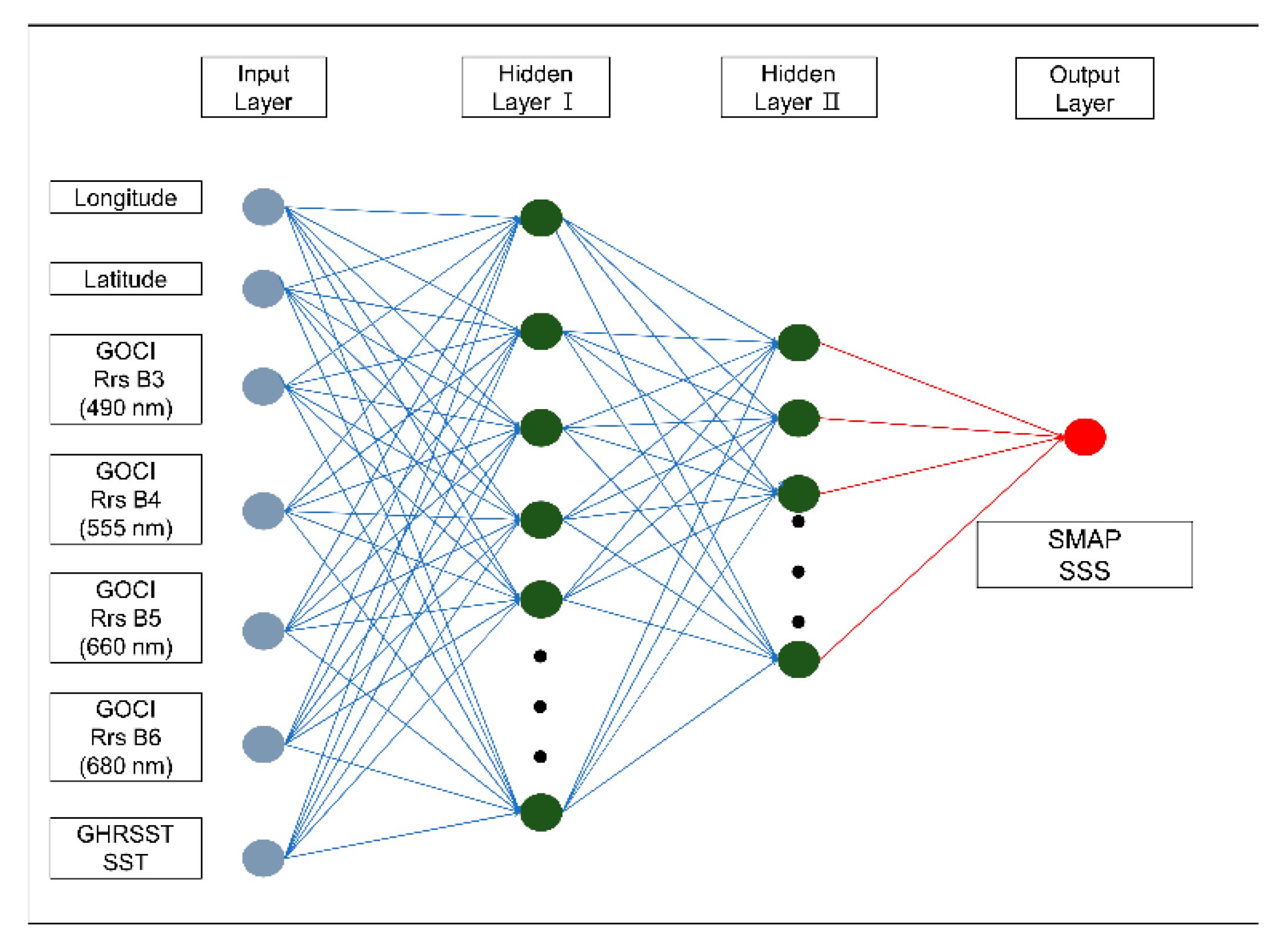
2.2.2. MPNN
3. Results
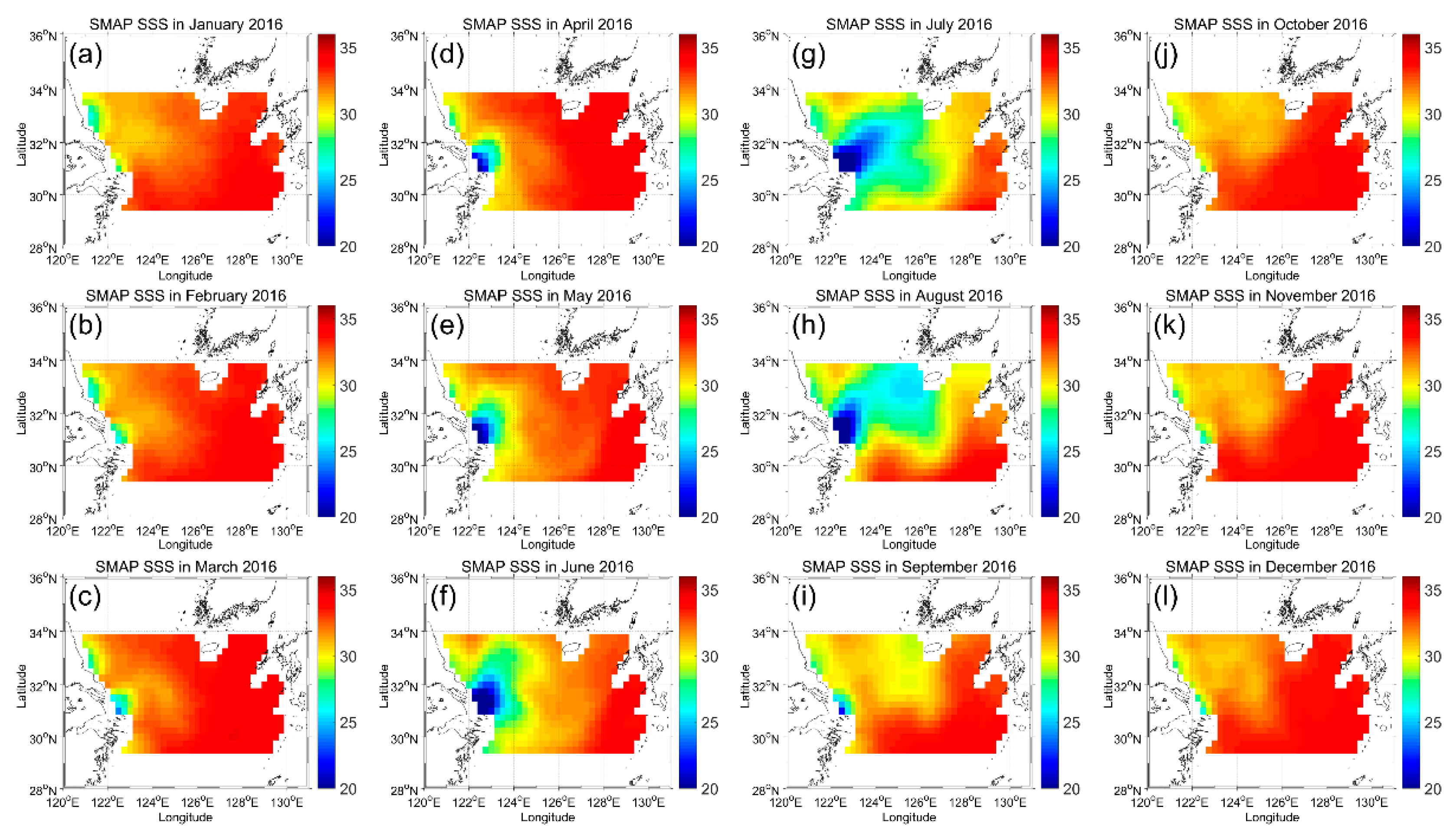
3.1. Model Performance Compared to SMAP SSS
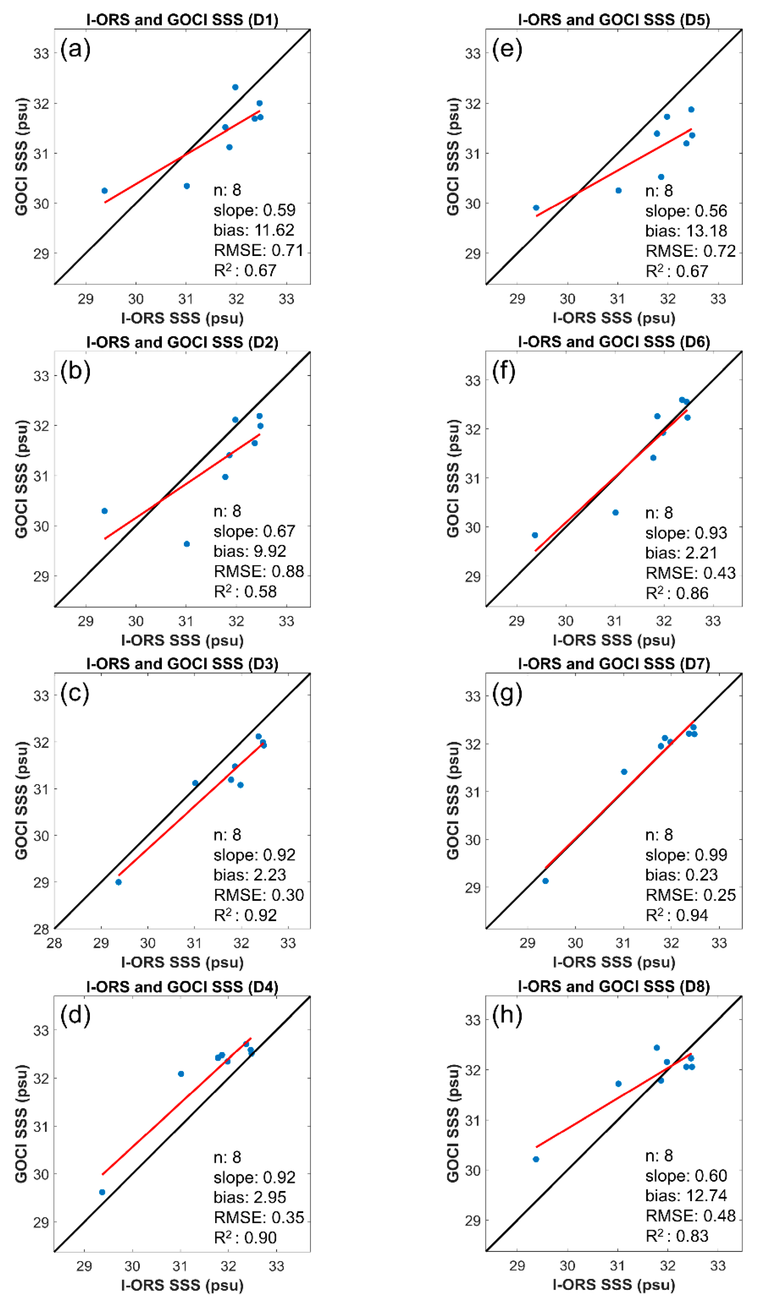
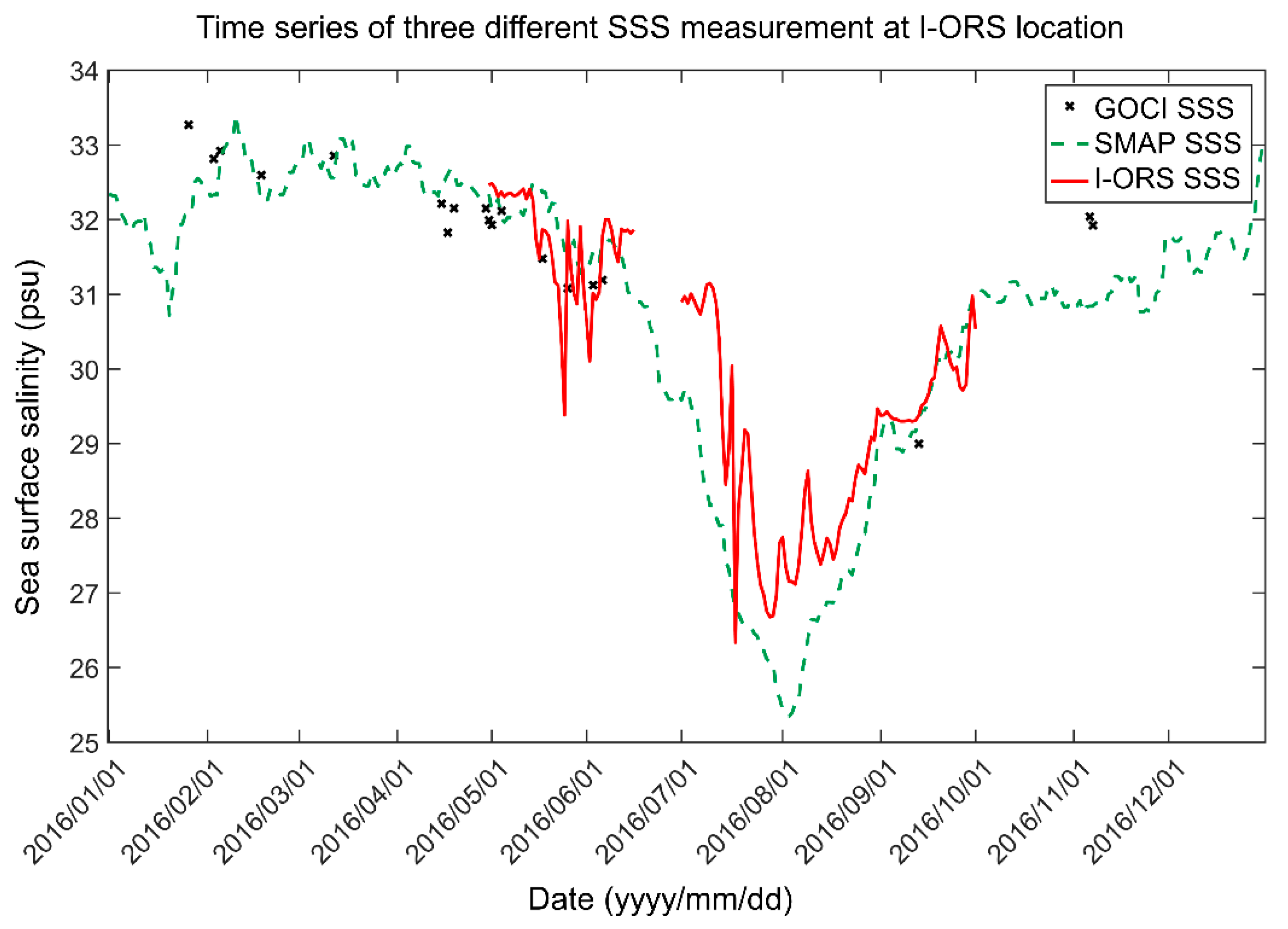
3.2. Model Performance Compared to I-ORS SSS
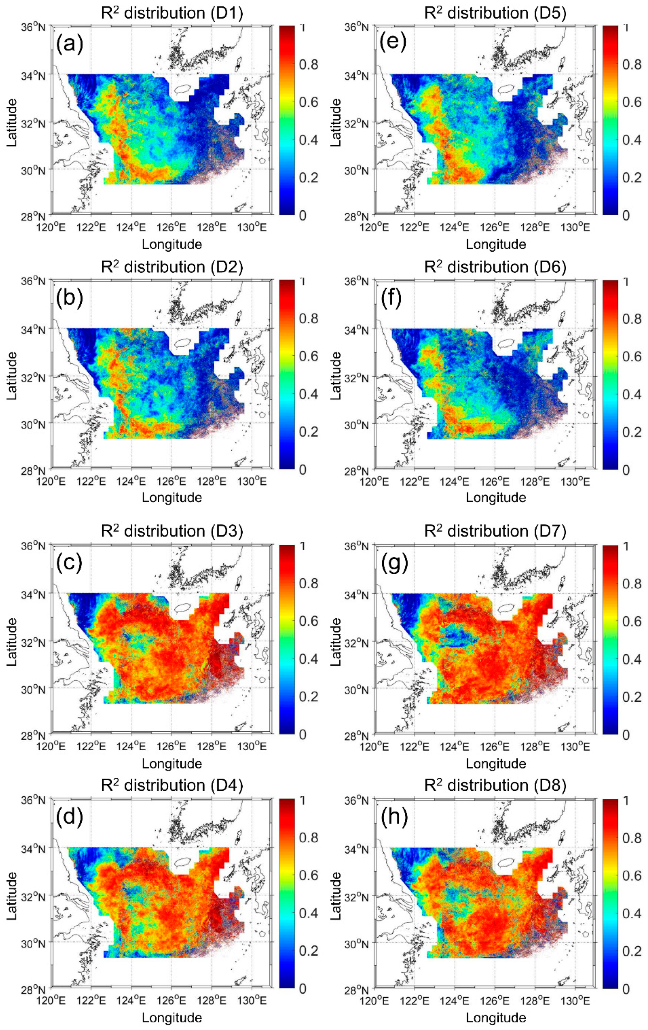
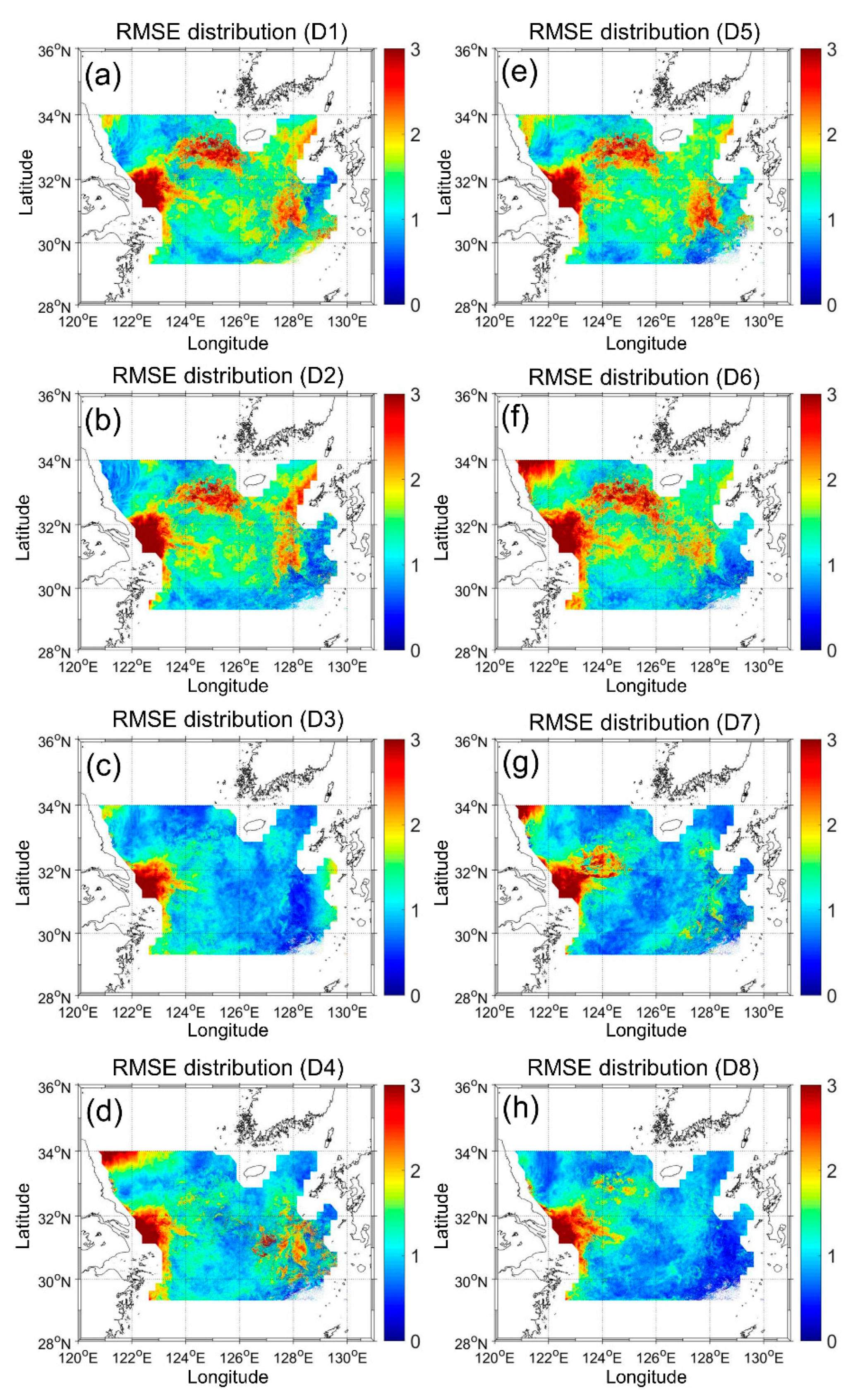
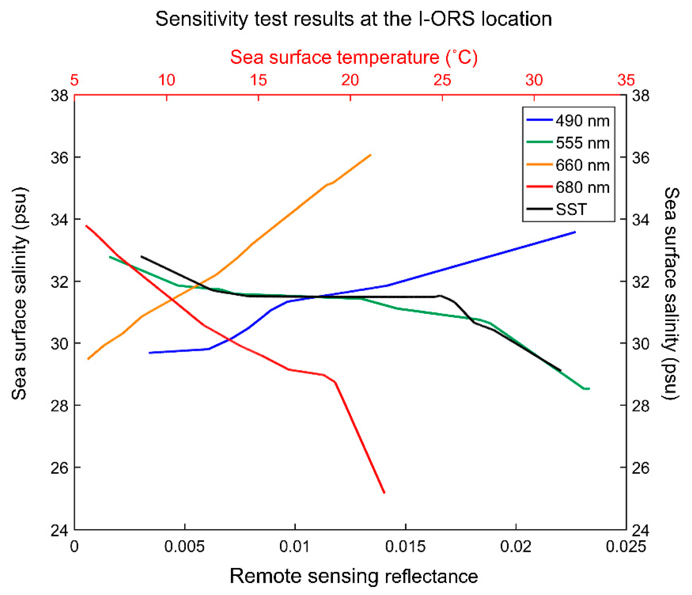
3.3. Importance of Input Parameters
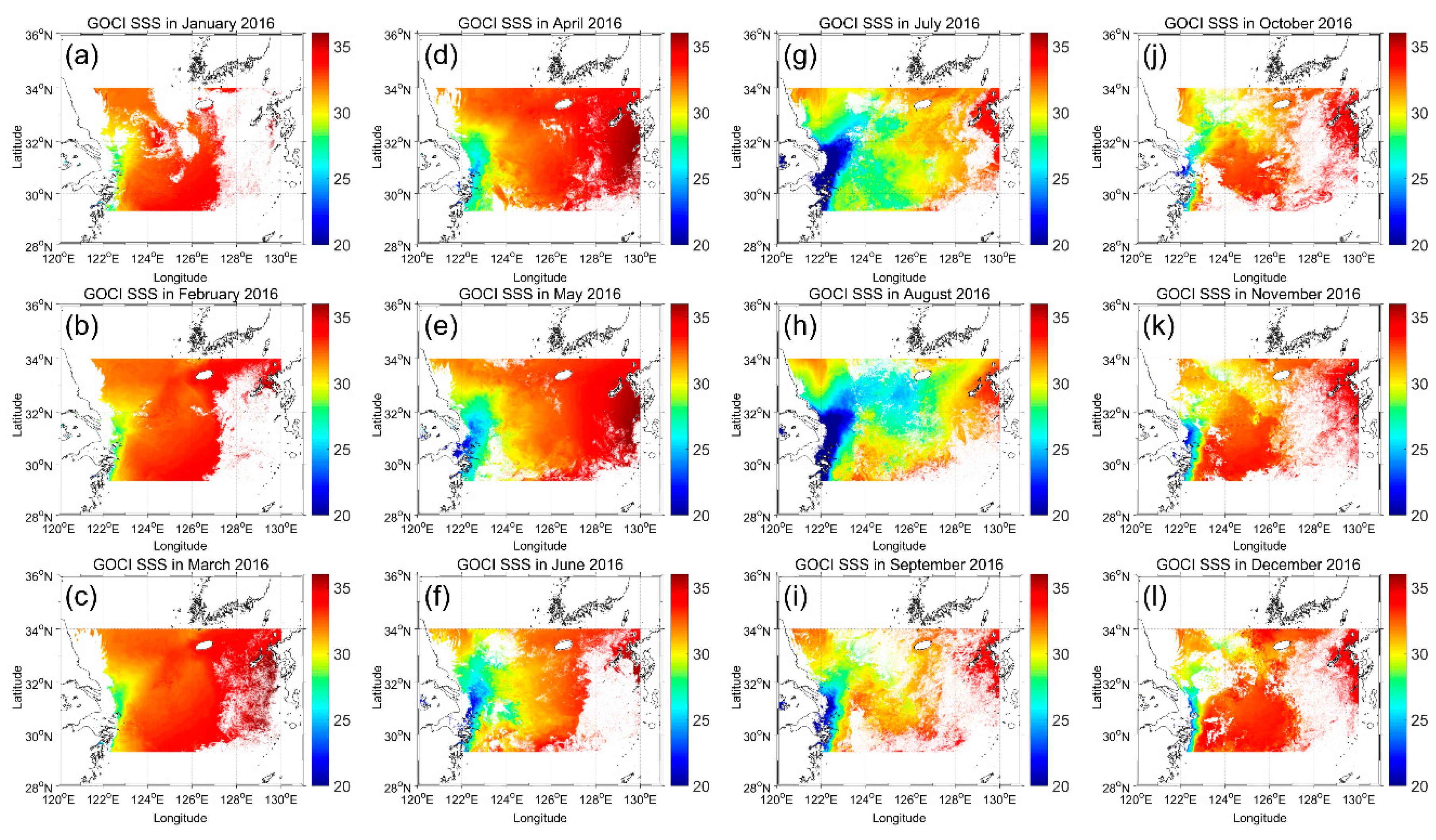
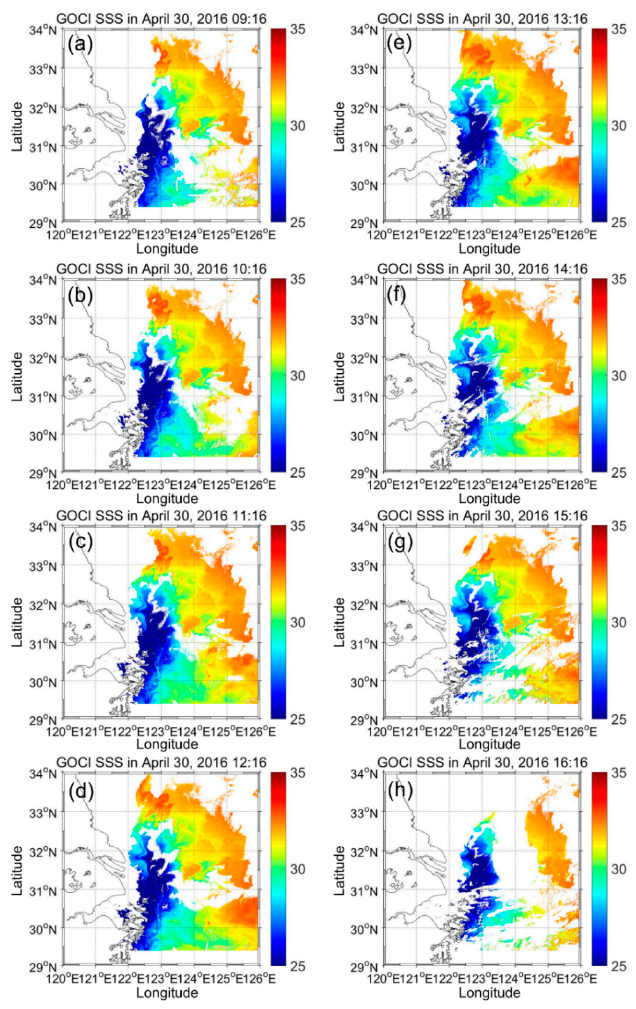
3.4. Validation of the GOCI SSS
4. Discussion
5. Conclusions
Author Contributions
Funding
Conflicts of Interest
References
- Chen, C.; Zhu, J.; Beardsley, R.C.; Franks, P.J. Physical-biological sources for dense algal blooms near the Changjiang River. Geophys. Res. Lett. 2003, 30, 1515–1518. [Google Scholar] [CrossRef]
- Lee, N.K.; Suh, Y.S.; Kim, Y.S. Satellite remote sensing to monitor seasonal horizontal distribution of resuspended sediments in the East China Sea. J. Korean Assoc. Geogr. Inf. Stud. 2003, 6, 151–161. [Google Scholar]
- Moon, J.H.; Pang, I.C.; Yoon, J.H. Response of the Changjiang diluted water around Jeju Island to external forcings: A modeling study of 2002 and 2006. Cont. Shelf Res. 2009, 29, 1549–1564. [Google Scholar] [CrossRef]
- Kim, H.C.; Yamaguchi, H.; Yoo, S.; Zhu, J.; Okamura, K.; Kiyomoto, Y.; Tanaka, K.; Kim, S.W.; Park, T.; Ishizaka, J. Distribution of Changjiang diluted water detected by satellite chlorophyll-a and its interannual variation during 1998–2007. J. Oceanogr. 2009, 65, 129–135. [Google Scholar] [CrossRef]
- Moon, J.H.; Hirose, N.; Yoon, J.H.; Pang, I.C. Offshore detachment process of the low-salinity water around Changjiang Bank in the East China Sea. J. Phys. Oceanogr. 2010, 40, 1035–1053. [Google Scholar] [CrossRef]
- Bai, Y.; Pan, D.; Cai, W.J.; He, X.; Wang, D.; Tao, B.; Zhu, Q. Remote sensing of salinity from satellite-derived CDOM in the Changjiang River dominated East China Sea. J. Geophys. Res. Ocean. 2013, 118, 227–243. [Google Scholar] [CrossRef]
- Kim, S.B.; Lee, J.H.; Matthaeis, P.; Yueh, S.; Hong, C.S.; Lee, J.H.; Lagerloef, G. Sea surface salinity variability in the E ast C hina S ea observed by the A quarius instrument. J. Geophys. Res. Ocean. 2014, 119, 7016–7028. [Google Scholar] [CrossRef]
- Lee, D.K.; Kwon, J.I.; Son, S. Horizontal distribution of Changjiang Diluted Water in summer inferred from total suspended sediment in the Yellow Sea and East China Sea. Acta Oceanol. Sin. 2015, 34, 44–50. [Google Scholar] [CrossRef]
- Moon, J.-H.; Kim, T.; Son, Y.B.; Hong, J.-S.; Lee, J.-H.; Chang, P.-H.; Kim, S.-K. Contribution of low-salinity water to sea surface warming in the summer of 2016. Prog. Oceanogr. 2019, 175, 68–88. [Google Scholar]
- Suh, Y.S.; Jang, L.H.; Lee, N.K. Detection of low salinity water in the northern East China Sea during summer using ocean color remote sensing. Korean J. Remote Sens. 2004, 20, 153–162. (in Korean). [Google Scholar]
- Yoon, H.J.; Cho, H.K. A study on the diluted water from the Yangtze River in the East China Sea using satellite data. J. Korean Assoc. Geogr. Inf. Stud. 2005, 8, 33–43. (in Korean). [Google Scholar]
- Zhou, F.; Xuan, J.L.; Ni, X.B.; Huang, D.J. A preliminary study of variations of the Changjiang Diluted Water between August of 1999 and 2006. Acta Oceanol. Sin. 2009, 28, 1–11. [Google Scholar]
- KHOA. High sea temperature phenomenon of August 2016. In Unusual ocean analysis report; KHOA (Korea Hydrographic and Oceanographic Agency): Busan, Republic of Korea, 2016; Volume 1. (in Korean) [Google Scholar]
- Koblinsky, C.J.; Hildebrand, P.; LeVine, D.; Pellerano, F.; Chao, Y.; Wilson, W.; Yueh, S.; Lagerloef, G. Sea surface salinity from space: Science goals and measurement approach. Radio Sci. 2003, 38. [Google Scholar] [CrossRef]
- Entekhabi, D.; Njoku, E.G.; O’Neill, P.E.; Kellogg, K.H.; Crow, W.T.; Edelstein, W.N.; Kimball, J. The soil moisture active passive (SMAP) mission. Proc. IEEE 2010, 98, 704–716. [Google Scholar] [CrossRef]
- Font, J.; Camps, A.; Borges, A.; Martín-Neira, M.; Boutin, J.; Reul, N.; Kerr, Y.H.; Hahne, A.; Mecklenburg, S. SMOS: The challenging sea surface salinity measurement from space. Proc. IEEE 2009, 98, 649–665. [Google Scholar] [CrossRef]
- Kerr, Y.H.; Waldteufel, P.; Wigneron, J.P.; Delwart, S.; Cabot, F.; Boutin, J.; Escorihuela, M.J.; Font, J.; Reul, N.; Juglea, S.E.; et al. The SMOS mission: New tool for monitoring key elements of the global water cycle. Proc. IEEE 2010, 98, 666–687. [Google Scholar] [CrossRef]
- Geiger, E.F.; Grossi, M.D.; Trembanis, A.C.; Kohut, J.T.; Oliver, M.J. Satellite-derived coastal ocean and estuarine salinity in the Mid-Atlantic. Cont. Shelf Res. 2013, 63, S235–S242. [Google Scholar] [CrossRef]
- Chen, S.; Hu, C. Estimating sea surface salinity in the northern Gulf of Mexico from satellite ocean color measurements. Remote Sens. Environ. 2017, 201, 115–132. [Google Scholar] [CrossRef]
- Mohammed, P.N.; Aksoy, M.; Piepmeier, J.R.; Johnson, J.T.; Bringer, A. SMAP L-band microwave radiometer: RFI mitigation prelaunch analysis and first year on-orbit observations. IEEE Trans. Geosci. Remote. Sens. 2016, 54, 6035–6047. [Google Scholar] [CrossRef]
- Nakada, S.; Kobayashi, S.; Hayashi, M.; Ishizaka, J.; Akiyama, S.; Fuchi, M.; Nakajima, M. High-resolution surface salinity maps in coastal oceans based on geostationary ocean color images: quantitative analysis of river plume dynamics. J. Oceanogr. 2018, 74, 287–304. [Google Scholar] [CrossRef]
- Chen, R.F. In situ fluorescence measurements in coastal waters. Org. Geochem. 1999, 30, 397–409. [Google Scholar] [CrossRef]
- Binding, C.E.; Bowers, D.G. Measuring the salinity of the Clyde Sea from remotely sensed ocean colour. Estuar. Coast. Shelf Sci. 2003, 57, 605–611. [Google Scholar] [CrossRef]
- Del Vecchio, R.; Blough, N.V. Spatial and seasonal distribution of chromophoric dissolved organic matter and dissolved organic carbon in the Middle Atlantic Bight. Mar. Chem. 2004, 89, 169–187. [Google Scholar] [CrossRef]
- Sasaki, H.; Siswanto, E.; Nishiuchi, K.; Tanaka, K.; Hasegawa, T.; Ishizaka, J. Mapping the low salinity Changjiang Diluted Water using satellite-retrieved colored dissolved organic matter (CDOM) in the East China Sea during high river flow season. Geophys. Res. Lett. 2008, 35. [Google Scholar] [CrossRef]
- Ahn, Y.H.; Shanmugam, P.; Moon, J.E.; Ryu, J.H. Satellite remote sensing of a low-salinity water plume in the East China Sea. Ann. Geophys. Atmos. Hydrospheres Space Sci. 2008, 26, 2019–2035. [Google Scholar] [CrossRef]
- Liu, R.; Zhang, J.; Yao, H.; Cui, T.; Wang, N.; Zhang, Y.; An, J. Hourly changes in sea surface salinity in coastal waters recorded by Geostationary Ocean Color Imager. Estuarine Coast. Shelf Sci. 2017, 196, 227–236. [Google Scholar] [CrossRef]
- Sun, D.; Su, X.; Qiu, Z.; Wang, S.; Mao, Z.; He, Y. Remote Sensing Estimation of Sea Surface Salinity from GOCI Measurements in the Southern Yellow Sea. Remote Sens. 2019, 11, 775. [Google Scholar] [CrossRef]
- Hu, C.; Muller-Karger, F.E.; Biggs, D.C.; Carder, K.L.; Nababan, B.; Nadeau, D.; Vanderbloemen, J. Comparison of ship and satellite bio-optical measurements on the continental margin of the NE Gulf of Mexico. Int. J. Remote Sens. 2003, 24, 2597–2612. [Google Scholar] [CrossRef]
- Choi, J.K.; Park, Y.J.; Ahn, J.H.; Lim, H.S.; Eom, J.; Ryu, J.H. GOCI, the world’s first geostationary ocean color observation satellite, for the monitoring of temporal variability in coastal water turbidity. J. Geophys. Res. Ocean. 2012, 117. [Google Scholar] [CrossRef]
- Doxaran, D.; Lamquin, N.; Park, Y.J.; Mazeran, C.; Ryu, J.H.; Wang, M.; Poteau, A. Retrieval of the seawater reflectance for suspended solids monitoring in the East China Sea using MODIS, MERIS and GOCI satellite data. Remote Sens. Environ. 2014, 146, 36–48. [Google Scholar] [CrossRef]
- Son, Y.B.; Gardner, W.D.; Richardson, M.J.; Ishizaka, J.; Ryu, J.H.; Kim, S.H.; Lee, S.H. Tracing offshore low-salinity plumes in the Northeastern Gulf of Mexico during the summer season by use of multispectral remote-sensing data. J. Oceanogr. 2012, 68, 743–760. [Google Scholar] [CrossRef]
- O’Reilly, J.E.; Maritorena, S.; Mitchell, B.G.; Siegel, D.A.; Carder, K.L.; Garver, S.A.; Kahru, M.; McClain, C. Ocean color chlorophyll algorithms for SeaWiFS. J. Geophys. Res. Ocean. 1998, 103, 24937–24953. [Google Scholar] [CrossRef]
- Ryu, J.H.; Han, H.J.; Cho, S.; Park, Y.J.; Ahn, Y.H. Overview of geostationary ocean color imager (GOCI) and GOCI data processing system (GDPS). Ocean Sci. J. 2012, 47, 223–233. [Google Scholar] [CrossRef]
- Lie, H.J.; Cho, C.H.; Lee, J.H.; Lee, S. Structure and eastward extension of the Changjiang River plume in the East China Sea. J. Geophys. Res. Ocean. 2003, 108. [Google Scholar] [CrossRef]
- Ha, K.J.; Nam, S.; Jeong, J.Y.; Moon, I.J.; Lee, M.; Yun, J.; Jang, C.J.; Kim, Y.S.; Byun, D.S.; Shim, J.S.; et al. Observations utilizing Korean Ocean Research Stations and their Applications for Process Studies. Bull. Am. Meteorol. Soc. 2019, 100, 2061–2075. [Google Scholar] [CrossRef]
- Wu, Q.; Wang, X.; He, X.; Liang, W. Validation and Application of SMAP SSS Observation in Chinese Coastal Seas. In Coastal Environment, Disaster, and Infrastructure-A Case Study of China’s Coastline; Liang, X.S., Zhang, Y., Eds.; IntechOpen: London, UK, 2018; pp. 273–284. [Google Scholar]
- Lee, M.S.; Park, K.A.; Moon, J.E.; Kim, W.; Park, Y.J. Spatial and temporal characteristics and removal methodology of suspended particulate matter speckles from Geostationary Ocean Color Imager data. Int. J. Remote Sens. 2019, 40, 3808–3834. [Google Scholar] [CrossRef]
- Wei, J.; Lee, Z.; Shang, S. A system to measure the data quality of spectral remote-sensing reflectance of aquatic environments. J. Geophys. Res. Ocean. 2016, 121, 8189–8207. [Google Scholar] [CrossRef]
- Kingma, D.P.; Ba, J. Adam: A method for stochastic optimization. arXiv 2014, arXiv:1412.6980. [Google Scholar]
- Moh, T.; Cho, J.H.; Jung, S.K.; Kim, S.H.; Son, Y.B. Monitoring of the Changjiang River Plume in the East China Sea using a Wave Glider. J. Coast. Res. 2018, 85 (sp1), 26–30. [Google Scholar] [CrossRef]
- Beardsley, R.C.; Limeburner, R.; Yu, H.; Cannon, G.A. Discharge of the Changjiang (Yangtze river) into the East China sea. Cont. Shelf Res. 1985, 4, 57–76. [Google Scholar] [CrossRef]
- Gitelson, A.A.; Schalles, J.F.; Hladik, C.M. Remote chlorophyll-a retrieval in turbid, productive estuaries: Chesapeake Bay case study. Remote Sens. Environ. 2007, 109, 464–472. [Google Scholar] [CrossRef]
- Shi, W.; Wang, M. Satellite observations of flood-driven Mississippi River plume in the spring of 2008. Geophys. Res. Lett. 2009, 36. [Google Scholar] [CrossRef]
- Shen, F.; Verhoef, W.; Zhou, Y.; Salama, M.S.; Liu, X. Satellite estimates of wide-range suspended sediment concentrations in Changjiang (Yangtze) estuary using MERIS data. Estuaries Coasts 2010, 33, 1420–1429. [Google Scholar] [CrossRef]
- Zhang, M.; Tang, J.; Dong, Q.; Song, Q.; Ding, J. Retrieval of total suspended matter concentration in the Yellow and East China Seas from MODIS imagery. Remote Sens. Environ. 2010, 114, 392–403. [Google Scholar] [CrossRef]
- Son, S.; Wang, M.; Shon, J.K. Satellite observations of optical and biological properties in the Korean dump site of the Yellow Sea. Remote Sens. Environ. 2011, 115, 562–572. [Google Scholar] [CrossRef]
- Son, S.; Wang, M. Water properties in Chesapeake Bay from MODIS-Aqua measurements. Remote Sens. Environ. 2012, 123, 163–174. [Google Scholar] [CrossRef]
- Shi, W.; Wang, M. Ocean reflectance spectra at the red, near-infrared, and shortwave infrared from highly turbid waters: A study in the Bohai Sea, Yellow Sea, and East China Sea. Limnol. Oceanogr. 2014, 59, 427–444. [Google Scholar] [CrossRef]
- Bricaud, A.; Claustre, H.; Ras, J.; Oubelkheir, K. Natural variability of phytoplanktonic absorption in oceanic waters: Influence of the size structure of algal populations. J. Geophys. Res. Ocean. 2004, 109. [Google Scholar] [CrossRef]


| Input dataset | Train R2 | Train RMSE (psu) | Validation R2 | Validation RMSE (psu) |
|---|---|---|---|---|
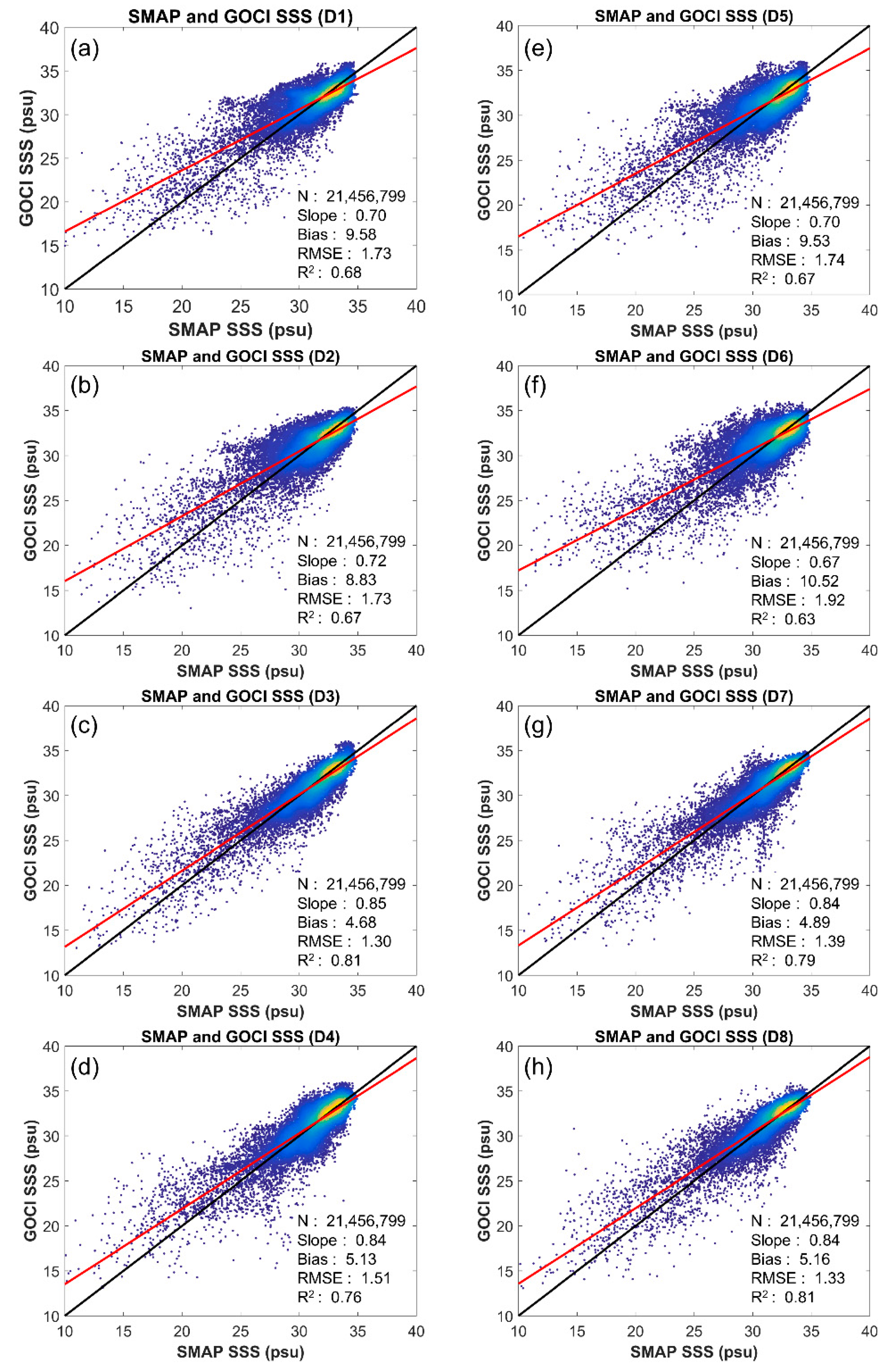
| Bands 3 to 6 (D1) | 0.75 | 1.73 | 0.68 | 1.73 |
| Bands 3 to 6 and R3 (D2) | 0.87 | 1.10 | 0.67 | 1.73 |
| Bands 3 to 6 and SST (D3) | 0.85 | 1.15 | 0.81 | 1.30 |
| Bands 3 to 6, R3, and SST (D4) | 0.87 | 1.10 | 0.76 | 1.51 |
| Bands 1 to 6 (D5) | 0.81 | 1.44 | 0.67 | 1.74 |
| Bands 1 to 6, R1, R2, and R3 (D6) | 0.79 | 1.50 | 0.63 | 1.92 |
| Bands 1 to 6 and SST (D7) | 0.85 | 1.28 | 0.79 | 1.39 |
| Bands 1 to 6, R1, R2, R3, and SST (D8) | 0.85 | 1.15 | 0.81 | 1.33 |
© 2020 by the authors. Licensee MDPI, Basel, Switzerland. This article is an open access article distributed under the terms and conditions of the Creative Commons Attribution (CC BY) license (http://creativecommons.org/licenses/by/4.0/).
Share and Cite
Kim, D.-W.; Park, Y.-J.; Jeong, J.-Y.; Jo, Y.-H. Estimation of Hourly Sea Surface Salinity in the East China Sea Using Geostationary Ocean Color Imager Measurements. Remote Sens. 2020, 12, 755. https://doi.org/10.3390/rs12050755
Kim D-W, Park Y-J, Jeong J-Y, Jo Y-H. Estimation of Hourly Sea Surface Salinity in the East China Sea Using Geostationary Ocean Color Imager Measurements. Remote Sensing. 2020; 12(5):755. https://doi.org/10.3390/rs12050755
Chicago/Turabian StyleKim, Dae-Won, Young-Je Park, Jin-Yong Jeong, and Young-Heon Jo. 2020. "Estimation of Hourly Sea Surface Salinity in the East China Sea Using Geostationary Ocean Color Imager Measurements" Remote Sensing 12, no. 5: 755. https://doi.org/10.3390/rs12050755
APA StyleKim, D.-W., Park, Y.-J., Jeong, J.-Y., & Jo, Y.-H. (2020). Estimation of Hourly Sea Surface Salinity in the East China Sea Using Geostationary Ocean Color Imager Measurements. Remote Sensing, 12(5), 755. https://doi.org/10.3390/rs12050755