Multi-Sensor Observations of Submesoscale Eddies in Coastal Regions

Abstract

The temporal and spatial variation in submesoscale eddies in the coastal region of Lianyungang (China) is studied over a period of nearly two years with high-resolution (0.03°, about 3 km) observations of surface currents derived from high-frequency coastal radars (HFRs). The centers and boundaries of submesoscale eddies are identified based on a vector geometry (VG) method. A color index (CI) representing MODIS ocean color patterns with a resolution of 500 m is used to compute CI gradient parameters, from which submesoscale features are extracted using a modified eddy-extraction approach. The results show that surface currents derived from HFRs and the CI-derived gradient parameters have the ability to capture submesoscale processes (SPs). The typical radius of an eddy in this region is 2–4 km. Although no significant difference in eddy properties is observed between the HFR-derived current fields and CI-derived gradient parameters, the CI-derived gradient parameters show more detailed eddy structures due to a higher resolution. In general, the HFR-derived current fields capture the eddy form, evolution and dissipation. Meanwhile, the CI-derived gradient parameters show more SPs and fill a gap left by the HFR-derived currents. This study shows that the HFR and CI products have the ability to detect SPs in the ocean and contribute to SP analyses.

1. Introduction

Submesoscale processes (SPs) are frequently observed as eddies, filaments and fronts, where the approximate scale ranges are 0.1–10 km in the horizontal, 0.01–1 km in the vertical, and between hours and days in time over open oceans [1]. The most fundamental characteristic difference between submesoscale and mesoscale is that the Rossby ($Ro)$ and Richardson numbers ($Ri$) are both close to $\mathcal{O}\left(1\right)$ for SPs. SPs have large vertical velocities which are typically several times larger than those associated with mesoscale processes; thus, they play a critical role in vertical transport [2,3], enhance bio-physical interactions, and provide a possible link between mixing and dissipation. Submesoscale buoyancy flux in SPs enhances seasonal restratification and the mixing of the mixed layer [4]. Submesoscale restratification can weaken submesoscale turbulence and enhance surface inertia-gravity waves [5]. The generation mechanisms of SPs may be summarized as: strain-induced frontogenesis, baroclinic instabilities in the mixed layer, turbulent thermal winds and topographic wakes [1,6,7]. Idealized numerical models under relevant theoretical frameworks may efficiently be employed in studies of SPs, which require high-resolution data of less than one hour in time and $\mathcal{O}\left(1\right)$ km in space [8,9].

Compared with numerical model simulations, the in situ observations at these scales are limited greatly by their ability to resolve the detailed horizontal and vertical structures of SPs [10,11,12,13,14,15,16]. However, in recent years, high-precision observations have mainly focused on some special submesoscale events and phenomena, due to increased sampling rates in time and space [6,11]. Remote-sensing observations can also be used to investigate SPs, such as surface currents derived by high-frequency radar [2,17,18,19], geostationary ocean color imagery (GOCI)-derived chlorophyll surface concentration maps, and colored dissolved organic matter [20], which are available at hourly and kilometer-scale resolutions. HFRs can provide information on ocean surface currents over a large, horizontal distance with high spatial-temporal resolution, which can reach up to 200 m in space (e.g., SeaSonde [21]) and 20 min in time. Meanwhile, satellite images can rarely observe SPs continuously because of their limitation in sampling frequency, contamination from high-frequency motions and incoherent internal tides. L. Pomale-Velázquez et al. [22] analyzed the characterization of mesoscale eddies and submesoscale eddies using satellite images (i.e., satellite-measured sea surface height anomalies, satellite-derived geostrophic velocity components, satellite chlorophyll-a (Chl-a) and available floating algae index images). HFRs were used to measure surface velocities off the coast of southwestern Puerto Rico, and it was found that they are capable of identifying submesoscale eddies lasting for 3 days. However, satellite products cannot capture these eddies for long time periods. Moreover, because certain satellite images, for example high-resolution radar images, show variable anomalies instantaneously, they can be used to obtain some characteristics of submesoscale eddies instantaneously. Although HFRs have previously been applied to study coastal submesoscale currents in other coastal regions, this is the first application of HFRs in characterizing submesoscale eddies in the Lianyungang area (Figure 1a); thus, we are able to improve our understanding of issues related to oceanography, relevant to port planning and fisheries management in Haizhou Bay.

In this area, there is one flow existing in the coastal regions: the Yellow Sea Coastal Current coming from the northwest [23]. The tidal current is characterized by regular semidiurnal currents (the M2 tide is the main constituent). The tidal current shows a rectilinear motion, where the direction of the flood (ebb) tide tends to be southwestward (northeastward) and winter tide currents are generally stronger than summer tide currents. In winter (summer), the major axis of the M2 tidal ellipse is $30.85\mathrm{cm}/\mathrm{s}$ ($28.53\mathrm{cm}/\mathrm{s}$) which shows that the local current is affected by the tidal currents [24]. The dominant bathymetric feature is the shallow coastal area, with a maximum water depth of 33 m. There is a shallow bank in the center of the region and a channel located between the bank and the 10 m isobath. The interaction between the tidal current and the bathymetry is the main driver for the generation of submesoscale eddies and filaments. Vortex stretching on the ebb and flood tides is considered to be closely linked to eddy generation and the local wind-driven currents also affect the distribution and movement of submesoscale eddies [2,25].

In order to detect submesoscale eddies, methods based on their geometric properties are applied. Traditionally, methods for automatic eddy detection have been mostly based on physical or geometric properties of the flow field [26,27]. Methods based on physical properties mostly identify eddies by comparing specified physical parameters, including pressure, the magnitude of sea level anomalies, vorticity, and various quantities derived from the velocity gradient tensor [26,28,29,30]. Methods based on the geometric properties include the winding-angle method [27,31,32], the vector geometry (VG) method [33], vector pattern matching [34] and the Clifford convolution [35]. Compared with methods based on physical properties, methods based on the geometric properties can better detect eddies and tend to consider a non-vortical structure as an eddy [36].

Dong et al. [37] used satellite-measured SST images to obtain the characteristics of ocean mesoscale eddies, which extracted most mesoscale signals limited by the coarse resolution of Remote Sensing System SST production. Here, Moderate Resolution Imaging Spectroradiometer (MODIS) ocean color patterns of resolution up to 500 m are applied to extract submesoscale signals, based on a similar approach proposed by Dong et al. [37]. A color index (CI, units: non-dimensional) represents the MODIS ocean color patterns, which are derived from an empirical approach proposed by Hu [38]. The empirical approach has been proven to validly remove sun glint and clouds and increase the data coverage. The CI has a significant correlation with the MODIS band-ratio Chl-a (<1 mg m⁻³) and is a good index to represent coastal color changes. Liu et al. [39] pointed out that mesoscale anticyclonic eddies in the Gulf of Mexico Loop Current system were accompanied by low CI values which indicated clear waters. Local CI increases (decreases) when submesoscale cyclonic (anticyclonic) eddies occur, while local SST decreases (increases) when submesoscale cyclonic (anticyclonic) eddies occur. This could help us understand the process by which eddies drive the upwelling of colder, nutrient rich waters that boost plankton production, the aggregation and retention of particles, etc. Because SST and CI have opposite responses to cyclonic and anticyclonic eddies, CI-derived gradient parameters are calculated by a modified method based on an automated approach to extract submesoscale signals. Zhang et al. [40] used two thresholds to determine the candidate boundaries for eddy detection. These two thresholds were determined after trial-and-error ananlyses of 625 sets of threshold values, which may not be applicable for other regions. Our modified method focuses on the gradient information only, without the need to use thermal wind approximation, such as in Dong et al. [37]. This is because the thermal wind approximation is not applicable for submesoscale eddies. In this study, the modified method of calculating gradient parameters goes beyond originally intended limits of the applicability of Dong et al. [37]. With the availability of HFR ground-truth data, this method is evaluated when scaled down to submesoscale. The gradient parameters are used to indicate the relative changes in CI values across eddy features; they contain meridional and zonal values to show eddy types (anticyclonic or cyclonic).

In this study, the VG method is modified to extract submesoscale signals from MODIS CI fields and to identify submesoscale eddies from HFR-derived currents fields and CI-derived gradient parameters. The primary goal of this paper is to analyze the coastal surface currents measured by HFRs with high-resolution data and MODIS ocean color patterns. The paper is organized as follows: in Section 2 we describe the dataset, including the HFR data and the high-resolution MODIS ocean color patterns, the eddy detection method, and the dynamics quantities. Section 3 presents results concerning our ability to extract submesoscale signals by CI-derived gradient parameters, and the eddy properties from HFR-derived current fields and MODIS CI-derived gradient parameters. Discussion is provided in Section 4. Final summary and conclusions are presented in Section 5.

2. Materials and Methods

2.1. HFR-Derived Currents

Surface currents were measured from June 2017 to March 2019 for the coastal area of Huang Sea, close to the city of Lianyungang, China, using two HFRs. The temporal sampling rate is about 20 min. The final radial current maps recorded simultaneously from two HFRs were synthesized to construct total vector maps on a Cartesian grid. The composite radar system mapped the Lianyungang coastal surface currents on 34 × 21 grids covering the surface area from 119.64° to 120.63° E and from 34.38° to 34.98° N, with a spacing of 0.03° (about 3 km) in both directions. Figure 1b shows the observational range covered by the HFRs. The depth of the study area varied from about 1 to 33 m.

The numbers of observed data are shown in Figure 2. Part of the data are missing because of terrible weather and equipment failures. Although the temporal coverage rate is not always continuous, only a small number of submesoscale eddies are observed to survive for more than one day [13,22]. Therefore, the data are sufficient to show the entire submesoscale eddy processes.

2.2. MODIS Ocean Color Patterns

The MODIS ocean color patterns obtained from MODIS/Aqua satellite measurements over our study area (119.64°–120.63°E, 34.38°–34.98°N) have a spatial resolution of 0.004° × 0.004° and a daily temporal sampling rate (under cloud-free conditions) for the period from June 2017 to March 2019. Its original spatial resolution is about 500 m, but a 3 × 3 median filter was applied to remove speckle noise. Details about MODIS color index (CI) can be seen in Hu [38]. Briefly, CI is defined as the reflectance magnitude at 555 nm relative to two neighboring wavelengths (469 and 645 nm). For most ocean waters (chlorophyll concentration < 1 mg m^-3) CI is highly correlated with MODIS chlorophyll data product (Chl-a) derived from the NASA default algorithms. For more productive waters, CI can be used as an index to show relative color patterns. The CI algorithm takes a similar band-subtraction approach to the OCI algorithm, but the former uses 469, 555, 645 nm band combinations while the latter uses 443, 547, 667 nm band combinations. The former bands do not saturate in severe sun glint, thick aerosols, and thin clouds, but the latter bands do saturate. The advantage of CI over MODIS Chl-a is that, because of the three land bands used to derive CI, CI does not saturate over sun glint, thin clouds, or thick aerosols, thereby providing more spatial and temporal coverage than MODIS chlorophyll to reveal the relative ocean color patterns. As shown in Figure 3, CI patterns from three subsequent images show the evolution of eddy patterns.

The CI dataset has advantages in research activities related to SPs because of its higher resolution and coverage compared to other MODIS SST or Chl-a datasets. The area surrounded by dotted lines in Figure 3 shows decreases in CI, corresponding to anticyclonic eddies shown in Figure 4.

MODIS ocean color patterns do not only focus on the local CI changes in time, but may also be used to estimate divergence and convergence through the CI-derived gradient fields. In our study, we define a modified method to extract CI gradient parameters from the MODIS CI data based on the method proposed by Dong et al. [37].

A CI gradient parameter $V_{CI}=\left(U_x,U_y\right)$ is defined as

$$U_x=G_y;U_y=-G_x\mathrm{in}\mathrm{the}\mathrm{northern}\mathrm{hemisphere},$$

(1)

$$U_x=G_y;U_y=G_x\mathrm{in}\mathrm{the}\mathrm{southern}\mathrm{hemisphere}.$$

(2)

The meridional and zonal derivatives for each datapoint, $G_x$ and $G_y$, are calculated from a Sobel gradient operator [41] in order to smooth the images as, follows

$$G_y=\left[\begin{array}{ccc}+1& +2& +1\\ 0& 0& 0\\ -1& -2& -1\end{array}\right]\ast \mathrm{A},$$

(3)

$$G_x=\left[\begin{array}{ccc}+1& 0& -1\\ +2& 0& -2\\ +1& 0& -1\end{array}\right]\ast \mathrm{A}$$

(4)

where * denotes the 2-D convolution operation and A is a 2-D matrix of the CI data.

Since the rotation of cyclonic (anticyclonic) eddies is counterclockwise (clockwise) in the northern hemisphere, the CI values remain higher (lower) for cyclonic (anticyclonic) eddies. The parameter $V_{CI}\left(U_x,U_y\right)$ contains the gradient information of the CI data. Figure 5 shows examples of the gradient parameters derived from the CI data. The highest (lowest) CI values correspond to the centers of the cyclonic (anticyclonic) eddies.

2.3. Eddy Detection Algorithm

In this study, we have used the eddy detection algorithm based on the VG method proposed by Nencioli et al. [33]. This method is suitable for measuring the velocity field. It has been successfully applied to different study regions, such as the leeward side of Hawaii [42], the subtropical zonal band of the North Pacific Ocean [43], the Taiwan Strait [18], and the Kuroshio Extension Region [44]. We invite the reader to refer to Nencioli et al. [33] for more details.

There are two key steps in using the VG-based method to define an eddy structure:

(a): In order to find the center of an eddy with four constraints, first, the u(v) component of the HF current velocity along the north–south (east–west) section must reverse sign across the eddy center, and its magnitude must increase away from the center, where the u and v components are the meridional and zonal components of the HF current velocity vector, respectively. Second, the center is where the velocity is at a local minimum. Finally, the velocity’s change in direction must exhibit a constant sense of rotation and the directions of the two neighboring velocities must lie within the same quadrant of the two adjacent quadrants to the eddy center. The detection algorithm of eddy centers is applied to the HFR-derived, and CI-derived, velocity fields;

(b): In order to obtain the eddy boundary, the outermost enclosed streamline is chosen as the eddy boundary around the center. The streamline at one position $\left(i,j\right)$ is computed as

$$\psi \left(i,j\right)={{\displaystyle \int }}_{\left(0,0\right)}^{\left(i,j\right)}-vdx+udy,$$

(5)

where $u$ and $v$ are meridional and zonal components of the velocity. This approach is consistent with the criterion requiring that the values of the velocity components should remain increasing along the eddy boundary. In Figure 4, the blue dots and lines indicate, respectively, the detected centers and the boundaries of anticyclonic eddies. The radius is defined as the mean distance between the center and the perimeter of a given shape.

2.4. Diagnostic

The VG method for the eddy detection algorithm was applied to both the HFR-derived current fields and CI-derived gradient parameters to detect eddy structures. Several eddy properties were calculated after one eddy structure was identified. To understand the surface flow kinematics in the study region, various diagnostic values were calculated. The eddy kinetic energy (EKE) at each point was computed using the classical relation

$$\mathrm{EKE}=\frac{1}{2}\left(u^2+v^2\right),$$

(6)

where $u$ and $v$ are the velocities derived with HFRs. In addition, the eddy vorticity($\zeta$), the shearing deformation rate ($S_s$), the stretching rate ($S_n$), the total deformation rate ($S$) and the divergence ($\psi$) were calculated using the following relations:

$$\zeta =\frac{\partial v}{\partial x}-\frac{\partial u}{\partial y}$$

(7)

$$S_s=\frac{\partial v}{\partial x}+\frac{\partial u}{\partial y}$$

(8)

$$S_n=\frac{\partial u}{\partial x}-\frac{\partial v}{\partial y}$$

(9)

$$S=\sqrt{S_s{}^2+S_n{}^2}$$

(10)

$$\psi =\frac{\partial u}{\partial x}+\frac{\partial v}{\partial y}$$

(11)

3. Results

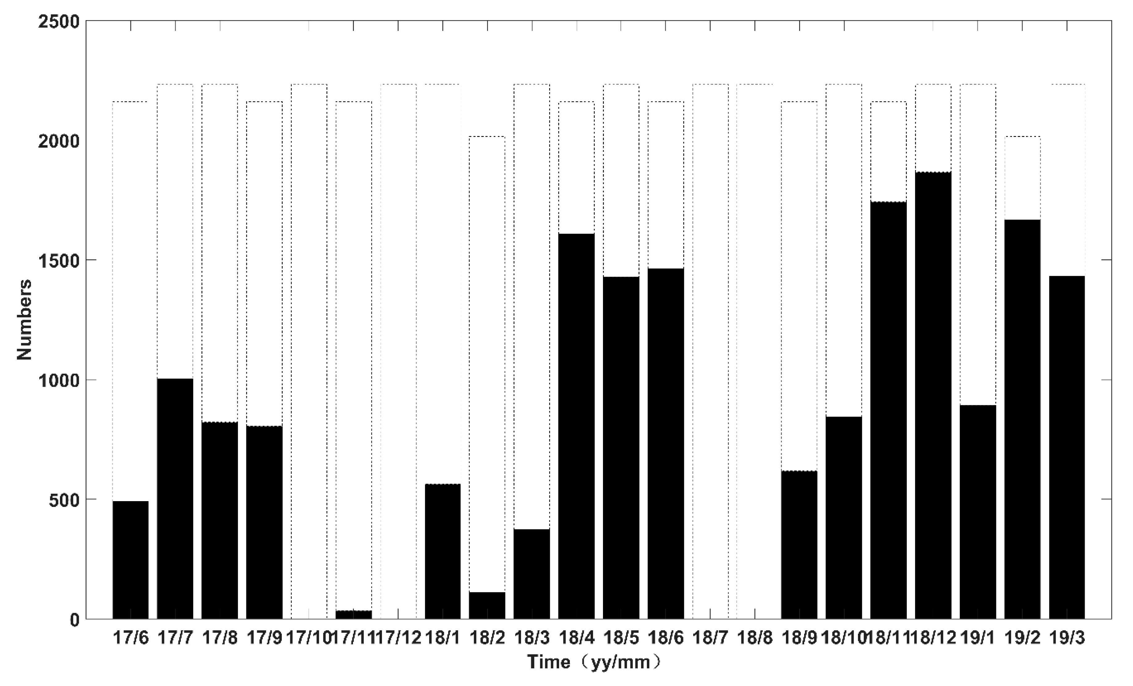
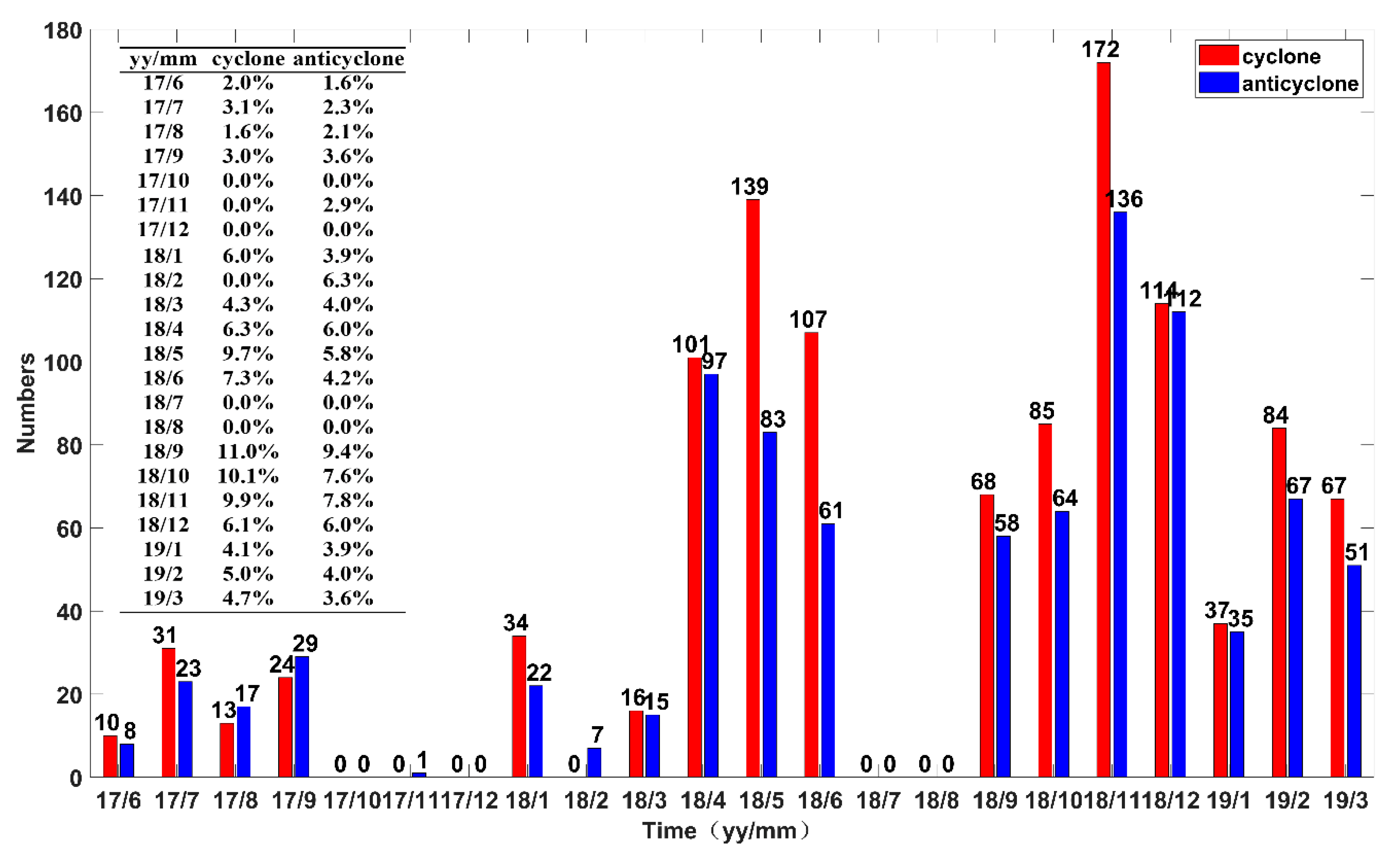
3.1. Features of Submesoscale Eddies (Eddy Properties) from HFR Observations

Submesoscale eddies were obtained from the HFR velocity fields, with a total of 1102 cyclonic eddies and 886 anticyclonic eddies identified, based on the VG eddy detection method. Submesoscale eddies cover most of the study region. Their number density is shown in Figure 6, which indicates that the occurrence of eddies mostly happens in the center of the study region and also in the southwestern coastal part. Moreover, the region where eddies frequently appear is off the cape at (39°40′N, 119°50′E) and the seamount in the center. In addition, a small number of eddies are detected in the study region as a result of being close to the outer edge of the HFR observation region. However, the identified eddies in the region do not show significant monthly variability due to differences in the validated data obtained each month (Figure 7).

The submesoscale characteristics have a radius of 1.3 to 8 km and an asymmetric normalized vorticity with a maximum between 0.3 and 1.5 (Figure 8). There is little difference between the size distribution of cyclonic and anticyclonic eddies. Figure 8 shows that eddies with a radius between 2 and 4 km are frequent, whereas eddies with a radius larger than 10 km are very infrequent. The mean radius values are 2.70 and 2.59 km for the anticyclonic and cyclonic eddies, respectively.

Table 1. Mean values of eddy kinematics.

	Mean	Std dev	Min	Max
Cyclonic eddies
Vorticity	2.84	1.97	0.31	9.92
Shearing deformation	0.30	1.46	−6.80	7.44
Stretching deformation	0.10	2.39	−11.94	10.42
Total deformation	2.13	2.14	0.16	13.34
Divergence	0.20	3.15	−15.20	15.40
Anticyclonic eddies
Vorticity	−3.30	2.06	−9.92	−0.25
Shearing deformation	−0.44	1.67	−7.73	5.31
Stretching deformation	0.32	2.52	−6.70	11.77
Total deformation	2.50	2.22	0.15	12.86
Divergence	0.25	3.36	−7.72	19.73

units: ${10}^{-5}{\mathrm{s}}^{-1}.$

lists the mean values of the eddies’ kinematic parameters. It illustrates that the average vorticity of anticyclonic eddies is larger than that of cyclonic eddies; moreover, the instability of anticyclonic eddies is also larger, according to the values of total deformation. Moreover, since surface current fields in this region are influenced by tides and topography, the vorticity of the surface current field is not large compared with western boundary region currents [45]. In addition, no significant difference is found for the radii of anticyclonic and cyclonic eddies.

3.2. Ability of Submesoscale Signals Extracted by CI-Derived Gradient Parameters

The CI-derived gradient parameters were calculated by the method described in Section 2. Figure 5 shows some examples of the gradient parameters at three different times. According to the location surrounded by the black dashed lines in Figure 3, the local CI is changed from large to small values. When anticyclonic eddies lasted for a short period, as shown in Figure 4, the anticyclonic eddies are found near the location of the black dashed lines in Figure 3; the size of anticyclonic eddies in the CI images is smaller than that from HFRs. In addition, a big difference is that there is one eddy that does exist in the center of HFR map and some other small eddies in this region. This illustrates that CI images could find the submesoscale signals due to physical processes, but they also contain other submesoscale information. The gradient parameters capture the submesoscale signals due to submesoscale anticyclonic eddies, and also other signals from other physical processes or biological processes. These processes mostly result from the sinking process accompanying anticyclonic eddies shown in Figure 3. The size and location of the anticyclonic eddies in CI gradient parameter fields have little difference from those in HFR-derived current fields because: (1) the Chl-a field aroused by the physical eddy field tends to be weaker than the current field and appears to be shifted by the force of the advection term; (2) the two datasets have different spatial resolutions and different properties (CI and velocity vectors). In addition, our method relies on a single image and gradient information, which is different from other studies about tracer-derived velocity products [46,47,48]. Nevertheless, some limitations do exist in both our method and the CI imagery when compared with HFR imagery. In fact, it is known in fluid mechanics that (a) submesoscale patterns could have taken a long time to emerge due to purely biological processes; (b) submesoscale patterns could be an example of “fossil turbulence” [49]. In both cases, the eddy patterns may only show up in the CI imagery as opposed to the HFR imagery. On the other hand, submesoscale eddies can exist without any color signature. Even with these known limitations, as long as eddy patterns are captured in the CI imagery, the CI-derived gradient parameters can successfully capture submesoscale signals.

Therefore, the CI-derived gradient parameters show similar eddy structures and provide even more submesoscale eddies. Although these gradient parameters do not provide realistic velocity fields, they are evidence of SPs and can also provide more detailed information about the eddy structures. This enhances the observation and analysis of submesoscale phenomena, implying that a CI (MODIS color pattern) with a resolution up to 500 m is a good tool to extract submesoscale signals from relatively larger observation areas, compared with HFR datasets.

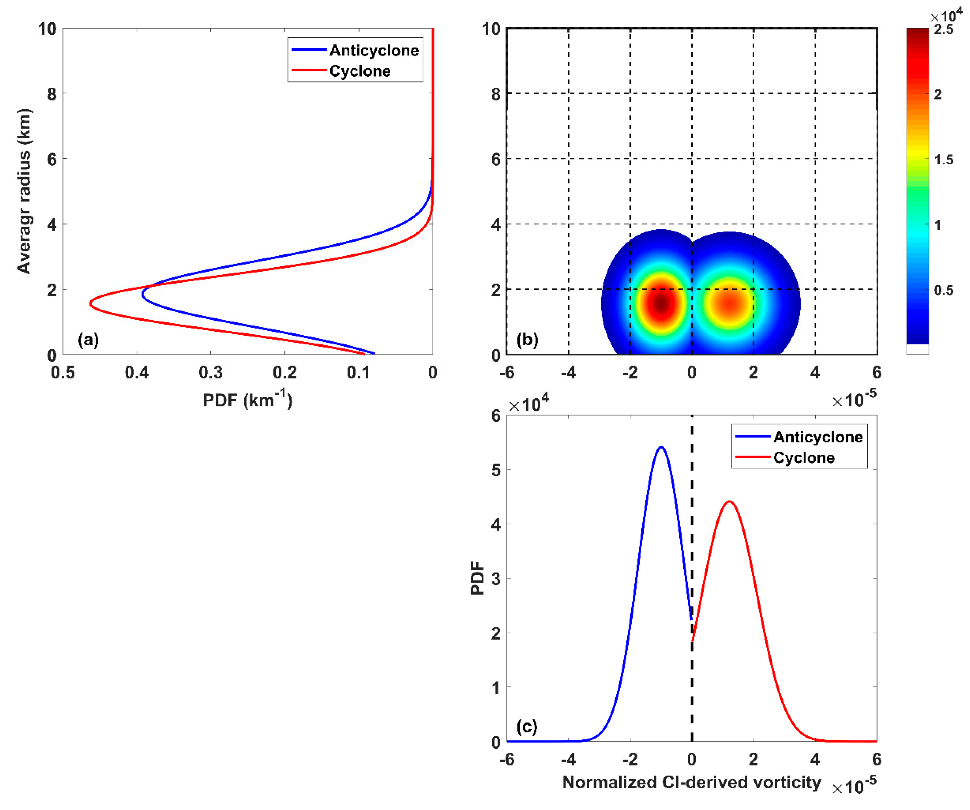
3.3. Characteristics of Submesoscale Eddies (Eddy Properties) from CI-derived Gradient Fields

The results indicate that more submesoscale eddies can be detected with MODIS CI patterns with a resolution of 500 m than with the HFR data with a resolution of 3 km, although the former have a much lower temporal frequency (i.e., at most once per day versus every 20 min from HFR). A total of 4990 anticyclonic eddies and 4968 cyclonic eddies were identified with the abovementioned eddy detection algorithm from CI-derived gradient fields, which is more than four times those identified from the HFR velocity fields. The monthly distribution of the number of anticyclonic and cyclonic eddies is shown in Figure 9. We don’t have sufficient CI data to report results during summer due to frequent clouds.

The CI-derived parameters (units: ${\mathrm{s}}^{-1}$) aren’t the actual velocities, and so the vorticity of the CI parameters only focuses on its relative value. In Figure 10a, the mean radius values for submesoscale eddies are 1.85 and 1.56 km for the anticyclonic and cyclonic eddies, respectively. The mean radius values are smaller than those computed by the HFR-derived eddies. This indicates that eddy structures with a higher resolution are more suitable to detect SPs, and therefore better able to observe submesoscale signals. The strength of anticyclonic and cyclonic eddies is almost equal, as shown in Figure 10c.

4. Discussion

The small sizes of the eddies detected from both HFR-derived currents and CI-derived gradient parameters are different from other coastal submesoscale eddies using HFRs [13,33]. Here, although eddies have high relative vorticities, they are weaker than the submesoscale island wake at Green Island in the Kuroshio, as simulated by Liu and Chang [45], who found that values for the eddy vorticity can reach up to $10f$ (f is the Coriolis parameter), and the wake exhibits frequently detached recirculation, containing upwelling and von Kármán vortex streets. In our study region, cyclonic (anticyclonic) eddies were often accompanied by an increase (decrease) in CI (representing Chl-a and other in-water constituents). Jang et al. [16] reported similar studies about eddy properties from HFRs but didn’t consider coastal responses of Chl-a because part of their study region did not have valid Geostationary Ocean Color Imager (GOCI) images. In this study, it is demonstrated that the efficient way to understand coastal SPs is via the application of HFR-derived currents and CI-derived gradient parameters.

The potential mechanism for the generation of submesoscale eddies in coastal areas can be inferred from geophysical factors, tides and wind stress. Firstly, a primary source for eddies’ generation consists of geophysical factors, including coastline changes and bottom topography. Topographic features, such as islands, headlands and seamounts, generally exhibit a turbulent–drag interaction between currents and the topography. The formation and separation of bottom boundary layers affects the generation and injection of vertical vorticity. In this study area, multiple regions of eddies are mainly located along the coastline and near the seamount. The seamount changes the local vorticity and thus increases the probability of submesoscale eddies. The current fields near the coastline become unstable due to lateral boundaries, which also contribute to the generation of submesoscale eddies. Secondly, eddy generation is one possible cause of asymmetric advection by the rotating tidal flow [5]. The major axis of the M2 semidiurnal current is ~29 cm/s near Lianyungang, which greatly influences the local currents. Thirdly, local eddies respond to the wind direction and the wind stress curl, thereby providing some indication of when and where eddies may be formed, evolve and ultimately dissipate [2]. Detailed discussions of these mechanisms will be presented in future papers, using numerical simulations.

In summary, although HFRs have some limitations due to their limited coastal coverage, they do meet the requirements for the spatio-temporal resolutions of SPs. Moreover, the gradient parameters derived from daily CI images have the ability to fill the gap left by HFRs, with the advantages of high space coverage. The latter method therefore shows potential for further research on SPs of global oceans.

5. Conclusions

In our study, CI-derived gradient parameters are calculated by a modified method from MODIS CI data. Two kinds of dataset, HFR-derived current fields and CI-derived gradient parameters, were applied to identify submesoscale eddies using the VG eddy detection algorithm, and thus to analyze the eddy properties. Both the HFR-derived velocity fields and the CI-derived gradient parameters are able to efficiently observe submesoscale eddies with data resolutions of 3 km and 500 m, respectively. The CI gradient parameters are able to capture more detailed submesoscale eddy features due to the higher spatial resolution of the CI images (500 m). However, the eddies’ distribution and sizes are found to have some differences because of different sampling rates, observational variables, response delay, fossil turbulence, and possibly colorless eddies. In conclusion, the study reveals that HFR surface currents and MODIS CI are good options to investigate SPs.

In the coastal Lianyungang region, a total of 1102 cyclonic eddies and 886 anticyclonic eddies were recorded from the HFR-derived velocity fields, and a total of 4990 anticyclonic eddies and 4968 cyclonic eddies were recorded from the MODIS CI-derived gradient parameters, based on the VG eddy detection algorithm. The typical radius of eddies derived from the HFR velocity fields was 2.70 and 2.59 km for the anticyclonic and cyclonic eddies, respectively. The typical radius of eddies derived from the CI images is slightly smaller than those found from the HFR velocity fields. Thus, an advantage of high-resolution data is that they can resolve the eddy structures in more detail.

This study is the first to extract submesoscale signals from MODIS CI data, with a resolution of 500 m, to investigate submesoscale coastal eddies. Comparing HFR surface currents with MODIS CI data, they can be mutually verified and they are complementary. Submesoscale eddies in CI images are detected near the location, where there are indeed some anticyclonic or cyclonic eddies from recent HFR records, revealing their consistency. So HFR data significantly prove the ability of submesoscale signals extracted from CI-derived gradient parameters, while CI data enhance the spatial resolution and the scope of the observations. Based on the VG eddy detection algorithm, submesoscale eddies near the coastal region of the Huang Sea, close to the city of Lianyungang, China have been well analyzed. This methodology is potentially useful for investigations of ecosystem distributions in coastal biological communities in other areas of the global ocean.

References

1. McWilliams, J.C. Submesoscale currents in the ocean. Proc. R. Soc. A 2016, 472, 32. [Google Scholar] [CrossRef] [PubMed]
2. Kirincich, A. The Occurrence, Drivers, and Implications of Submesoscale Eddies on the Martha’s Vineyard Inner Shelf. J. Phys. Oceanogr. 2016, 46, 2645–2662. [Google Scholar] [CrossRef]
3. Kim, S.Y.; Cornuelle, B.D.; Terrill, E.J. Decomposing observations of high-frequency radar-derived surface currents by their forcing mechanisms: Decomposition techniques and spatial structures of decomposed surface currents. J. Geophys. Res. 2010, 115. [Google Scholar] [CrossRef] [Green Version]
4. Du Plessis, M.; Swart, S.; Ansorge, I.J.; Mahadevan, A. Submesoscale processes promote seasonal restratification in the Subantarctic Ocean. J. Geophys. Res. 2017, 122, 2960–2975. [Google Scholar] [CrossRef]
5. Rocha, C.B.; Gille, S.T.; Chereskin, T.K.; Menemenlis, D. Seasonality of submesoscale dynamics in the Kuroshio Extension. Geophys. Res. Lett. 2016, 43, 304–311. [Google Scholar] [CrossRef]
6. Callies, J.; Ferrari, R.; Klymak, J.M.; Gula, J. Seasonality in submesoscale turbulence. Nat. Commun. 2015, 6, 6862. [Google Scholar] [CrossRef] [Green Version]
7. Thomas, L.N.; Tandon, A.; Mahadevan, A. Submesoscale processes and dynamics. Ocean Model. Eddy. Regime 2008, 17–38. [Google Scholar] [CrossRef] [Green Version]
8. Mahadevan, A.; Tandon, A. An analysis of mechanisms for submesoscale vertical motion at ocean fronts. Ocean Model. 2006, 14, 241–256. [Google Scholar] [CrossRef]
9. Tulloch, R.; Smith, K.S. A theory for the atmospheric energy spectrum: Depth-limited temperature anomalies at the tropopause. Proc. Natl. Acad. Sci. USA 2006, 103, 14690. [Google Scholar] [CrossRef] [Green Version]
10. Buckingham, C.E.; Naveira Garabato, A.C.; Thompson, A.F.; Brannigan, L.; Lazar, A.; Marshall, D.P.; George Nurser, A.J.; Damerell, G.; Heywood, K.J.; Belcher, S.E. Seasonality of submesoscale flows in the ocean surface boundary layer. Geophys. Res. Lett. 2016, 43, 2118–2126. [Google Scholar] [CrossRef] [Green Version]
11. D’Asaro, E.; Lee, C.; Rainville, L.; Harcourt, R.; Thomas, L. Enhanced Turbulence and Energy Dissipation at Ocean Fronts. Science 2011, 332, 318. [Google Scholar] [CrossRef] [PubMed] [Green Version]
12. Haza, A.C.; Özgökmen, T.M.; Griffa, A.; Molcard, A.; Poulain, P.-M.; Peggion, G. Transport properties in small-scale coastal flows: Relative dispersion from VHF radar measurements in the Gulf of La Spezia. Ocean Dyn. 2010, 60, 861–882. [Google Scholar] [CrossRef]
13. Kim, S.Y. Observations of submesoscale eddies using high-frequency radar-derived kinematic and dynamic quantities. Cont. Shelf Res. 2010, 30, 1639–1655. [Google Scholar] [CrossRef]
14. Lekien, F.; Coulliette, C. Chaotic stirring in quasi-turbulent flows. Philos. Trans. R. Soc. A 2007, 365, 3061–3084. [Google Scholar] [CrossRef]
15. Shcherbina, A.Y.; D’Asaro, E.A.; Lee, C.M.; Klymak, J.M.; Molemaker, M.J.; McWilliams, J.C. Statistics of vertical vorticity, divergence, and strain in a developed submesoscale turbulence field. Geophys. Res. Lett. 2013, 40, 4706–4711. [Google Scholar] [CrossRef]
16. Yoo Jang, G.; Kim Sung, Y.; Kim Hyeon, S. Spectral Descriptions of Submesoscale Surface Circulation in a Coastal Region. J. Geophys. Res. 2018. [Google Scholar] [CrossRef]
17. Kim, S.Y.; Terrill, E.J.; Cornuelle, B.D.; Jones, B.; Washburn, L.; Moline, M.A.; Paduan, J.D.; Garfield, N.; Largier, J.L.; Crawford, G.; et al. Mapping the U.S. West Coast surface circulation: A multiyear analysis of high-frequency radar observations. J. Geophys. Res. 2011, 116. [Google Scholar] [CrossRef] [Green Version]
18. Lai, Y.; Zhou, H.; Yang, J.; Zeng, Y.; Wen, B. Submesoscale Eddies in the Taiwan Strait Observed by High-Frequency Radars: Detection Algorithms and Eddy Properties. J. Atmos. Ocean. Technol. 2017, 34, 939–953. [Google Scholar] [CrossRef]
19. Soh, H.S.; Kim, S.Y. Diagnostic Characteristics of Submesoscale Coastal Surface Currents. J. Geophys. Res. 2018, 123, 1838–1859. [Google Scholar] [CrossRef]
20. Choi, J.-K.; Park, Y.J.; Ahn, J.H.; Lim, H.-S.; Eom, J.; Ryu, J.-H. GOCI, the world’s first geostationary ocean color observation satellite, for the monitoring of temporal variability in coastal water turbidity. J. Geophys. Res. 2012, 117. [Google Scholar] [CrossRef]
21. Garfield, N.; Hubbard, M.; Pettigrew, J. Providing SeaSonde high-resolution surface currents for the America’s Cup. In Proceedings of the 2011 IEEE/OES 10th Current, Waves and Turbulence Measurements (CWTM), Monterey, CA, USA, 20–23 March 2011; pp. 47–49. [Google Scholar]
22. Pomales-Velázquez, L.; Morell, J.; Rodriguez-Abudo, S.; Canals, M.; Capella, J.; Garcia, C. Characterization of mesoscale eddies and detection of submesoscale eddies derived from satellite imagery and HF radar off the coast of southwestern Puerto Rico. In Proceedings of the OCEANS 2015-MTS/IEEE Washington, Monterey, CA, USA, 19–22 October 2015; pp. 1–6. [Google Scholar]
23. Hu, J.; Wang, X.H. Progress on upwelling studies in the China seas. Rev. Geophys. 2016, 54, 653–673. [Google Scholar] [CrossRef]
24. Huang, W.; Wang, W.; Zhang, W.; Zhang, J. Analysis of Characteristics of the Tides and the Tidal Currents in Adjacent Waters of Lianyungang Port. Zhejiang Hydrotech. 2012, 3, 1–5. [Google Scholar] [CrossRef]
25. Chavanne, C.; Flament, P.; Gurgel, K.-W. Interactions between a Submesoscale Anticyclonic Vortex and a Front. J. Phys. Oceanogr. 2010, 40, 1802–1818. [Google Scholar] [CrossRef] [Green Version]
26. Jeong, J.; Hussain, F. On the identification of a vortex. J. Fluid Mech. 1995, 285, 69–94. [Google Scholar] [CrossRef]
27. Sadarjoen, I.A.; Post, F.H. Geometric Methods for Vortex Extraction. In Proceedings of the Data Visualization ’99, Vienna, Austria, 26–28 May 1999; pp. 53–62. [Google Scholar]
28. Chaigneau, A.; Pizarro, O. Eddy characteristics in the eastern South Pacific. J. Geophys. Res. 2005, 110. [Google Scholar] [CrossRef]
29. McWilliams, J.C. The vortices of two-dimensional turbulence. J. Fluid Mech. 1990, 219, 361–385. [Google Scholar] [CrossRef]
30. Morrow, R.; Donguy, J.-R.; Chaigneau, A.; Rintoul, S.R. Cold-core anomalies at the subantarctic front, south of Tasmania. Deep Sea Res. Part I 2004, 51, 1417–1440. [Google Scholar] [CrossRef]
31. Ari Sadarjoen, I.; Post, F.H. Detection, quantification, and tracking of vortices using streamline geometry. Comput. Graph. 2000, 24, 333–341. [Google Scholar] [CrossRef]
32. Sadarjoen, I.A.; Post, F.H.; Bing, M.; Banks, D.C.; Pagendarm, H. Selective visualization of vortices in hydrodynamic flows. In Proceedings of the Visualization ‘98 (Cat. No.98CB36276), Triangle Park, NC, USA, 18–23 October 1998; pp. 419–422. [Google Scholar]
33. Nencioli, F.; Dong, C.; Dickey, T.; Washburn, L.; McWilliams, J.C. A Vector Geometry–Based Eddy Detection Algorithm and Its Application to a High-Resolution Numerical Model Product and High-Frequency Radar Surface Velocities in the Southern California Bight. J. Atmos. Ocean. Technol. 2010, 27, 564–579. [Google Scholar] [CrossRef]
34. Heiberg, E.; Ebbers, T.; Wigstrom, L.; Karlsson, M. Three-dimensional flow characterization using vector pattern matching. IEEE Trans. Vis. Comput. Graph. 2003, 9, 313–319. [Google Scholar] [CrossRef]
35. Ebling, J.; Scheuermann, G. Clifford convolution and pattern matching on vector fields. In Proceedings of the IEEE Visualization, VIS 2003, Seattle, WA, USA, 19–24 October 2003; pp. 193–200. [Google Scholar]
36. Chaigneau, A.; Gizolme, A.; Grados, C. Mesoscale eddies off Peru in altimeter records: Identification algorithms and eddy spatio-temporal patterns. Prog. Oceanogr. 2008, 79, 106–119. [Google Scholar] [CrossRef]
37. Dong, C.; Nencioli, F.; Liu, Y.; McWilliams, J.C. An Automated Approach to Detect Oceanic Eddies From Satellite Remotely Sensed Sea Surface Temperature Data. IEEE Geosci. Remote Sens. Lett. 2011, 8, 1055–1059. [Google Scholar] [CrossRef]
38. Hu, C. An empirical approach to derive MODIS ocean color patterns under severe sun glint. Geophys. Res. Lett. 2011, 38. [Google Scholar] [CrossRef]
39. Liu, Y.Y.; Weisberg, R.H.R.H.; Hu, C.C.; Kovach, C.C.; RiethmüLler, R.R. Evolution of the Loop Current System During the Deepwater Horizon Oil Spill Event as Observed with Drifters and Satellites. Monit. Modeling Deep. Horiz. Oil Spill 2011, 195, 91–101. [Google Scholar]
40. Zhang, Y.; Hu, C.; Liu, Y.; Weisberg, R.H.; Kourafalou, V.H. Submesoscale and Mesoscale Eddies in the Florida Straits: Observations from Satellite Ocean Color Measurements. Geophys. Res. Lett. 2019, 46, 13262–13270. [Google Scholar] [CrossRef]
41. Sobel, I.; Feldman, G. A 3 × 3 Isotropic Gradient Operator for Image Processing. In Pattern Classification and Scene Analysis; Duda, R., Hart, P., Eds.; John Wiley & Sons: Stanford, CA, USA, 1968; pp. 271–272. [Google Scholar]
42. Dong, C.; Mavor, T.; Nencioli, F.; Jiang, S.; Uchiyama, Y.; McWilliams, J.C.; Dickey, T.; Ondrusek, M.; Zhang, H.; Clark, D.K. An oceanic cyclonic eddy on the lee side of Lanai Island, Hawai’i. J. Geophys. Res. 2009, 114. [Google Scholar] [CrossRef] [Green Version]
43. Liu, Y.; Dong, C.; Guan, Y.; Chen, D.; McWilliams, J.; Nencioli, F. Eddy analysis in the subtropical zonal band of the North Pacific Ocean. Deep Sea Res. Part I 2012, 68, 54–67. [Google Scholar] [CrossRef]
44. Ji, J.; Dong, C.; Zhang, B.; Liu, Y.; Zou, B.; King, G.P.; Xu, G.; Chen, D. Oceanic Eddy Characteristics and Generation Mechanisms in the Kuroshio Extension Region. J. Geophys. Res. 2018, 123, 8548–8567. [Google Scholar] [CrossRef]
45. Liu, C.-L.; Chang, M.-H. Numerical Studies of Submesoscale Island Wakes in the Kuroshio. J. Geophys. Res. 2018. [Google Scholar] [CrossRef]
46. Yang, H.; Choi, J.-K.; Park, Y.-J.; Han, H.-J.; Ryu, J.-H. Application of the Geostationary Ocean Color Imager (GOCI) to estimates of ocean surface currents. J. Geophys. Res. 2014, 119, 3988–4000. [Google Scholar] [CrossRef]
47. Crocker, R.I.; Matthews, D.K.; Emery, W.J.; Baldwin, D.G. Computing Coastal Ocean Surface Currents From Infrared and Ocean Color Satellite Imagery. IEEE Trans. Geosci. Remote Sens. 2007, 45, 435–447. [Google Scholar] [CrossRef]
48. Kozlov, I.E.; Artamonova, A.V.; Manucharyan, G.E.; Kubryakov, A.A. Eddies in the Western Arctic Ocean From Spaceborne SAR Observations Over Open Ocean and Marginal Ice Zones. J. Geophys. Res. 2019, 124, 6601–6616. [Google Scholar] [CrossRef] [Green Version]
49. Leung, P.-T.; Gibson, C.H. Turbulence and fossil turbulence in oceans and lakes. Chin. J. Oceanol. Limnol. 2004, 22, 1–23. [Google Scholar] [CrossRef]
Figure 1. (a) The Google satellite image near Lianyungang, China. The region of the color image is the coverage region of Moderate Resolution Imaging Spectroradiometer (MODIS) color patterns. The region of the black solid frame is the coverage region of High-Frequency coastal Radars (HFRs) (90.8 × 66.7 km); (b) The bathymetry of the study area (units: m). The background color shows the topography. The black contours are the isobaths, which show the 3, 10, and 20 m bathymetric contours. The black dots are vector points derived from the HFRs. The two green triangles are the locations of the two HFRs. The bathymetry data is from Global Ocean and Land Terrain Models’ (GEBCO’s) gridded bathymetric dataset, which is a global terrain model for ocean and land at 15 arc-second intervals.
Remotesensing 12 00711 g001
Figure 2. Number of HFR-derived surface current field records for each month. The data are recorded once every 20 min. Shaded areas indicate the number of data for each month.
Remotesensing 12 00711 g002
Figure 3. Three examples of MODIS color index (CI) fields at (a) 0535 UTC on 10 Jul 2017, (b) 0440 UTC on 11 Jul 2017 and (c) 0525 UTC on 12 Jul 2017. The submesoscale anticyclonic eddies are indicated by the black dashed lines. The values on the legend represent the relative magnitudes of CI, with higher values indicating more turbid waters. Note that, for the three days shown here, MODIS Chl-a images do not show valid data in most areas.
Remotesensing 12 00711 g003
Figure 4. Examples of the eddy detection algorithm. Surface current velocity fields are obtained with HFRs at (a) 11:40 UTC on 10 July 2017 and (b) 12:40 UTC on 10 July 2017. The blue solid lines are eddy boundaries and the blue dots are centers of anticyclonic eddies, both estimated from the vector geometry (VG) method.
Remotesensing 12 00711 g004
Figure 5. Examples of CI-derived gradient fields at (a) 0535 UTC on 10 Jul 2017, (b) 0440 UTC on 11 July 2017 and (c) 0525 UTC on 12 July 2017. Vectors are derived from the CI patterns. The blue (red) dots and solid lines are anticyclonic (cyclonic) eddy centers and boundaries identified by the VG method. Values on the legend represent relative magnitudes of CI. Higher values indicate more turbid waters.
Remotesensing 12 00711 g005
Figure 6. The total number of cyclonic (a) and anticyclonic (b) eddies derived by HFRs current fields based on the VG method during the observation period. The total number of eddies in each grid is increased if the eddy exists in the grid.
Remotesensing 12 00711 g006
Figure 7. Histogram of the monthly distribution of eddies identified by HFR-derived current fields. The table shows the ratio of the cyclonic (anticyclonic) eddy number to the total observation records each month.
Remotesensing 12 00711 g007
Figure 8. Probability density functions (PDFs) of the various characteristics of the identified submesoscale eddies from HFR-derived velocity fields. (a,c): 1-D PDFs for radius and vorticity; (b): joint PDF for radius vorticity.
Remotesensing 12 00711 g008
Figure 9. Histogram of the monthly distribution of eddies identified by CI-derived gradient parameters.
Remotesensing 12 00711 g009
Figure 10. Probability density functions (PDFs) of the various characteristics of the identified submesoscale eddies from the CI-derived parameters. (a,c), 1-D PDFs for radius and vorticity; (b), joint PDF of radius vorticity.
Remotesensing 12 00711 g010