Training Data Selection for Annual Land Cover Classification for the Land Change Monitoring, Assessment, and Projection (LCMAP) Initiative

Abstract

The U.S. Geological Survey’s Land Change Monitoring, Assessment, and Projection (LCMAP) initiative involves detecting changes in land cover, use, and condition with the goal of producing land change information to improve the understanding of the Earth system and provide insights on the impacts of land surface change on society. The change detection method ingests all available high-quality data from the Landsat archive in a time series approach to identify the timing and location of land surface change. Annual thematic land cover maps are then produced by classifying time series models. In this paper, we describe the optimization of the classification method used to derive the thematic land cover product. We investigated the influences of auxiliary data, sample size, and training from different sources such as the U.S. Geological Survey’s Land Cover Trends project and National Land Cover Database (NLCD 2001 and NLCD 2011). The results were evaluated and validated based on independent data from the training dataset. We found that refining the auxiliary data effectively reduced artifacts in the thematic land cover map that are related to data availability. We improved the classification accuracy and stability considerably by using a total of 20 million training pixels with a minimum of 600,000 and a maximum of 8 million training pixels per class within geographic windows consisting of nine Analysis Ready Data tiles (450 by 450 km²). Comparisons revealed that the NLCD 2001 training data delivered the best classification accuracy. Compared to the original LCMAP classification strategy used for early evaluation (e.g., Trends training data, 20,000 samples), the optimized classification strategy improved the annual land cover map accuracy by an average of 10%.

1. Introduction

Land cover and land change play a major role in the climate and biogeochemistry of the Earth system [1]. Remote sensing has long been used as an effective tool for broad-scale land cover mapping [2]. As a result, many land cover datasets have been developed with resolutions ranging from 1 km to 30 m e.g., [1,3,4]. The U.S. Geological Survey (USGS) has a long history of characterizing land cover using moderate spatial resolution remote sensing data to support regional and national assessments for both science and management [4,5]. The USGS National Land Cover Database (NLCD) has produced 30-m land cover products since 1992 [3,6,7,8]. Currently, NLCD is being updated every 2–3 years for the conterminous U.S. and every 10 years for Alaska. Driven by concerns about climate change and resource sustainability [9,10], land cover product needs are expanding due to the demand for increasingly innovative and timely land cover and land change inquiries. The USGS response to this growing need is the Land Change Monitoring, Assessment, and Projection (LCMAP) initiative [11].

LCMAP utilizes recently released U.S. Landsat Analysis Ready Data (ARD) [12] to characterize historical changes in land cover, use, and condition from 1985 to 2017. The ARD product comprises surface reflectance data over the United States from the Thematic Mapper (Landsats 4 and 5), Enhanced Thematic Mapper Plus (ETM+) (Landsat 7), and Operational Land Imager (Landsat 8) [12]. Landsat ARD is structured with a 150 x 150 km tile scheme and uses the Albers Equal Area Conic projection. From the ARD data, LCMAP derives annual land cover maps using an adaptation of the Continuous Change Detection and Classification (CCDC) algorithm [13,14]. The CCDC algorithm uses all cloud-free observations in a time series of ARD to detect change in a specific pixel location based on the spectral and temporal properties of the land surface. The algorithm then classifies a pixel before and after a detected change using random forest [15].

The quest to provide better land cover classification results has driven the development and exploration of many classification methods. Machine-learning classification algorithms, such as the artificial neural network, support vector machine, and random forest, have recently drawn more attention in remote sensing e.g., [16,17,18]. Compared with traditional classification methods, machine learning can effectively handle large dimensional training data and complex data spaces [19]. However, like other supervised classification approaches, the training data for machine learning play an essential role in classification accuracy [20]. Optimizing machine-learning training data often includes four aspects: (1) feature selection; (2) the amount of training data; (3) the distribution of training data among the classes; and (4) the balance of training data among the classes. A feature in machine-learning is defined as an individual property or characteristic that can be used to distinguish land cover classes. Multiple studies have suggested that the selection of appropriate features can significantly improve classification accuracy e.g., [21,22] because feature selection is directly related to the separability of classes. The training data size is usually positively correlated to the classification accuracy because a large set of training data can better represent class variation. But the distribution and balancing of training data among classes are also crucial in machine-learning classification [23]. Distribution refers to the proportion of training data for a specific class, which is often related to the population of the map classes in the study area [15]. In contrast, balance refers to the population difference between the dominant class and minor classes. The classification approaches usually optimize the overall accuracy, while points in minority classes or subclasses with a small sample size might be considered as outliers and ignored.

The initial CCDC classification strategy was designed based on five Landsat path/rows across the conterminous United States (CONUS), with training data from map products of the USGS Land Cover Trends project [15]. The strategy suggested (1) extracting training data based on the proportional occurrence of land cover classes with a total of 20,000 pixels; (2) balancing larger and smaller classes by using a minimum of 600 and a maximum of 8000 training pixels for each class; and (3) including eight auxiliary variables to improve the classification accuracy (aspect, elevation, positional index, slope, Wetland Potential Index, water probability, snow probability, and cloud probability). The overall accuracy improved from 80% to 88% when applying the optimized strategy.

This paper presents the lessons learned in optimizing the classification procedure for the operational and automated generation of annual land cover maps. We applied the CCDC algorithm to Landsat ARD and evaluated land cover maps at 24 tiles across CONUS [11]. Overall, the land cover maps matched well with Trends, NLCD, and Google Earth high-resolution imagery. However, the study identified some issues, including Landsat 7 ETM+ Scan Line Corrector (SLC) effects occurring in data prior to the SLC failure, and the occasional misclassification of small towns or barren land cover that were not well represented in the training data. We hypothesized that the first issue was related to static auxiliary layers that failed to represent the 30-year dynamics, while the second issue indicated that more training data are necessary to represent within-class variations (e.g., different types of barren land cover or different densities of developed areas). In this study, we optimized the land cover classification strategy by refining some auxiliary layers and increasing the training data. Because the Trends data have limited national coverage, we explored NLCD land cover products as our training data. We conducted the optimization study focusing on the following questions:

(1) Do the auxiliary data cause spatial patterns indicative of the SLC-off effect to be found in outputs prior to the SLC failure?

(2) What is the optimum amount of training data?

(3) What is the optimum source of training data?

2. Data and Study Area

2.1. Landsat Analysis Ready Data (ARD)

Collection 1 Landsat ARD [12] from 1982 to 2017 was acquired as the initial input for CCDC. The product is processed to 5000 × 5000 30-m pixel (150 × 150 km) tiles in the Albers Equal Area Conic projection, a modified tile scheme of the CONUS Web-Enabled Landsat Data (WELD) products [24]. The acquired ARD product includes seven surface reflectance bands, brightness temperatures, and pixel quality assessments (QA) from Landsats 4, 5, 7, and 8. We filtered out pixels that were labeled as cloud or cloud shadow in the pixel QA band. The details of clouds and cloud shadow filtering are discussed in Zhu, Gallant, Woodcock, Pengra, Olofsson, Loveland, Jin, Dahal, Yang and Auch [15].

2.2. LCMAP Continuous Change Detection

LCMAP applied the CCDC algorithm on the ARD surface reflectance bands to estimate the time series models and detect land surface changes at the pixel scale [13,14]. Each time series model represents a period of stable land cover, and the coefficients of the model delineate the spectral and temporal variation of the pixel (Equation (1)). The time series models are used by CCDC as inputs for the land cover classification, which includes the harmonic coefficients, slope, intercept, and root mean square error. This study uses the same model components as CCDC, except we adjusted the intercept of the model coefficients (c_0,i) to the center of the model (c_0,i + c_1,it_center). The adjusted value aims to better characterize the overall spectra of the model than the intercept (estimated spectra on January 1 at year 1).

$$\widehat{\rho }\left(i,t\right)=c_{0,i}+c_{1,i}t+{\displaystyle \sum }_{n=1}^3{a}_{n,i}cos\frac{2\pi t}{L}+b_{n,i}sin\frac{2\pi t}{L}$$

(1)

where $\widehat{\rho }\left(i,t\right)$ is the predicted value for the i_th Landsat band at the Julian date t. $c_{0,i}$ and $c_{1,i}$ are the estimated intercept and slope coefficients for the i_th Landsat band, respectively, while $a_{n,i}$ and $b_{n,i}$ are the estimated n_th order seasonal harmonic coefficients for the i_th Landsat band. L is the length of cycles, i.e., the number of days per year.

2.3. Auxiliary Data

The CCDC classification strategy used three groups of static auxiliary layers [15]: probability layers derived from the Landsat pixel QA band, topographic layers, and the Wetland Potential Index (WPI). The Landsat pixel QA band stores information about the cloud, water, and snow occurrence for each Landsat observation, from which the probability layers were calculated as the percentage of cloud, water, or snow in the entire time series. For example, the cloud probability layer represents the percentage of cloud-contaminated observations in the whole time series for each pixel. The topographic layers and WPI were also used by NLCD [7,15]. The topographic layers were calculated from the National Elevation Dataset (NED), including the elevation, aspect, slope, and Positional Index (PI) [25]. The WPI was developed based on NLCD 2006, National Wetlands Inventory [26], and Soil Survey Geographic Database (SSURGO) for hydric soils [27].

2.4. National Land Cover Database (NLCD)

NLCD 2001 and 2011 were selected as training source candidates because of their national wall-to-wall coverage. Also, NLCD is a widely used and well-established land cover dataset derived from Landsat. Though NLCD recently released a new suite of products that offered seven integrated epochs of land cover for the years 2001, 2003, 2006, 2008, 2011, 2013, and 2016 [7,28,29], this study was conducted before the new data release. We used the previous NLCD data release, which included land cover products for 2001, 2006, and 2011. Using NLCD 2001 as the baseline, NLCD mapped 16 land cover classes (Anderson Level II) in the native 30-m × 30-m resolution at 5-year intervals (2001, 2006, and 2011). We selected NLCD 2001 and 2011 because 2001 was in the middle of the time series, while 2011 represented the latest evolution of NLCD products at the time of this study [7]. The overall accuracies of the two products were 83% and 82% at Level II and 89% and 88% at Level I for 2001 and 2011, respectively [30]. The LCMAP land cover legend is similar to the Anderson Level I [5] and includes a total of eight classes: Developed, Cropland, Tree Cover, Grass/Shrub, Wetland, Water, Ice/Snow, and Barren. We cross-walked NLCD land cover maps to match the LCMAP class scheme (

Table 1. The cross-walk from National Land Cover Database (NLCD) to Land Change Monitoring, Assessment, and Projection (LCMAP) classes. The values in parentheses are the NLCD land cover class code.

NLCD class	LCMAP class
Water (11)	Water
Perennial ice/snow (12)	Ice and Snow
Developed, open space (21)	Developed
Developed, low intensity (22)	Developed
Developed, medium intensity (23)	Developed
Developed, high intensity (24)	Developed
Barren (31)	Barren
Deciduous forest (41)	Tree Cover
Evergreen forest (42)	Tree Cover
Mixed forest (43)	Tree Cover
Shrubland (52)	Grass/shrub
Grassland (71)	Grass/shrub
Pasture (81)	Cropland
Cultivated crops (82)	Cropland
Woody wetlands (90)	Wetland
Herbaceous wetland (95)	Wetland

). Zhu et al. [15] previously suggested that removing spectral and spatial outliers contained in the Trends training data had no significant improvement in classification results. However, we found that the cross-walked NLCD classes could mismatch with ARD images at the embedded road network and class edges because of the projection difference. The NLCD embedded road network had increased misclassifications in the initial tests because many of the embedded road pixels were mixed and dominated by a class other than Developed. Thus, NLCD classes were eroded by one pixel.

2.5. Study Area

Eight ARD tiles were selected to capture different land cover types and ecosystems across CONUS (selected tiles are indicated by orange squares in Figure 1). The eight tiles were located within six sites that were previously evaluated using 2 × 2 blocks of ARD tiles [11]. We selected the eight tiles to fully depict challenges in the evaluation sites and to reduce the optimization time. The six sites represented a variety of landscapes, land change scenarios, and data richness (

Table 2. Land cover percentage (%) in the eight Landsat Analysis Ready Data (ARD) tiles derived from the cross-walked National Land Cover Database (NLCD) 2011.

Tile	Developed	Cropland	Grass/Shrub	Tree	Water	Wetland	Snow Ice	Barren
H03V09	1.5	2.4	47.3	39.0	2.1	0.4	0	7
H03V10	6.0	33.1	28.6	21.9	0.8	0.3	0	4.8
H05V02	3.2	36.5	47.1	6.7	2.9	1.1	0	0
H05V03	4.6	44.7	37.4	10.2	1.6	0.5	0	0
H13V06	2.0	5.8	71.0	12.9	0.5	1.5	0	5.5
H20V15	6.9	8.7	13.6	47.1	2.3	11.9	0	0.2
H21V08	17.6	69.7	1.8	4.4	2.7	1.4	0	0.2
H28V08	27.5	18.1	2.7	19.3	11.8	9.4	0	0.3

).

3. Methods

The initial implementation of CCDC used the random forest classifier, which was computationally intensive and not reasonable for the production of broad-scale land cover mapping. As a result, we switched to a newly developed classifier, XGBoost [31]. The XGBoost classifier is optimized for handling big data via parallel processing, caching intermediate results, and building small individual decision trees. The new classifier has been found to produce similar quality results to other classification approaches, including random forest, and the differences are small compared to the importance of appropriate training data [32,33]. The format of XGBoost results is also the same as random forest in that probabilities are associated with each land cover label. After time series models were classified, we used the land cover class on July 1 of each year to generate annual maps, which is the same approach as the initial CCDC methodology [15]. For periods following a disturbance where a new model was not immediately established, we filled the disturbance with the previous land cover type if the period was before the "disturbance" day or with the latter land cover type if the period was after the "disturbance" day. Five main LCMAP cover products (primary cover, secondary cover, primary confidence, secondary confidence, and land cover change) were mapped, representing the most likely and the second most likely land cover type associated with their probabilities and the primary land cover change from the prior year to the current year. This study built on the CCDC classification strategy [15] and focused on (1) refining auxiliary data, (2) optimizing the sample size of training data, and (3) selecting the best training data source.

3.1. Auxiliary Data Refining

We focused on the probability layers in the auxiliary data because (1) these layers were static and did not depict climate variations through the 33 years (i.e., 1985–2017), and (2) these layers spread the problem related to post-2003 SLC-off data to the whole time series. In this test, we removed the probability layers while leaving the rest of the classification strategy to be the same as for the initial version of CCDC. We then compared the results at problematic sites that were previously identified to evaluate the impacts of the probability layers.

3.2. Training Sample Size Optimization

We trained each ARD tile using NLCD 2001 from the surrounding 3 × 3 tiles. We then tested maximum sample sizes ranging from 20K, 200K, 2M, 20M, to 100M pixels using a stratified random selection based on the proportion of classes. The proportion-based stratified random sampling is considered better than simple random sampling [15,34], especially for small urban areas [11]. The CCDC classification strategy used a maximum of 8000 pixels for each class to keep classes balanced, with a maximum total of 20K samples. In this study, we followed the strategy but scaled up the minimum and maximum boundaries according to the total sample size. Because of the class balance constraint, the actual sample size could be less than the maximum sample size when only a few classes dominated the ARD tile. Each test scenario was conducted 10 times to estimate the stability of the classification scenario.

We used 80% of the training samples to build the classification model and 20% to evaluate the model. We evaluated the agreement between the model prediction and the 20% training samples and referred to this agreement as "accuracy" [15]. The log loss (Equation (2)) was used to evaluate the models, and is commonly applied in machine-learning optimization [31]. Log loss is considered a better indicator than the simple agreement assessment in model evaluation because the simple agreement only measures how often a predicted value equals the actual value while log loss also rates the uncertainty of predictions:

$$L_{\log }\left(y,p\right)=-\log \mathrm{Pr}(y|p)=-\left(y \log \left(p\right)+\left(1-y\right)\log \left(1-p\right)\right)$$

(2)

where y is a binary indicator of the actual class, and p is the model probability for the corresponding class. Pr represents a likelihood function that delineates how confident the model is in the actual class. If we convert the probabilities to binary by assigning the highest probability to 1 and the rest to 0, the Pr would be equivalent to the simple agreement. In most cases, the Pr or log loss incorporates not only the correctness of the classification but also the model probability to the correct class. For a better interpolation, we used the Pr as the criterion and considered it to be the classification accuracy.

Moreover, the land cover consistency through iteration was also evaluated as a criterion. The consistency analysis compared land cover maps from eight iterations and recorded the number of different classes that occurred in each pixel. We used eight iterations out of 10 because eight was the maximum possible number of different classes that could occur in a pixel. The consistency analysis was also conducted using different training sizes for Trends data, which indicated the stability of the original CCDC classification strategy. However, since Trends data did not have 20M pixels in 3 × 3 tiles, only 20K, 200K, and 2M sample sizes were used.

3.3. Training Data Source Optimization

Alternative sampling strategies included a single era of NLCD data (NLCD 2001 or NLCD 2011), a combination of two NLCD eras (NLCD 2001&2011), and NLCD 2001 excluding Pasture/Hay (i.e., NLCD 2001 no Pasture/Hay). The last sampling strategy was designed to investigate whether Pasture/Hay is more similar to Cropland or to Grass/Shrub using the current classification inputs. The classification of Pasture/Hay is often challenging because it is usually covered by grasses but is used for livestock grazing or hay cropping, which causes it to be spectrally similar to grass, but it is an agricultural practice with a similar disturbance cycling to cropland.

The evaluation of the data source is based on accuracy comparison and visual comparison. The first three scenarios (NLCD 2001, NLCD 2011, and NLCD 2001&2011) were run 10 times to estimate the stability of the accuracy comparison. The last scenario was run only once in each tile for the visual comparison only. To provide a qualitative but rigorous evaluation of different sources of training data, six members of the LCMAP team with land cover experience evaluated the classification products based on the CCDC classification (Trends-based) and the four NLCD-based alternatives. Interpreters were chosen from geographers and land cover scientists at the USGS Earth Resources Observation and Science (EROS) Center who possessed an average of 17 years of experience with a combination of previous and current USGS land cover projects, including the Global Land Cover Characterization [4], Land Cover Trends, and NLCD, in addition to LCMAP. Interpreters were aware of the sampling methodologies used, but identifications of the five alternatives were masked to reduce interpreter bias. Four LCMAP cover products (primary cover, secondary cover, primary confidence, and secondary confidence) for 1984–2017 were provided to interpreters along with a variety of metrics quantifying the agreement with NLCD and earlier results. The 1984 LCMAP results were also evaluated by interpreters, though the maps were not included in the final LCMAP products. Interpreters largely focused on primary cover maps in their evaluations. Six tiles were selected, one from each evaluation region: H03V09, H05V02, H13V06, H20V15, H21V08, and H28V08. Five of the interpreters focused on two tiles each, and one interpreter focused on one tile (H20V15 was evaluated by only one interpreter, the others by two interpreters). At the time of the evaluations, the results from Trends and NLCD 2011 training were not available for H20V15, H21V08, and H28V08; interpreters evaluated the three available alternatives for these tiles. Each interpreter independently evaluated the alternatives, followed by a group discussion of all interpreters to synthesize perspectives and select preferred alternative(s).

4. Results and Discussion

4.1. Auxiliary Data Refining

The impact of the probability layers was examined by comparing the classification results at a problematic area (Figure 2). New Melones Lake in California is a reservoir surrounded by a hilly area composed of trees and grass. Figure 2a illustrates the strips of tree cover in the CCDC version of the land cover map in 1995. Because the probability layers were derived from 33 years of Landsat QA bands, some SLC-off artifacts from these probability layers were propagated back in time into results prior to the SLC failure. The strips disappeared when the probability layers were removed while leaving the rest of the classification strategy the same (Figure 2b), although more pixels were classified as trees. This test suggested that though machine-learning methods automatically select the most useful features for classification, inputting reliable and representative features is still important for the classification [35]. Thus, we removed the three auxiliary data layers from the LCMAP algorithm.

4.2. Training Sample Size Optimization

The comparison of the overall accuracies based on the different training sample sizes showed the accuracy increasing along with the training sample size for all eight tiles, and the accuracy variation (standard deviation) decreasing as well (

Table 3. The overall accuracy for a total of 20K, 200K, 2M, 20M, and 100M stratified training samples from National Land Cover Database (NLCD) 2001. The standard deviation is calculated from the accuracy through 10 iterations.

Tile	20K		200K		2M		20M		100M
	Accuracy	STD	Accuracy	STD	Accuracy	STD	Accuracy	STD	Accuracy	STD
H03V09	0.84	0.0135	0.89	0.0025	0.92	0.0007	0.94	0.0002	0.94	0.0001
H03V10	0.83	0.0130	0.88	0.0022	0.91	0.0006	0.94	0.0002	0.94	0.0001
H05V02	0.85	0.0105	0.88	0.0022	0.91	0.0009	0.93	0.0002	0.93	0.0001
H05V03	0.84	0.0070	0.89	0.0029	0.91	0.0005	0.94	0.0002	0.94	0.0000
H13V06	0.79	0.0097	0.85	0.0026	0.89	0.0008	0.91	0.0002	0.93	0.0001
H20V15	0.84	0.0052	0.88	0.0022	0.90	0.0008	0.92	0.0002	0.93	0.0001
H21V08	0.78	0.0102	0.83	0.0023	0.86	0.0006	0.90	0.0002	0.93	0.0001
H28V08	0.80	0.0137	0.83	0.0024	0.86	0.0010	0.89	0.0002	0.91	0.0001

). The initial strategy had an accuracy of less than 85%, while increased training data improved the accuracy by about 10%. The accuracy of the initial strategy was consistent with the CCDC results (80%-88%) that used the same sample size but a different training data source and classifier. The accuracy improvements gradually saturated after 0.91, except for two tiles (H21V08 and H28V08) that show accuracy continuing to improve with the increasing training data. The two tiles also had a lower accuracy than the other tiles in all the training sample size tests. Figure 3 illustrates the sample distributions across all classes in relation to the maximum per class population. The horizontal lines in the first row suggest that some minor classes reached the maximum population in the training data after 200K or 2M. Thus, further increasing training data did not benefit those minor classes but increased the imbalance among classes. We did not use the paired t-test to estimate the significance of accuracy improvements [15] because the extensive training data consistently produced significant results with less than a 1% improvement across iterations using this test. Computation time needs to be considered along with accuracy so that the LCMAP products can be generated and updated in a reasonable time frame. The time costs rose exponentially with an increasing training sample size (

Table 4. The time cost (hour) of generating a classification model for 20K, 200K, 2M, 20M, and 100M stratified training samples.

Tile	20K	200K	2M	20M	100M
H03V09	0.04	0.06	0.25	2.62	11.54
H03V10	0.04	0.05	0.24	2.36	10.33
H05V02	0.04	0.06	0.35	3.25	13.90
H05V03	0.04	0.06	0.32	3.08	13.84
H13V06	0.04	0.05	0.20	1.97	8.06
H20V15	0.04	0.05	0.23	2.81	13.27
H21V08	0.05	0.06	0.28	2.23	9.90
H28V08	0.04	0.05	0.30	2.86	13.02

), despite the saturation of the accuracy improvement (Table 3). The average time to generate one classification model was much less than 1 hour when the total training sample size was 2M or less but increased to 2 and 10 hours for 20M and 100M training samples, respectively (based on 20 CPUs, 3.00 Ghz). Additionally, not all tiles could collect 100M training samples. For example, tile H13V06 was dominated by grass/shrub, while all other classes were relatively minor. So, to maintain the proportion of classes, the stratified random selection only collected a total of 48,689,930 samples for the 100M tests, which also led to less time cost (Table 4).

Figure 4 shows an example of the consistency measurements across iterations. The value, from 1 to 8, indicated the number of different classes that occurred in the eight iterations of classification. The region, located at Lake McClure, California, was mostly covered by grass with sparse trees along the water body and in the hilly area at the northeast side of the lake. Most of the pixels with inconsistent results came from the tree-grass mixed area, and the pixels with the most class variations were around the edge between water and land. The NLCD-based results generally delivered fewer inconsistent pixels than the Trends-based results for the same training data size (Figure 4). The number of inconsistent pixels decreased with the increase of training data from either Trends or NLCD. The improvements also occurred at the tile scale and were steady through the time series (Figure 5). The red dotted line in Figure 5 represents the consistency of the initial strategy that could be improved by 15% with additional training data. However, the consistency improvements were also saturated with increased training data. A similar relationship between the consistency and sample size was also found using random forest [36]. Based on the above analysis, a total of 20M training data samples with a minimum of 60,000 and a maximum of 8M pixels for each class was used.

4.3. Training Data Source Optimization

All interpreters agreed that the NLCD-based land cover had a substantially higher quality than the Trends-based CCDC results. The most noted example was that large areas of clear development (e.g., Rapid City, South Dakota) were not classified as Developed in the original land cover [11]. In general, interpreters found boundaries between areas of differing land cover to be sharper for the NLCD-based alternatives, with less mixing of land cover and fewer misclassified isolated pixels.

Interpreters differed in which of the NLCD eras they preferred. For five of the six evaluations of the three western tiles (H03V09, H05V02, and H13V06), interpreters selected NLCD 2001 as the preferred option (NLCD 2001&2011 was preferred by one interpreter for H13V06). For the three eastern tiles, the preferences were more mixed, with one interpreter giving a slight edge to NLCD 2001 for two tiles (H20V15 and H21V08), another interpreter expressing equal preference between NLCD 2001 and NLCD 2001&2011 for the Illinois tile (H21V08), and two interpreters preferring NLCD 2001&2011 for the Chesapeake tile (H28V08). Despite the knowledge that one of the alternatives focused on Pasture/Hay training, interpreters generally found little to distinguish between NLCD 2001 and NLCD 2001 no Pasture/Hay. All interpreters who selected NLCD 2001 as their preferred training alternative expressed a roughly even preference between NLCD 2001 and NLCD 2001 no Pasture/Hay.

The model accuracies from 10 iterations of different training data sources were above 0.88 for all classifications (Figure 6). The ranges of accuracies were less than 0.001 across 10 iterations. The results derived from NLCD 2001 consistently outperformed the results based on NLCD 2011 at eight tiles. NLCD 2001 and NLCD 2001&2011 derived a similar accuracy at the H03V10 tile, but NLCD 2001 outperformed at four out of eight tiles, while NLCD 2001&2011 outperformed at three out of eight tiles. Thus, NLCD 2001 was selected as the final training data source. Although the NLCD 2011 land cover map is derived from the NLCD 2001 product with land cover change updates, the accuracy of the NLCD 2011 land cover map is slightly lower than the NLCD 2001 map [30]. Thus, NLCD 2001 was selected as the source for LCMAP training data. Other advantages of NLCD 2001 that were considered were the conceptual clarity of utilizing a single year of data with no excluded classes, and the fact that training based on 2001 would be closer in time to all the dates in the 1985–2017 time period.

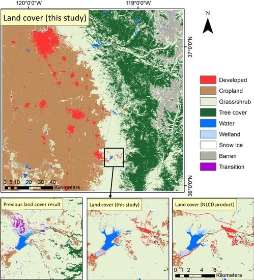
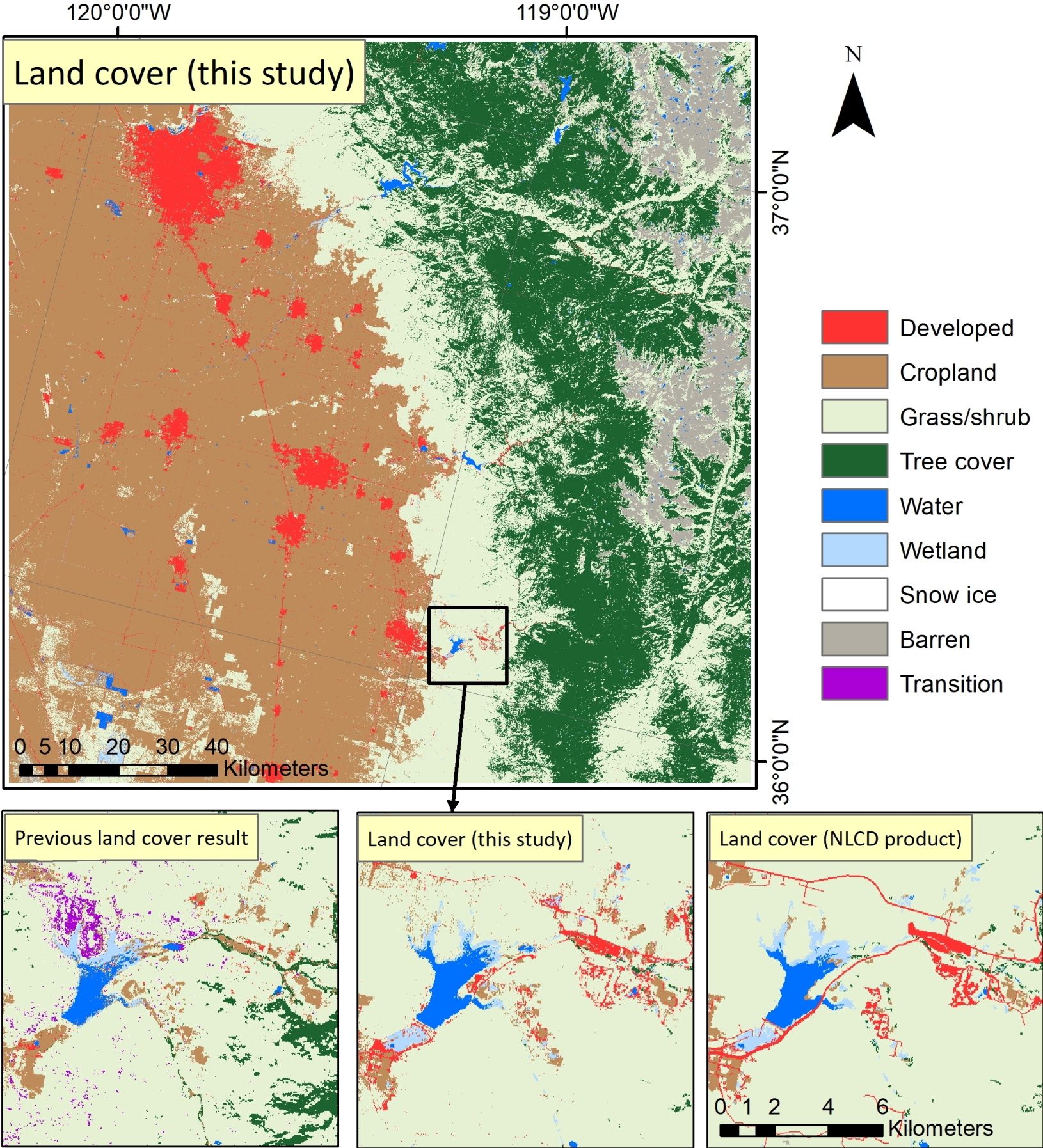
4.4. Comparison of Classification Results After the Optimization

Finally, Figure 7a shows optimized classification results in the southern California area. The zoomed-in panels show the differences between the original CCDC classification results (Figure 7b) and the optimized results from this study (Figure 7c) in the Lake Success area of California. The purple class in the original CCDC map means a disturbance occurred where a new model was not immediately established on July 1. In the recent LCMAP results, the class was filled with the previous land cover type if the period was before the "disturbance" day and with the latter land cover type if the period was after the "disturbance" day [11]. Compared to the cross-walked NLCD (Figure 7d), the original CCDC failed to identify some developed areas such as the Springville Valley in the eastern part of Figure 7b. The area southwest of Lake Success was classified as cropland in Figure 7b, while Figure 7c,d showed this area as wetland. Moreover, Figure 7b found more tree cover than Figure 7c,d.

5. Conclusions

In this study, we sought to improve the land cover classification data products that are part of the LCMAP initiative. We optimized multiple aspects (e.g., auxiliary data, training sample size, and training data source) of the operational automated land cover mapping of the conterminous United States within the LCMAP initiative. We removed three auxiliary data layers from the classification feature set that were derived from the Landsat quality band because these static layers spread data artifacts throughout the time series. We selected NLCD 2001 as the training data source and increased the total training data sample to 20M. The Trends dataset was designed to describe land changes across the U.S., but its block sampling strategy was not representative of minor land cover classes or classes with high within-class variability. The final classification strategy for LCMAP includes three steps. (1) A total of 20M training data points are extracted based on the proportional occurrence of land cover classes. (2) The training data are balanced by using a minimum of 600,000 and a maximum of 8M training pixels for each class. (3) Five auxiliary data layers (aspect, elevation, positional index, slope, and Wetland Potential Index) are used as input features. We adapted the recently developed XGBoost classifier to improve computation time. However, the results of this study suggest that the classifier inputs such as feature selection and appropriate, representative training data are more important to the land cover classification than algorithm selection. This LCMAP classification strategy is a foundation for characterizing land cover and detecting land change as it occurs. The strategy may be modified when other features, training data sources, or land cover legends are used, but the methodology of optimization can still be applied.

References

1. Friedl, M.A.; McIver, D.K.; Hodges, J.C.; Zhang, X.Y.; Muchoney, D.; Strahler, A.H.; Woodcock, C.E.; Gopal, S.; Schneider, A.; Cooper, A. Global land cover mapping from MODIS: Algorithms and early results. Remote Sens. Environ. 2002, 83, 287–302. [Google Scholar] [CrossRef]
2. Chen, J.; Chen, J.; Liao, A.; Cao, X.; Chen, L.; Chen, X.; He, C.; Han, G.; Peng, S.; Lu, M. Global land cover mapping at 30 m resolution: A POK-based operational approach. Isprs J. Photogramm. Remote Sens. 2015, 103, 7–27. [Google Scholar] [CrossRef] [Green Version]
3. Homer, C.; Dewitz, J.; Fry, J.; Coan, M.; Hossain, N.; Larson, C.; Herold, N.; McKerrow, A.; VanDriel, J.N.; Wickham, J. Completion of the 2001 national land cover database for the counterminous United States. Photogramm. Eng. Remote Sens. 2007, 73, 337. [Google Scholar]
4. Loveland, T.R.; Reed, B.C.; Brown, J.F.; Ohlen, D.O.; Zhu, Z.; Yang, L.; Merchant, J.W. Development of a global land cover characteristics database and IGBP DISCover from 1 km AVHRR data. Int. J. Remote Sens. 2000, 21, 1303–1330. [Google Scholar] [CrossRef]
5. Anderson, J.R. A land use and land cover classification system for use with remote sensor data; US Government Printing Office: Washington, DC, USA, 1976; Volume 964. [Google Scholar]
6. Fry, J.A.; Xian, G.; Jin, S.; Dewitz, J.A.; Homer, C.G.; Yang, L.; Barnes, C.A.; Herold, N.D.; Wickham, J.D. Completion of the 2006 national land cover database for the conterminous United States. Photogramm. Eng. Remote Sens. 2011, 77, 858–864. [Google Scholar]
7. Homer, C.; Dewitz, J.; Yang, L.; Jin, S.; Danielson, P.; Xian, G.; Coulston, J.; Herold, N.; Wickham, J.; Megown, K. Completion of the 2011 National Land Cover Database for the conterminous United States–representing a decade of land cover change information. Photogramm. Eng. Remote Sens. 2015, 81, 345–354. [Google Scholar]
8. Vogelmann, J.E.; Sohl, T.L.; Campbell, P.; Shaw, D. Regional land cover characterization using Landsat Thematic Mapper data and ancillary data sources. Environ. Monit. Assess. 1998, 51, 415–428. [Google Scholar] [CrossRef]
9. Rindfuss, R.R.; Walsh, S.J.; Turner, B.L.; Fox, J.; Mishra, V. Developing a science of land change: Challenges and methodological issues. Proc. Natl. Acad. Sci. USA 2004, 101, 13976–13981. [Google Scholar] [CrossRef] [Green Version]
10. Turner, B.L.; Lambin, E.F.; Reenberg, A. The emergence of land change science for global environmental change and sustainability. Proc. Natl. Acad. Sci. USA 2007, 104, 20666–20671. [Google Scholar] [CrossRef] [Green Version]
11. Brown, J.F.; Tollerud, H.J.; Barber, C.P.; Zhou, Q.; Dwyer, J.; Vogelmann, J.E.; Loveland, T.; Woodcock, C.E.; Stehman, S.V.; Zhu, Z. Lessons learned implementing an operational continuous United States national land change monitoring capability: The Land Change Monitoring, Assessment, and Projection (LCMAP) approach. Remote Sens. Environ. 2020, 111356. [Google Scholar] [CrossRef]
12. Dwyer, J.; Roy, D.; Sauer, B.; Jenkerson, C.; Zhang, H.; Lymburner, L. Analysis ready data: Enabling analysis of the Landsat archive. Remote Sens. 2018, 10, 1363. [Google Scholar]
13. Zhu, Z.; Woodcock, C.E.; Holden, C.; Yang, Z. Generating synthetic Landsat images based on all available Landsat data: Predicting Landsat surface reflectance at any given time. Remote Sens. Environ. 2015, 162, 67–83. [Google Scholar] [CrossRef]
14. Zhu, Z.; Woodcock, C.E. Continuous change detection and classification of land cover using all available Landsat data. Remote Sens. Environ. 2014, 144, 152–171. [Google Scholar] [CrossRef] [Green Version]
15. Zhu, Z.; Gallant, A.L.; Woodcock, C.E.; Pengra, B.; Olofsson, P.; Loveland, T.R.; Jin, S.; Dahal, D.; Yang, L.; Auch, R.F. Optimizing selection of training and auxiliary data for operational land cover classification for the LCMAP initiative. Isprs J. Photogramm. Remote Sens. 2016, 122, 206–221. [Google Scholar] [CrossRef] [Green Version]
16. Huang, C.; Davis, L.; Townshend, J. An assessment of support vector machines for land cover classification. Int. J. Remote Sens. 2002, 23, 725–749. [Google Scholar] [CrossRef]
17. Ma, L.; Liu, Y.; Zhang, X.; Ye, Y.; Yin, G.; Johnson, B.A. Deep learning in remote sensing applications: A meta-analysis and review. Isprs J. Photogramm. Remote Sens. 2019, 152, 166–177. [Google Scholar] [CrossRef]
18. Rani, S.; Dhingra, S. REVIEW ON SATELLITE IMAGE CLASSIFICATION BY MACHINE LEARNING AND OPTIMIZATION APPROACHES. Int. J. Adv. Res. Comput. Sci. 2017, 8. [Google Scholar] [CrossRef]
19. Mountrakis, G.; Im, J.; Ogole, C. Support vector machines in remote sensing: A review. Isprs J. Photogramm. Remote Sens. 2011, 66, 247–259. [Google Scholar] [CrossRef]
20. Millard, K.; Richardson, M. On the importance of training data sample selection in random forest image classification: A case study in peatland ecosystem mapping. Remote Sens. 2015, 7, 8489–8515. [Google Scholar] [CrossRef] [Green Version]
21. Liu, H.; Dougherty, E.R.; Dy, J.G.; Torkkola, K.; Tuv, E.; Peng, H.; Ding, C.; Long, F.; Berens, M.; Parsons, L. Evolving feature selection. Ieee Intell. Syst. 2005, 20, 64–76. [Google Scholar] [CrossRef]
22. Salehi, M.; Sahebi, M.R.; Maghsoudi, Y. Improving the accuracy of urban land cover classification using Radarsat-2 PolSAR data. Ieee J. Sel. Top. Appl. Earth Obs. Remote Sens. 2013, 7, 1394–1401. [Google Scholar]
23. Mellor, A.; Boukir, S.; Haywood, A.; Jones, S. Exploring issues of training data imbalance and mislabelling on random forest performance for large area land cover classification using the ensemble margin. Isprs J. Photogramm. Remote Sens. 2015, 105, 155–168. [Google Scholar] [CrossRef]
24. Roy, D.P.; Ju, J.; Kline, K.; Scaramuzza, P.L.; Kovalskyy, V.; Hansen, M.; Loveland, T.R.; Vermote, E.; Zhang, C. Web-enabled Landsat Data (WELD): Landsat ETM+ composited mosaics of the conterminous United States. Remote Sens. Environ. 2010, 114, 35–49. [Google Scholar] [CrossRef]
25. Gesch, D.; Oimoen, M.; Greenlee, S.; Nelson, C.; Steuck, M.; Tyler, D. The national elevation dataset. Photogramm. Eng. Remote Sens. 2002, 68, 5–32. [Google Scholar]
26. Wilen, B.O.; Bates, M. The US fish and wildlife service’s national wetlands inventory project. In Classification and inventory of the world’s wetlands; Springer: Berlin, Germany, 1995; pp. 153–169. [Google Scholar]
27. Soil Survey Staff. Natural Resources Conservation Service; United States Department of Agriculture: Washington, DC, USA, 2008. Available online: https://websoilsurvey.nrcs.usda.gov/ (accessed on 3 August 2016).
28. Jin, S.; Homer, C.; Yang, L.; Danielson, P.; Dewitz, J.; Li, C.; Zhu, Z.; Xian, G.; Howard, D. Overall Methodology Design for the United States National Land Cover Database 2016 Products. Remote Sens. 2019, 11, 2971. [Google Scholar] [CrossRef] [Green Version]
29. Yang, L.; Jin, S.; Danielson, P.; Homer, C.; Gass, L.; Bender, S.M.; Case, A.; Costello, C.; Dewitz, J.; Fry, J. A new generation of the United States National Land Cover Database: Requirements, research priorities, design, and implementation strategies. Isprs J. Photogramm. Remote Sens. 2018, 146, 108–123. [Google Scholar] [CrossRef]
30. Wickham, J.; Stehman, S.V.; Gass, L.; Dewitz, J.A.; Sorenson, D.G.; Granneman, B.J.; Poss, R.V.; Baer, L.A. Thematic accuracy assessment of the 2011 national land cover database (NLCD). Remote Sens. Environ. 2017, 191, 328–341. [Google Scholar] [CrossRef] [Green Version]
31. Chen, T.; Guestrin, C. Xgboost: A scalable tree boosting system. In Proceedings of the 22nd acm sigkdd international conference on knowledge discovery and data mining, San Francisco, CA, USA, 13–17 August 2016; pp. 785–794. [Google Scholar]
32. Freeman, E.A.; Moisen, G.G.; Coulston, J.W.; Wilson, B.T. Random forests and stochastic gradient boosting for predicting tree canopy cover: Comparing tuning processes and model performance. Can. J. For. Res. 2015, 46, 323–339. [Google Scholar] [CrossRef] [Green Version]
33. Maxwell, A.E.; Warner, T.A.; Fang, F. Implementation of machine-learning classification in remote sensing: An applied review. Int. J. Remote Sens. 2018, 39, 2784–2817. [Google Scholar] [CrossRef] [Green Version]
34. Jin, H.; Stehman, S.V.; Mountrakis, G. Assessing the impact of training sample selection on accuracy of an urban classification: A case study in Denver, Colorado. Int. J. Remote Sens. 2014, 35, 2067–2081. [Google Scholar] [CrossRef]
35. Hall, M.A.; Smith, L.A. Practical feature subset selection for machine learning. In Computer Science ’98, Proceedings of the 21st Australasian Computer Science Conference ACSC’98, Perth, Astralia, 4–6 February 1998; McDonald, C., Ed.; Springer: Berlin, Germany, 1998; pp. 1716–1741. [Google Scholar]
36. Scornet, E.; Biau, G.; Vert, J.-P. Consistency of random forests. Ann. Stat. 2015, 43, 1716–1741. [Google Scholar] [CrossRef]
37. National Agriculture Imagery Program (NAIP). Information Sheet. 2013. Available online: https://www.fsa.usda.gov/Internet/FSA_File/naip_info_sheet_2013.pdf (accessed on 29 April 2019).
Figure 1. Landsat Landsat Analysis Ready Data (ARD) tiling scheme for the conterminous United States. The orange tiles show the locations of evaluation sites used in the preliminary Land Change Monitoring, Assessment, and Projection (LCMAP) evaluation. These tiles were selected to represent different land cover types and ecosystems across the conterminous Unites States (CONUS).
Remotesensing 12 00699 g001
Figure 2. Example of the classification problem in 1995 at New Melones Lake, California (38021.26”N, 1203319.20”W). Panel (a) shows the Landsat 7 ETM+ Scan Line Corrector (SLC) off strip effect using the original Continuous Change Detection and Classification (CCDC) classification strategy. Panel (b) shows the result with probability layers removed from the CCDC classification strategy.
Remotesensing 12 00699 g002
Figure 3. The pixel distribution of each class in comparative relation to the class upper limits (8000, 80,000, 800,000, 8,000,000, and 40,000,000, respectively) for a total of 20K, 200K, 2M, 20M, and 100M stratified training samples.
Remotesensing 12 00699 g003
Figure 4. The top row shows the consistency map from National Land Cover Database (NLCD) 2001–based 2010 land cover results, which were derived from eight iterations with up to 100M training data samples. The second row shows the consistency from Trends-based 2010 land cover results with up to 2M training samples (18 km × 18 km, Lake McClure, California. 373539.04”N, 1201544.65”W). The bottom row shows the location in a high-resolution image [37] and NLCD 2011 [7].
Remotesensing 12 00699 g004
Figure 5. The proportion of tile H03V09 that has consistent results through eight iterations of classification for a total of 20K, 200K, 2M, 20M, and 100M stratified National Land Cover Database (NLCD) 2001 samples.
Remotesensing 12 00699 g005
Figure 6. The average accuracy distribution of 10 iterations at 8 tiles using training data from National Land Cover Database (NLCD) 2001 and 2011, and 2001&2011. The standard deviation of accuracy across 10 iterations was less than 0.001 for all tests.
Remotesensing 12 00699 g006
Figure 7. Demonstration of the classification results at the southern California site: (a) land cover result from this study, (b) close up of the Lake Success area land cover using the Continuous Change Detection and Classification (CCDC) classification strategy, (c) close up of the land cover result based on this study, and (d) cross-walked 2011 National Land Cover Database (NLCD) land cover for comparison.
Remotesensing 12 00699 g007