Angle Distance-Based Hierarchical Background Separation Method for Hyperspectral Imagery Target Detection

Abstract

Traditional detectors for hyperspectral imagery (HSI) target detection (TD) output the result after processing the HSI only once. However, using the prior target information only once is not sufficient, as it causes the inaccuracy of target extraction or the unclean separation of the background. In this paper, the target pixels are located by a hierarchical background separation method, which explores the relationship between the target and the background for making better use of the prior target information more than one time. In each layer, there is an angle distance (AD) between each pixel spectrum in HSI and the given prior target spectrum. The AD between the prior target spectrum and candidate target ones is smaller than that of the background pixels. The AD metric is utilized to adjust the values of pixels in each layer to gradually increase the separability of the background and the target. For making better discrimination, the AD is calculated through the whitened data rather than the original data. Besides, an elegant and ingenious smoothing processing operation is employed to mitigate the influence of spectral variability, which is beneficial for the detection accuracy. The experimental results of three real hyperspectral images show that the proposed method outperforms other classical and recently proposed HSI target detection algorithms.

1. Introduction

A hyperspectral remote sensing system uses sensors to collect the energy reflected by ground materials in a wide electromagnetic band range, producing hyperspectral imagery (HSI) with abundant spectral information [1,2]. HSI is a data cube with one spectral dimension and two spatial dimensions. Each pixel in HSI corresponds to a spectral vector, which can reflect its material characteristic and provide the basis for analysis in HSI [3]. Target detection (TD), as an important part in the HSI processing field, is applied in both civil and military communities [4,5].

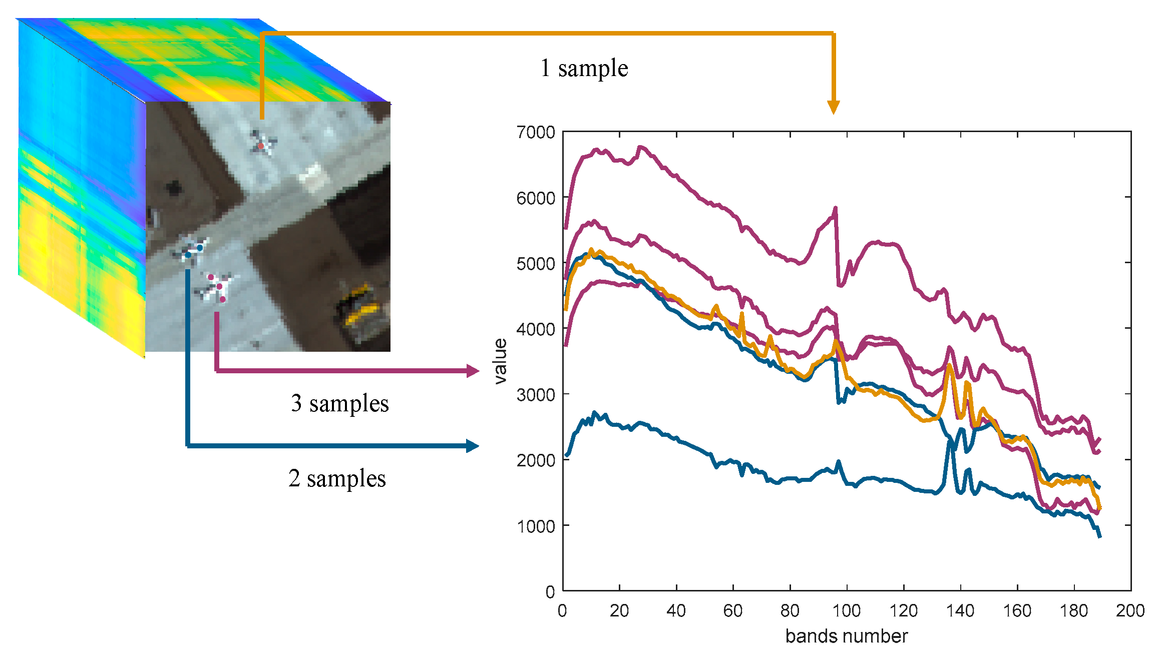
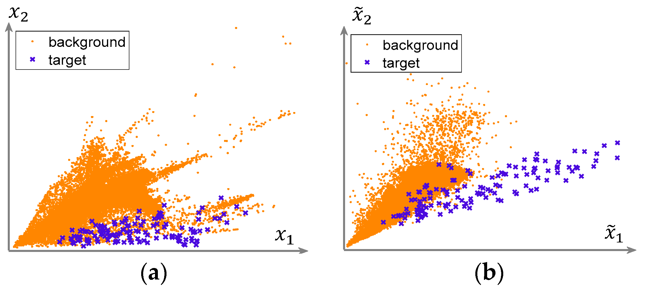
Different materials have unique spectral characteristics, thus spectral information plays a critical role in the TD field. Generally, whether two materials belong to the same category depends on the consistency of their spectra under the case without both interference and spectral aliasing. In the ideal assumption, the TD task in HSI will become extremely simple, because the main work can be concentrated on judging the consistency of two spectral vectors. However, the situation in real scenes is far from this assumption, as shown in Figure 1. Although six samples in the HSI are chosen from the same type of aircraft projected, even the same one, differences in their spectral curves still exist. The intrinsic reason lies in diverse interference factors, such as the noise in the imaging device, unideal electromagnetic wave transmission environment, and reflection surface, as well as the aliasing between adjacent but different materials. All of these interferences cause variability in spectra, and make the problem of TD more challenging [3,6,7].

To simplify the TD problem, researchers commonly divide the pixels in HSI into two parts: Targets of interest and backgrounds of indifference. Given this, the TD problem is described by a binary hypothesis model, which consists of two hypotheses: H₀ (target absent) and H₁ (target present) [8,9,10].

Some models have been proposed to reasonably describe spectral variability for better solving of the TD task. The probability density model is widely used in the TD field, which supposes that the spectra of each species obey the Gauss distribution. Many classical TD algorithms are derived according to this model, such as matched filter (MF) [3], spectral matched filter (SMF) [11], and adaptive coherence estimator (ACE) [12,13]. These methods assume that the background pixels have the same covariance structure but different means under two hypotheses, and adopt the generalized likelihood ratio test (GLRT) [14]. Subspace models are also widely used to explicate the phenomenon of variety [3]. They suppose that the spectrum vectors vary in a subspace of the band space, where the dimensions of the band space are equal to the length of the spectral vector. Based on the above assumptions, the matched subspace detector (MSD) [15], adaptive subspace detector (ASD) [12,16], and orthogonal subspace projection (OSP) [17,18] detector identify targets through the projection of the spectral vectors of tested pixels in a subspace. Unlike the above algorithms, the spectral angle mapper (SAM) [19] distinguishes targets from backgrounds by measuring the angle distance (AD). Furthermore, the constrained energy minimization (CEM) algorithm employs a finite impulse response (FIR) filter with a constraint, which minimizes the output energy while preserving the target [4,20]. A robust detection algorithm uses an inequality constraint on CEM (CEM-IC) based on the spectral variability rather than the equality constraint in CEM [21]. These methods have simple structures and can be easily implemented; however, they are accompanied with strict assumptions, and the utilization of target information is insufficient. Therefore, the TD results are often not accurate enough.

Recently, numerous TD methods have adopted machine learning-related technology. The kernel method is applied in many classical algorithms, and has also been used to produce kernel-based detectors, including kernel SMF, kernel MSD, kernel OSP, and kernel ASD [1,22]. These methods exploit higher-order statistics rather than using the first- and second-order statistics, and provide crucial information about data by the implicit exploitation of nonlinear features in the manner of a kernel. Furthermore, techniques about low-rank matrices and sparse representation are also employed in the TD field. The sparsity-based target detector (STD) [23,24] and the sparse representation-based binary hypothesis (SRBBH) [25] express a pixel by a linear combination of very few atoms from an overcomplete dictionary consisting of targets and backgrounds. Additionally, the detector based on low-rank and sparse matrix decomposition (LRaSMD) [26,27] utilizes the low-rank property of backgrounds and the sparse property of targets. In addition, multitask learning (MLT) is also used in target detection [28,29]. Besides, some methods combining the sparsity and other structured or unstructured detectors have been proposed, like the hybrid sparsity and statistics detector (HSSD) [30], the hybrid sparsity and distance-based discrimination (HSDD) detector [31], the sparse CEM, and the sparse ACE [32]. The above methods take advantage of some of the properties in HSI, but they often use a complex optimization algorithm to solve related object functions, which is more time consuming than traditional and classical methods.

One method for the TD problem, whether it is the classical method or the latest method proposed based on new technologies, relies on the prior spectra to locate targets, thus it is very significant to acquire one or more accurate and representative target spectra. If we randomly select several target samples as the input, the test results will appear fluctuated and biased [33]. The existence of the interfering factors mentioned above is an obstacle to finding a satisfactory spectrum. Recently, some scholars have studied this problem and have proposed various methods, such as the extracting method-based endmember extraction (EE) [34,35], adaptive weighted learning method using a self-completed background dictionary (AWLM_SCBD) [36], and target signature optimization based on sparse representation [33]. These methods improve the accuracy of detection results by finding more accurate target spectra.

Moreover, there is another issue that is easily neglected; that is, how to make better use of the known prior information of the target, which is also an important factor affecting the detection performance, and which is what we are concentrating on in our work. At present, few people analyze the TD problem in HSI from this perspective. Due to the existence of spectral variation, there is often no significant demarcation line between the target and the background pixels. However, it is reasonable to make full use of spectral information to enhance the separability between them. Recently, Zou et al. [37] proposed a hierarchical CEM (hCEM) algorithm as an improvement of CEM, greatly improving the detection accuracy of the latter. The hCEM builds hierarchical architecture to suppress the backgrounds spectra while preserving the targets. This method overcomes the deficiency of CEM, which is that it cannot completely suppress the backgrounds in one round of the filtering process. In hCEM, the prior target spectrum is used more than one time, so we can see that the hCEM makes better use of prior target information than CEM, and that is why hCEM outperforms CEM. However, when the backgrounds are suppressed by the hCEM algorithm, some target pixels are also suppressed, which reduces the accuracy of the detection result.

The AD metric, as an important measurement besides the distance metric, is considered in this paper. SAM, as a classical detection method, utilizes the AD metric, which makes it intuitive and simple. SAM is very convenient in processing the spectra with the same direction but different amplitudes in the same category because it uses AD. However, it is very rough in directly measuring the spectral AD between the tested pixel and the prior target as a basis for judging whether it is the target. The aliasing of the target and background means SAM is unable to take into account the requirements of both the detection rate and the false alarm rate. In order to better distinguish targets from backgrounds, as mentioned above, a good idea is to increase the angular separability.

In this paper, we propose an AD-based hierarchical background separation (ADHBS) model for the TD problem. The proposed method adopts a hierarchical architecture and combines the AD metric in whitened space between the spectra of tested pixels and the prior target to gradually separate the targets and backgrounds. In each layer, the AD is firstly obtained through the whitened data rather than the original data. Secondly, every pixel in the original data adjusts its value according to its corresponding AD. Next, the result is transmitted to the next layer, and the process above is repeated until the stop condition is satisfied. In order to alleviate the influence of interference, we adopt a simple smoothing preprocessing operation for HSI before the iteration. The contributions of our work are summarized as follows:

• Combined with the AD in whitened space, a hierarchical architecture is employed to increase the angular separability between the background and the target pixels.
• A vector perpendicular to the prior target spectral vector is introduced, and all background pixels move to the same point represented by this vector in the hierarchical processing, which is very helpful for separating the background from HSI.
• A simple smoothing preprocessing operation is adopted to alleviate the influence of interference and to improve the accuracy of the detection result.

The rest of this paper is organized as follows. Section 2 briefly describes the application of the AD metric to the TD problem. The ADHBS algorithm is presented in Section 3. The effectiveness of the proposed model and the detection algorithm is demonstrated by extensive experiments presented in Section 4. Discussions are presented in Section 5. Finally, conclusions are drawn in Section 6.

2. Related Work

2.1. Angle Distance Measurement

Each pixel in HSI corresponds to a spectral vector in high-dimensional space. A spectrum with B-band of the HSI consisting of N pixels can be represented as a vector ${\mathbf{x}}_n={[x_n(1),\cdots ,x_n(B)]}^T$, where $n=1,2,\cdots ,N$. The AD metric delineates the spectral similarity between the given spectrum and the reference spectrum by calculating the angle between the two vectors. The smaller the angle, the higher the similarity among them. Generally, the angle between any two spectral vectors does not exceed 90 degrees. This is because all values in vectors represent the energy reflected in specified bands and usually are positive values. The AD between ${\mathbf{x}}_1$ and ${\mathbf{x}}_2$ is calculated by:

$$D_{\mathrm{angle}}({\mathbf{x}}_1,{\mathbf{x}}_2)=\arccos \left(\frac{{\mathbf{x}}_1^T{\mathbf{x}}_2}{\Vert {\mathbf{x}}_1\Vert ·\Vert {\mathbf{x}}_2\Vert }\right).$$

(1)

In HSI target detection, SAM utilizes the AD metric for detection tasks. Figure 2a shows the schematic diagram of the method, where ${\mu }_0$ represents the target and ${\mu }_1$ represents the background. In SAM, one pixel will be determined as the target if the AD between the tested pixel and the given target is smaller than a threshold ${\eta }_0$, which is represented as:

$$D_{\mathrm{SAM}}({\mathbf{x}}_n)=D_{\mathrm{angle}}({\mathbf{x}}_n,\mathbf{d})\underset{\mathrm{target}}{\overset{\mathrm{background}}{\gtrless }}{\eta }_0,$$

(2)

where ${\mathbf{x}}_n$ and $\mathbf{d}$ represent the vectors of the tested pixel and the prior target, respectively. However, there is an aliasing area represented by a gray area between the target and the background pixels in the graph. Thus, it is hard to distinguish the target from the background by using a rigid threshold, resulting in inaccurate detection results.

2.2. Angle Distance in Whitened Space

The data whitening process is widely used in many algorithms. Here, the Gauss probability density function is used to describe the distribution of target and background pixels. A covariance matrix is an important parameter of the Gauss distribution, and although it is a requirement in the whitening process, it is usually unknown. In practical applications, the maximum likelihood estimation (MLE) of the covariance matrix, denoted as $\widehat{\mathbf{\Gamma }}$, is employed to approximate the true value:

$$\widehat{\mathbf{\Gamma }}=(1/N){\sum }_{n=1}^N({\mathbf{x}}_n-\mathsf{\mu }){({\mathbf{x}}_n-\mathsf{\mu })}^T,$$

(3)

where $\mathsf{\mu }=(1/N){\sum }_{n=1}^N{\mathbf{x}}_n$ is the mean of data. The whitening processing is formulated as:

$$\tilde{\mathbf{x}}={\widehat{\mathbf{\Gamma }}}^{-1/2}\mathbf{x},\tilde{\mathbf{z}}={\widehat{\mathbf{\Gamma }}}^{-1/2}\mathbf{z},$$

(4)

and the AD between $\mathbf{x}$ and $\mathbf{z}$ in the whitened space is calculated by:

$${\tilde{D}}_{\mathrm{angle}}(\tilde{\mathbf{x}},\tilde{\mathbf{z}})=\arccos \left(\frac{{\tilde{\mathbf{x}}}^T\tilde{\mathbf{z}}}{\Vert \tilde{\mathbf{x}}\Vert ·\Vert \tilde{\mathbf{z}}\Vert }\right).$$

(5)

The targets and backgrounds change from an ellipsoid distribution to spherical distribution after adaptive whitening [3], and their separability is enhanced, which is shown in Figure 2b. ${\tilde{\mu }}_0$ and ${\tilde{\mu }}_1$ in Figure 2b represent the target and background in the whitened data space, respectively. ACE, a TD algorithm, is represented as the following equation:

$$D_{\mathrm{ACE}}({\mathbf{x}}_{0n})=\frac{{({\mathbf{x}}_{0n}^T{\widehat{\mathbf{\Gamma }}}^{-1}{\mathbf{d}}_0)}^2}{({\mathbf{x}}_{0n}^T{\widehat{\mathbf{\Gamma }}}^{-1}{\mathbf{x}}_{0n})({\mathbf{d}}_0^T{\widehat{\mathbf{\Gamma }}}^{-1}{\mathbf{d}}_0)}\underset{\mathrm{background}}{\overset{\mathrm{target}}{\gtrless }}{\eta }_0,$$

(6)

where ${\mathbf{x}}_0{}_n$ and ${\mathbf{d}}_0$ are the mean-removed spectral vector of the nth tested pixel and the prior target, respectively. When ${\widehat{\mathbf{\Gamma }}}^{-1}$ is split into ${\widehat{\mathbf{\Gamma }}}^{-1/2}\times {\widehat{\mathbf{\Gamma }}}^{-1/2}$ and ${\mathbf{x}}_0{}_n$, ${\mathbf{d}}_0$ takes the whitening process described by Equation (4), Equation (6) becomes:

$$D_{\mathrm{ACE}}({\mathbf{x}}_{0n})=\frac{{({\tilde{\mathbf{x}}}_{0n}^T{\tilde{\mathbf{d}}}_0)}^2}{({\tilde{\mathbf{x}}}_{0n}^T{\tilde{\mathbf{x}}}_{0n})({\tilde{\mathbf{d}}}_0^T{\tilde{\mathbf{d}}}_0)}={\cos }^2[{\tilde{D}}_{\mathrm{angle}}({\tilde{\mathbf{x}}}_{0n}^T,{\tilde{\mathbf{d}}}_0)]\underset{\mathrm{background}}{\overset{\mathrm{target}}{\gtrless }}{\eta }_0,$$

(7)

which shows that the method ACE utilizes the AD metric in the whitened space.

$D_{\mathrm{angle}}(\mathbf{x},\mathbf{y})$ and ${\tilde{D}}_{\mathrm{angle}}(\tilde{\mathbf{x}},\tilde{\mathbf{y}})$ describe the AD in different data spaces. In order to compare the difference between them and to verify the effect on the whitening process mentioned above, a dataset was selected to test. The dataset was collected by the Airborne Visible/Infrared Imaging Spectrometer (AVIRIS) [37,38] from the San Diego airport area. The spatial size of the data shown in Figure 3a is $200\times 200$, and 189 spectral bands remained after removing the low signal-to-noise ratio (SNR), water-absorbed, and bad bands among 370 to 2510 nm. Three airplanes, located in the left of the image, were the targets in the experiment. Figure 3b shows the ground truth.

In Figure 4, the effect on the adaptive whitening on real HSI, the San Diego airport data, is shown in a two-dimensional plane. The AD between each point and the horizontal axis represents the AD between the corresponding pixel of the point and the given target spectrum. Meanwhile, the distance from the point to the coordinate origin reflects the length of the corresponding spectral vector. It can be seen intuitively that the whitening process can alleviate the aliasing phenomenon between the target and background pixels, as mentioned previously.

Next, the ${\tilde{D}}_{\mathrm{angle}}(\tilde{\mathbf{x}},\tilde{\mathbf{y}})$ was adopted and combined with a hierarchical structure to separate the background pixels. The final TD result in HSI was achieved by $D_{\mathrm{angle}}(\mathbf{x},\mathbf{y})$.

3. Proposed Method

In this paper, we were motivated by the spirit of iteration to gradually enlarge the difference of the target and background pixels relying on AD. For convenience, we used $\mathbf{x}$ and $\mathbf{d}$ to represent the vectors of the tested pixel and the given prior target spectrum, respectively. The target spectrum $\mathbf{d}$ could be obtained by averaging the target samples of a certain material in HSI, which is consistent with [37]. The proposed method employs a hierarchical structure. In each layer, all vectors corresponding to background pixels move to the direction perpendicular to the target spectral vector $\mathbf{d}$. The moving speed depends on the AD between the currently tested pixel $\mathbf{x}$ and the prior target $\mathbf{d}$. The bigger the AD, the faster the background vectors move. In the iteration process, the AD between the background and the target pixels gradually increases.

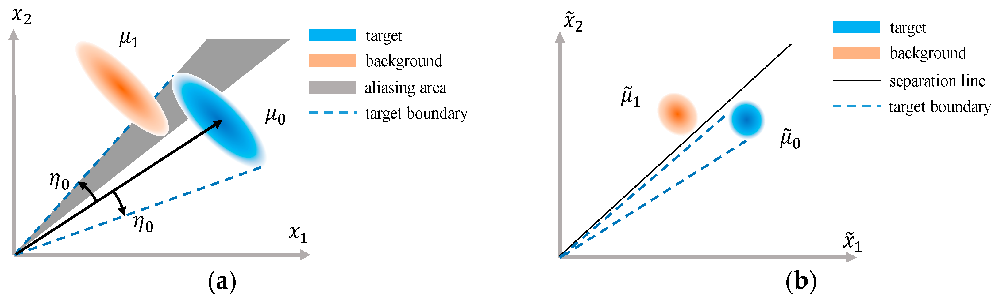
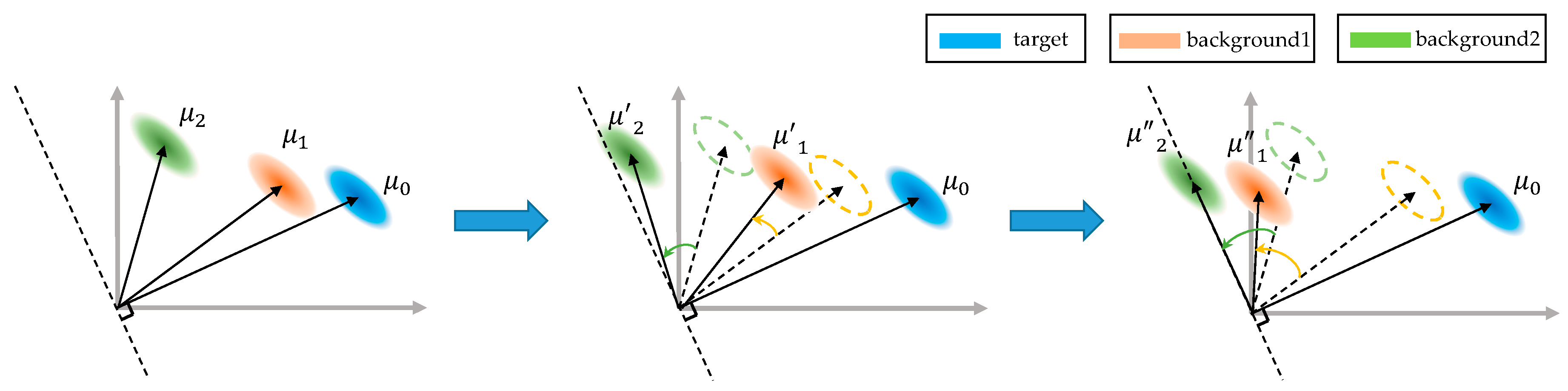
Figure 5 exhibits a simple diagram, where ${\mu }_0$ represents the target, and ${\mu }_1$ and ${\mu }_2$ represent two kinds of backgrounds. The dotted line represents the direction perpendicular to the target. As the iteration proceeds, background vectors gradually move away from the target, and tend to move toward the dotted line. As described above, the moving speed of the background vectors depends on the magnitude of the AD between itself and $\mathbf{d}$. A large AD will make the background vector move faster. Background ${\mu }_2$ is farther from the target than background ${\mu }_1$ in the initial state, so background ${\mu }_2$ will reach the dotted line first. Whether it is fast or slow, the background vectors will eventually move to the dotted line, and in this moment, the target and the background pixels are separated. In the diagram, two types of backgrounds are adopted to illustrate the basic idea. In practice, uninteresting backgrounds usually contain multiple categories, which are often more complex rather than single categories [6,39]. The proposed method could be viewed as follows: Different categories of backgrounds are separated in turn, according to the AD between them and the prior target spectrum, and the target is finally retained.

The AD metric between the background and the target is an important factor for separating the background. In the proposed method, the AD is calculated by the whitened data rather than the original data. If the original data are directly used to calculate the AD between $\mathbf{x}$ and $\mathbf{d}$ to separate background pixels, a serious aliasing phenomenon will still exist. The overlapping part of the target and background pixels is hardly separated, because these pixels in the aliasing area will move uniformly as they have the same AD to the given prior target. As stated in Section 2, the whitening transformation can alleviate the aliasing phenomenon, thus it is appropriate and reasonable to calculate the AD by whitened data rather than original data to separate the background.

As mentioned above, the proposed method employs a hierarchical structure and the AD metric in the whitened space between the spectra of tested pixels and the prior target. In this paper, the lowercase letter k is used to describe the number of layers reached by the current process, that is, the number of iterations. It starts at 1 and adds 1 for each new iteration until the end of the iteration. We use ${\mathbf{x}}_n^k$ and ${\tilde{\mathbf{x}}}_n^k$ to represent the vector of the nth tested pixel in the kth layer before and after the whitening process, respectively. $\mathbf{d}$ is the prior target spectrum, and ${\mathbf{d}}^{\perp }$ is a vector orthogonal to $\mathbf{d}$. ${\mathbf{d}}^{\perp }$ can be generated by solving equation ${\mathbf{d}}^T\mathbf{x}=0$. $\mathbf{d}$ and ${\mathbf{d}}^{\perp }$ are perpendicular to each other, satisfying the equation ${\mathbf{d}}^T·{\mathbf{d}}^{\perp }=0$, so ${\mathbf{d}}^{\perp }$ is one solution of equation ${\mathbf{d}}^T\mathbf{x}=0$. The output of the kth layer is formulated as follows, and it produces the nth tested pixel in the (k + 1)th layer:

$${\mathbf{x}}_n^{k+1}=(1-{\alpha }_n^k){\mathbf{x}}_n^k+{\alpha }_n^k{\mathbf{d}}^{\perp },\hspace{1em}n=1,2,\cdots ,N.$$

(8)

In Equation (8), ${\alpha }_n^k$ is a parameter determining the degree of change in ${\mathbf{x}}_n^k$ and it should be located in [0, 1]. Because the change of ${\mathbf{x}}_n^k$ is related to the AD between ${\tilde{\mathbf{x}}}_n^k$ and ${\tilde{\mathbf{d}}}^k$, the value of parameter ${\alpha }_n^k$ can be obtained through the AD metric, which is denoted as ${\theta }_n^k$. The following equation is the expression of ${\theta }_n^k$:

$${\theta }_n^k=\arccos \left\{\frac{\left|{({\tilde{\mathbf{x}}}_n^k)}^T·{\tilde{\mathbf{d}}}^k\right|}{\Vert {\tilde{\mathbf{x}}}_n^k\Vert ·\Vert {\tilde{\mathbf{d}}}^k\Vert }\right\},\hspace{1em}n=1,2,\cdots ,N,$$

(9)

where ${\tilde{\mathbf{d}}}^k$ is the whitened target spectrum in the kth layer. The absolute value operation is to ensure that the obtained angle is between 0 and 90 degrees. A large ${\theta }_n^k$ makes its corresponding ${\tilde{\mathbf{x}}}_n^k$ change faster, so the size of ${\alpha }_n^k$ should increase with the increase of ${\theta }_n^k$. Here, the power function is adopted to calculate the ${\alpha }_n^k$:

$${\alpha }_n^k={\left[{\theta }_n^k/90\right]}^p.$$

(10)

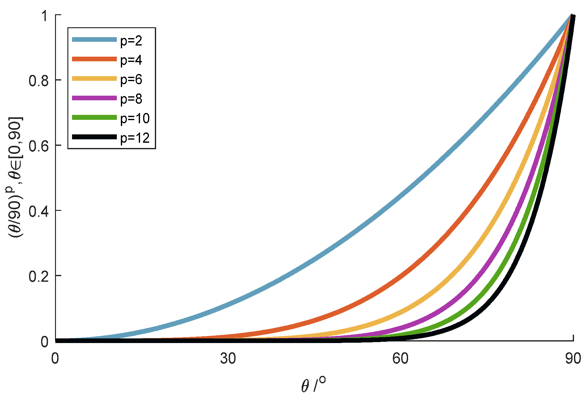
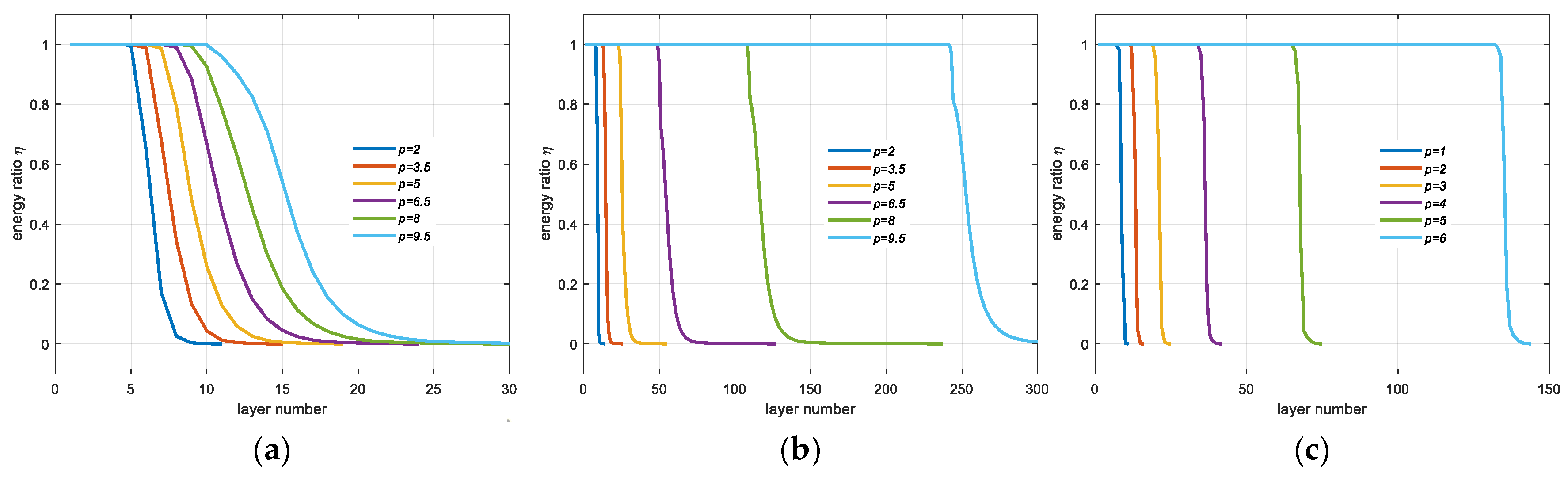
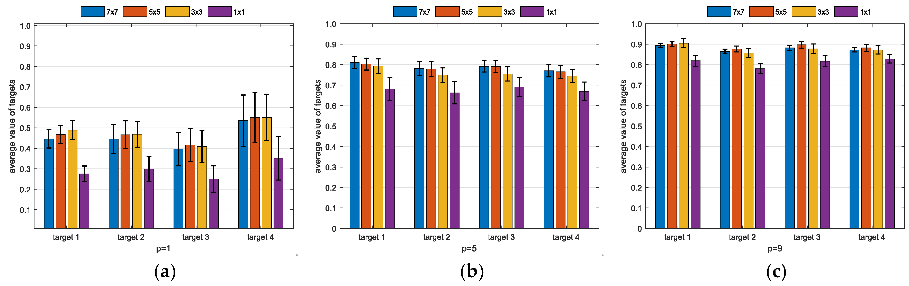
The parameter of the power function p controls the rate of change of ${\alpha }_n^k$, and further controls the moving speed of ${\mathbf{x}}_n^k$ in the direction of ${\mathbf{d}}^{\perp }$. The constant 90 in the denominator ensures that ${\alpha }_n^k$ is between 0 and 1. The effect of parameter p for Equation (10) is shown in Figure 6.

As can be seen from Equation (8), in each layer, part of the tested pixel is replaced by ${\mathbf{d}}^{\perp }$, and thus pixels will gradually transfer to ${\mathbf{d}}^{\perp }$ in the perspective of the AD metric. There are three reasons why we use Equation (8) to adjust the pixel value:

• It can make the backgrounds shift to the direction perpendicular to the target, thus gradually increasing the AD metric between the background and the target pixels.
• It can gradually turn all backgrounds into one genuine category. In HSI target detection, all non-target pixels are considered as background pixels. Some algorithms, such as SMF and ACE, treat the background as one single category. However, there is not only one species of background in real applications, which is an obstacle in the TD problem. Under the adjustment of Equation (8), layer by layer, all background pixels tend to move toward to the same point ${\mathbf{d}}^{\perp }$ and turn to one category, which is helpful for solving the TD problem.
• It can converge the final result. As long as the pixel is not exactly equal to the given target spectral vector, it will eventually be captured by the point ${\mathbf{d}}^{\perp }$ under limited iterations.

As mentioned in third point, if one pixel is not exactly equal to the prior target spectrum, even if it belongs to the target, it will also tend to move toward ${\mathbf{d}}^{\perp }$, finally reaching the point determined by ${\mathbf{d}}^{\perp }$ after sufficient iterations. The different $\theta$ values of the tested pixels make them move away from the given target spectrum at different speeds; consequently, during the continuous iteration process, the AD between the target and background pixels will gradually enlarge at first, and then slowly decrease thereafter. The reason for this decrease is as follows: When the backgrounds have been separated but the iteration process has not stopped, the target pixels, which are not exactly identical to the prior target $\mathbf{d}$, also begin to move in the direction orthogonal to $\mathbf{d}$. Thus, the iteration process should be stopped in an appropriate state, in which the majority of the backgrounds have converged to ${\mathbf{d}}^{\perp }$, and where there exists a large AD between the target and the background pixels.

Assuming that the iteration is stopped after the Kth layer, a new dataset is obtained, represented as ${\mathbf{x}}_n^K,n=1,2,\cdots ,N$. The final detection result is obtained by the AD between the new data ${\mathbf{x}}_n^K$ and the given prior target spectrum $\mathbf{d}$:

$$y_n^K=\arccos \left\{\frac{\left|{({\mathbf{x}}_n^K)}^T·{\mathbf{d}}^K\right|}{\Vert {\mathbf{x}}_n^K\Vert ·\Vert {\mathbf{d}}^K\Vert }\right\}\mathrm{or}{y}_n^K=\frac{{({\mathbf{x}}_n^K)}^T·\mathbf{d}}{\Vert {\mathbf{x}}_n^K\Vert ·\Vert \mathbf{d}\Vert }=\cos ({\theta }_n^K).$$

(11)

These two expressions are equivalent. Thus, we took the second case to analyze the stopping criterion. In fact, each iteration can obtain one detection result. We use ${\mathbf{y}}^k=[y_1^k,\cdots ,y_N^k]$ to represent the detection result of the kth iteration, and employ ${\Vert {\mathbf{y}}^k\Vert }_2^2$ to represent the energy of the result. As the iteration proceeds, the AD between the background and target pixels becomes larger and the cosine value becomes smaller. Thus, the energy of the detection results decreases. According to the trend of the energy decrease, we stopped the iterations by creatively setting a threshold, which was formulated by the following equation. Herein, we used the energy of the first layer detection result as a reference:

$$\eta =\frac{{\Vert {\mathbf{y}}^k\Vert }_2^2}{{\Vert {\mathbf{y}}^1\Vert }_2^2}\underset{\mathrm{stop}}{\overset{\mathrm{continue}}{\gtrless }}{\eta }_0,$$

(12)

where ${\eta }_0$ is a threshold.

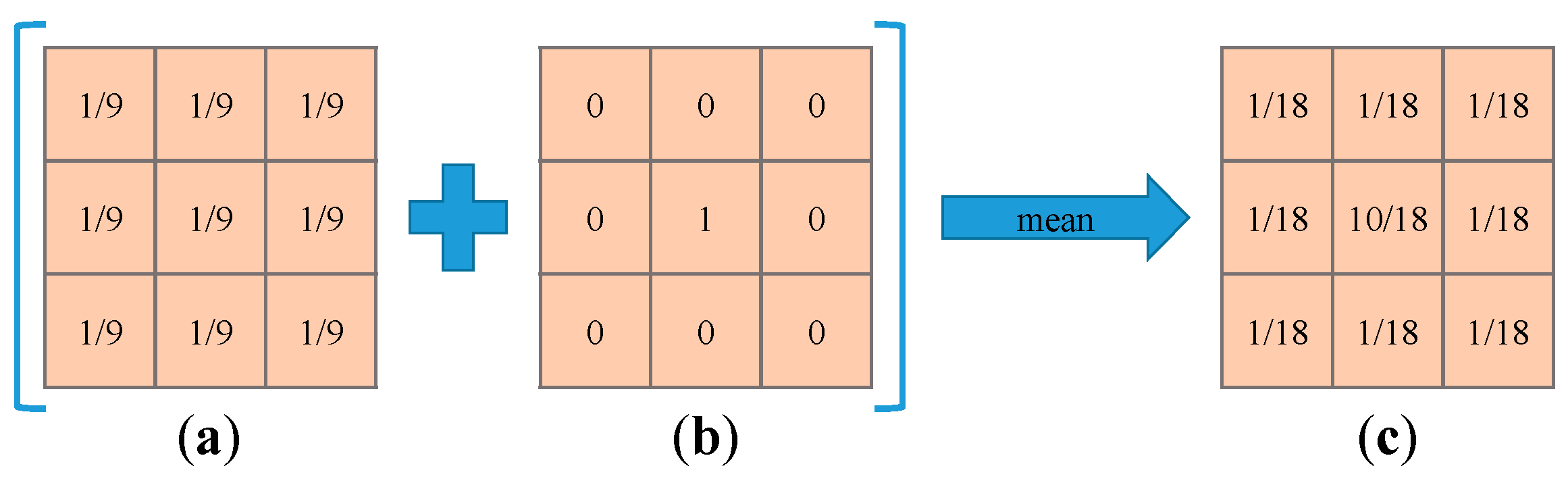
In the first section, we mentioned that a series of interference factors leads to spectral variability, which degrades the accuracy of the TD task. Similarly, the same effect occurs in the AD metric between pixels. Here, a simple smoothing preprocessing operation is adopted, which can be seen as noise reduction, to further improve the detection result. The smoothing preprocessing operation uses a $3\times 3$ mask as shown in Figure 7c. When we directly employed the mask in Figure 7a, the difference between adjacent pixels of the same class was reduced; however, the degree of aliasing between adjacent pixels of different categories increased. Finally, a compromise method was adopted: The mean of the original image and the smoothed image.

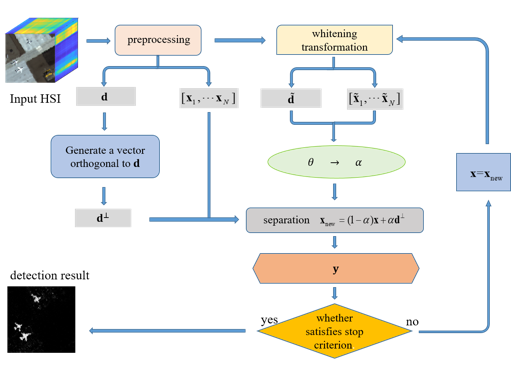
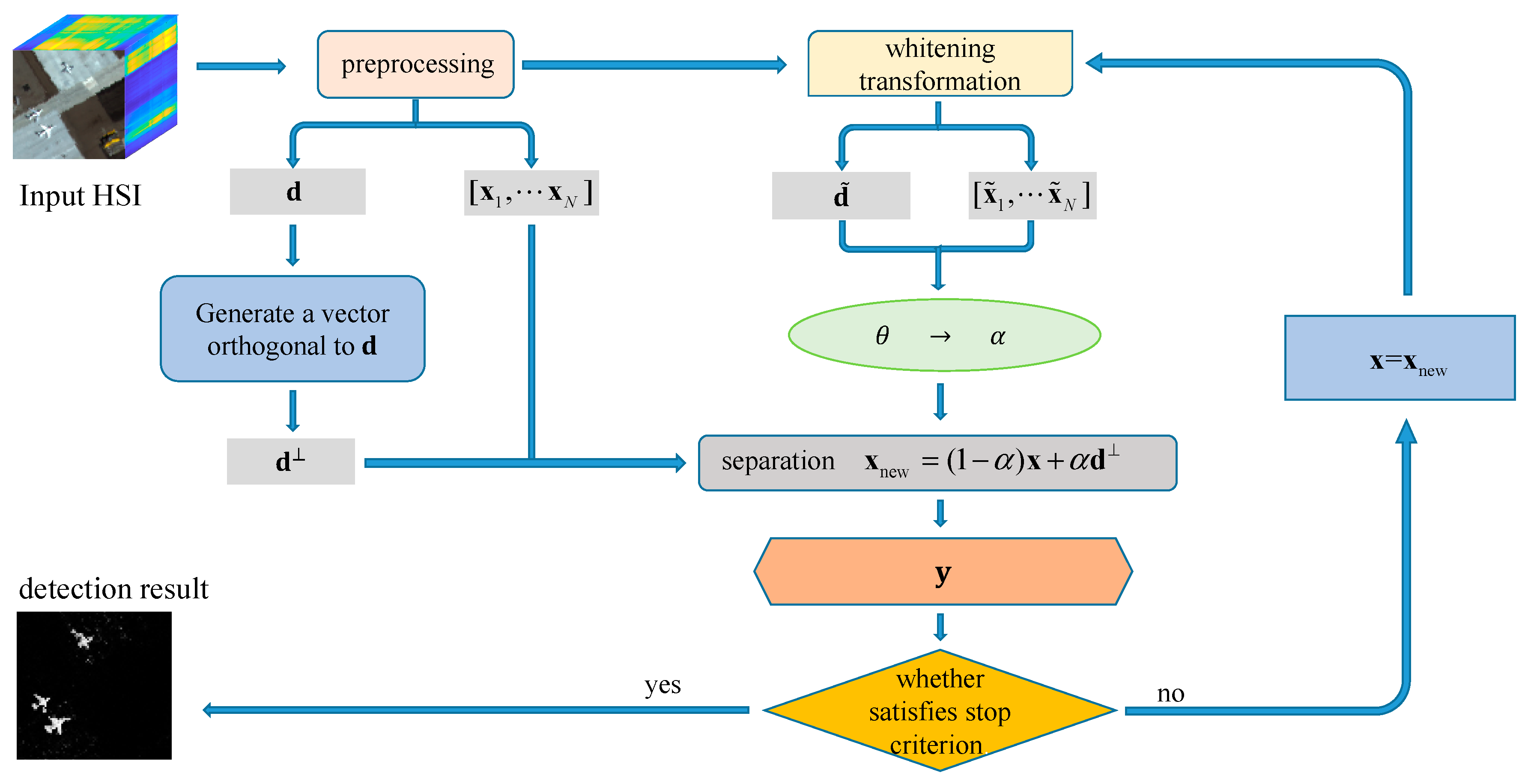
Figure 8 shows the flowchart of the proposed ADHBS algorithm, which includes the following steps:

Step 1:

Smooth the input HSI;

Step 2:

Generate a vector ${\mathbf{d}}^{\perp }$ perpendicular to the target spectral vector $\mathbf{d}$;

Step 3:

Implement the whitening treatment and obtain ${\tilde{\mathbf{x}}}_1,\cdots {\tilde{\mathbf{x}}}_N$ and $\tilde{\mathbf{d}}$;

Step 4:

Calculate the value of $\theta$ and $\alpha$, and implement separation operations to obtain ${\mathbf{x}}_{\mathrm{new}}$;

Step 5:

Calculate the result $\mathbf{y}$. If the stopping condition is satisfied, go to step 6; otherwise, $\mathbf{x}={\mathbf{x}}_{\mathrm{new}}$, go to step 3;

Step 6:

Output the detection result $\mathbf{y}$.

Algorithm1 gives the outline of the proposed method.

4. Experiments

In this section, we implemented the experiments on three HSI datasets to estimate the performance of the proposed ADHBS algorithm. Then, we compared the performance of the ADHBS method with nine competitive methods, including CEM, ACE, SMF, SAM, MSD, CEM-IC, STD, SRBBH, and hCEM. The first five methods are traditional and classical methods, and the last four methods have been proposed recently. All experiments were tested by the MATLAB 2018b software package.

Algorithm 1: ADHBS algorithm for target detection in HSI

Input (and preprocessing):

spectral matrix $\mathbf{x}=[{\mathbf{x}}_1,\cdots {\mathbf{x}}_N]\in {\mathbb{R}}^{B\times N}$, target spectrum $\mathbf{d}\in {\mathbb{R}}^{B\times 1}$, threshold ${\eta }_0>0$,

Initialization:$k=0,{\mathbf{x}}_n^1={\mathbf{x}}_n,$$n=1,2,\cdots ,N$

Hierarchical Separation:

1. $k=k+1$

2. ${\mu }^k=(1/N){\sum }_{n=1}^N{\mathbf{x}}_n^k$

3. ${\mathbf{\Gamma }}^k=(1/N){\sum }_{n=1}^N{[{\mathbf{x}}_n^k-{\mu }^k]}^T[{\mathbf{x}}_n^k-{\mu }^k]$

4. ${\tilde{\mathbf{x}}}_n^k={({\mathbf{\Gamma }}^k)}^{-1/2}·{\mathbf{x}}_n^k,{\tilde{\mathbf{d}}}^k={({\mathbf{\Gamma }}^k)}^{-1/2}·\mathbf{d},$              $n=1,2,\cdots ,N$

5. ${\theta }_n^k=\arccos \left\{\left|{({\tilde{\mathbf{x}}}_n^k)}^T·{\tilde{\mathbf{d}}}^k\right|/\left(\Vert {\tilde{\mathbf{x}}}_n^k\Vert ·\Vert {\tilde{\mathbf{d}}}^k\Vert \right)\right\},$ ${\alpha }_n^k={({\theta }_n^k/90)}^p,$  $n=1,2,\cdots ,N$

6. ${\mathbf{x}}_n^{k+1}=(1-{\alpha }_n^k){\mathbf{x}}_n^k+{\alpha }_n^k{\mathbf{d}}^{\perp },$                  $n=1,2,\cdots ,N$

7. $y_n^k=[{({\mathbf{x}}_n^k)}^T·d]/\left(\Vert {\mathbf{x}}_n^k\Vert ·\Vert \mathbf{d}\Vert \right),$                $n=1,2,\cdots ,N$

8. ${\Vert {\mathbf{y}}^k\Vert }_2^2={\sum }_{n=1}^N{(y_n^k)}^2$

Stop Criterion:

9. $\eta ={\Vert {\mathbf{y}}^k\Vert }_2^2/{\Vert {\mathbf{y}}^1\Vert }_2^2$

if $\eta >{\eta }_0$, go back to step 1; else, go to step 9.

Output:

10. ${\mathbf{y}}^k=[y_1^k,\cdots ,y_N^k]$.

Three evaluation criteria were employed for analysis, including the receiver operating characteristic (ROC) curves, the area under the ROC curves, and the separability maps.

The ROC curve is widely used in the TD field. It describes the relationship between the probability of detection (Pd) and the false alarm rate (FAR). Based on the groundtruth image, Pd and FAR can be obtained by changing to different thresholds on the output of the detection system:

$$Pd=\frac{N_c}{N_t},FAR=\frac{N_f}{N_{total}},$$

(13)

where N_c and N_t are the number of correct detection target pixels and the total true target pixels, respectively. N_f and N_total are the number of false alarm pixels and the total pixels, respectively. If one algorithm obtains a higher Pd than another under the same FAR, we can conclude that the former algorithm is better than the latter. When the ROC curves of these two methods are very close, it shows that the detection results of these two methods are very similar, and thus it is difficult to judge which is better. In this case, the area under the ROC curves (AUC) can be used to compare the performance of different methods. Additionally, in order to further illustrate the performance, the normalized AUC at lower FAR (0.001) was added in this paper. The area below the ROC curve with a false alarm rate between 0 and 0.001 was first calculated and then normalized by dividing by 0.001 to obtain the normalized AUC at lower FAR.

The separability maps describe the distribution of the true target and background pixels on the detection results based on the statistical perspective. They can intuitively reflect the degree of separation between targets and backgrounds by different detectors.

In this paper, we used the “null ()” function in the MATLAB 2018b software package to find a group of bases in the null space of ${\mathbf{d}}^T$, and then linearly combined these bases to form ${\mathbf{d}}^{\perp }$. Here, we made the coefficients of all bases equal to 1 and normalized the result of the linear combination so that the length of ${\mathbf{d}}^{\perp }$ was 1. According to [15,21,23,24,25,37], the parameters of the comparison algorithm were taken as follows: For CEM-IC, the radius parameter was set to 60 without normalizing HSI. For hCEM, the parameter of the exponential function was 20. The sizes of the inner and outer windows for MSD, STD, and SRBBH in the three datasets was 13 and 19, 23 and 31, and 13 and 19, respectively. The number of target dictionaries and the dimension of the target subspace were equal to one tenth of the number of target pixels in the dataset. For the ADHBS method, the parameter values of the power function p will be shown in specific experiments.

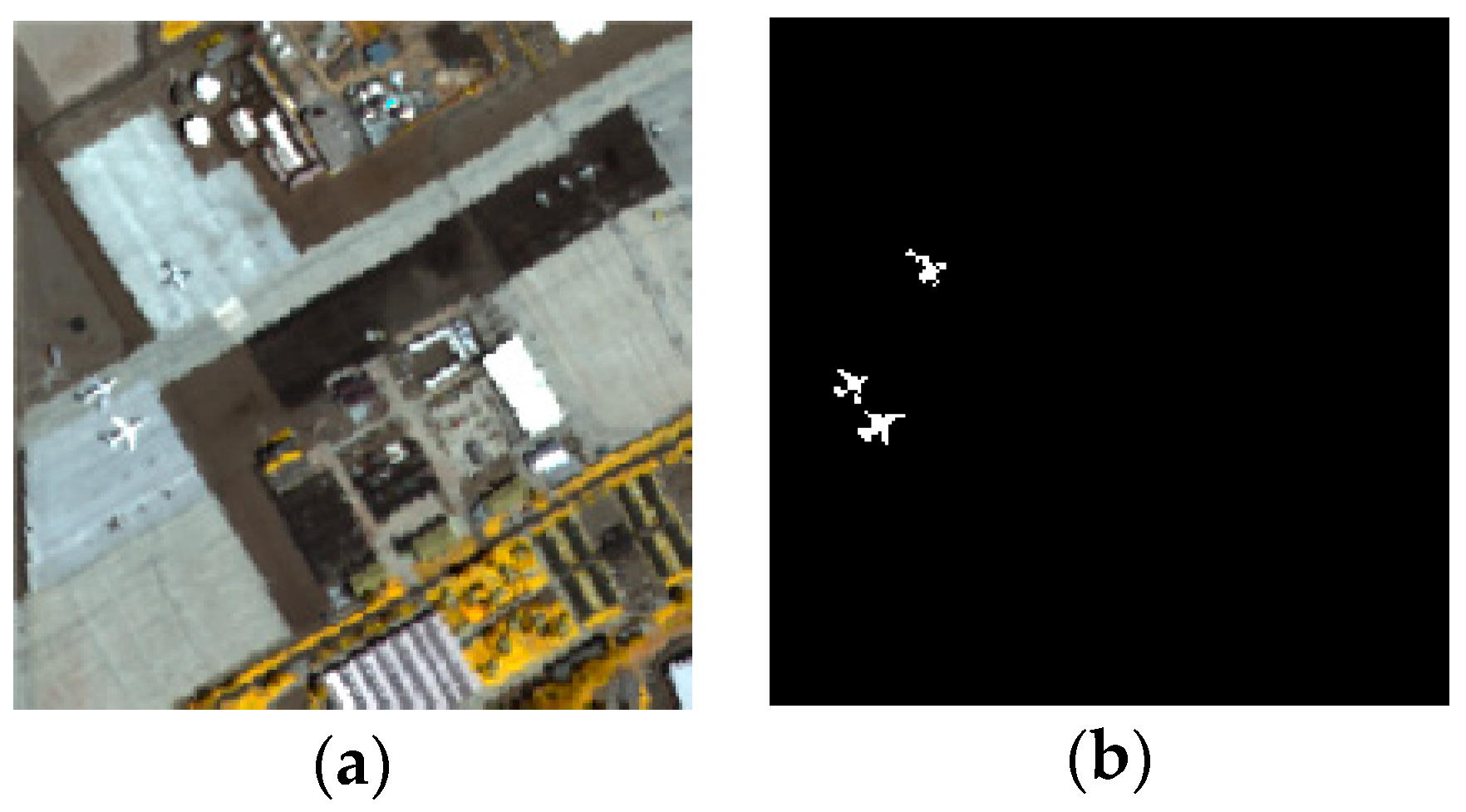
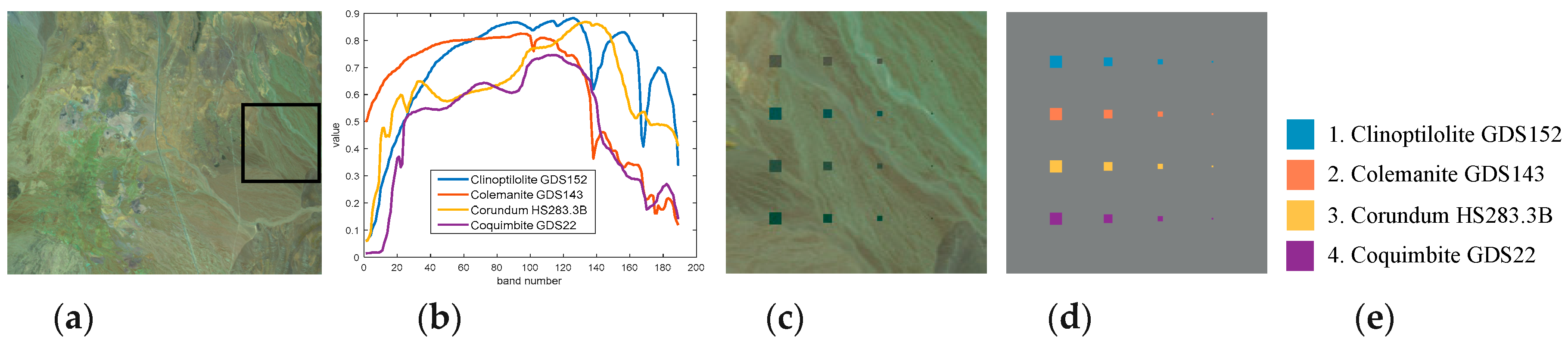
4.1. Experiment on San Diego Airport Data

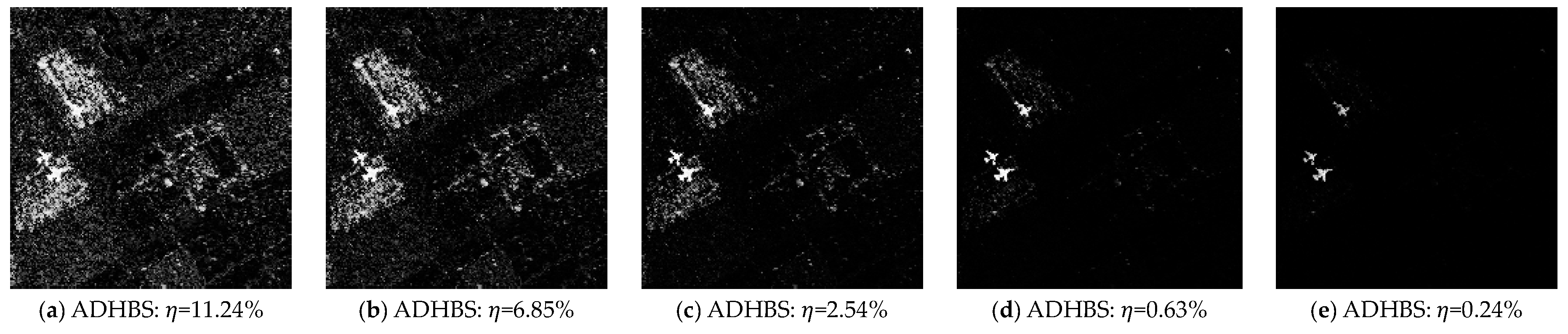
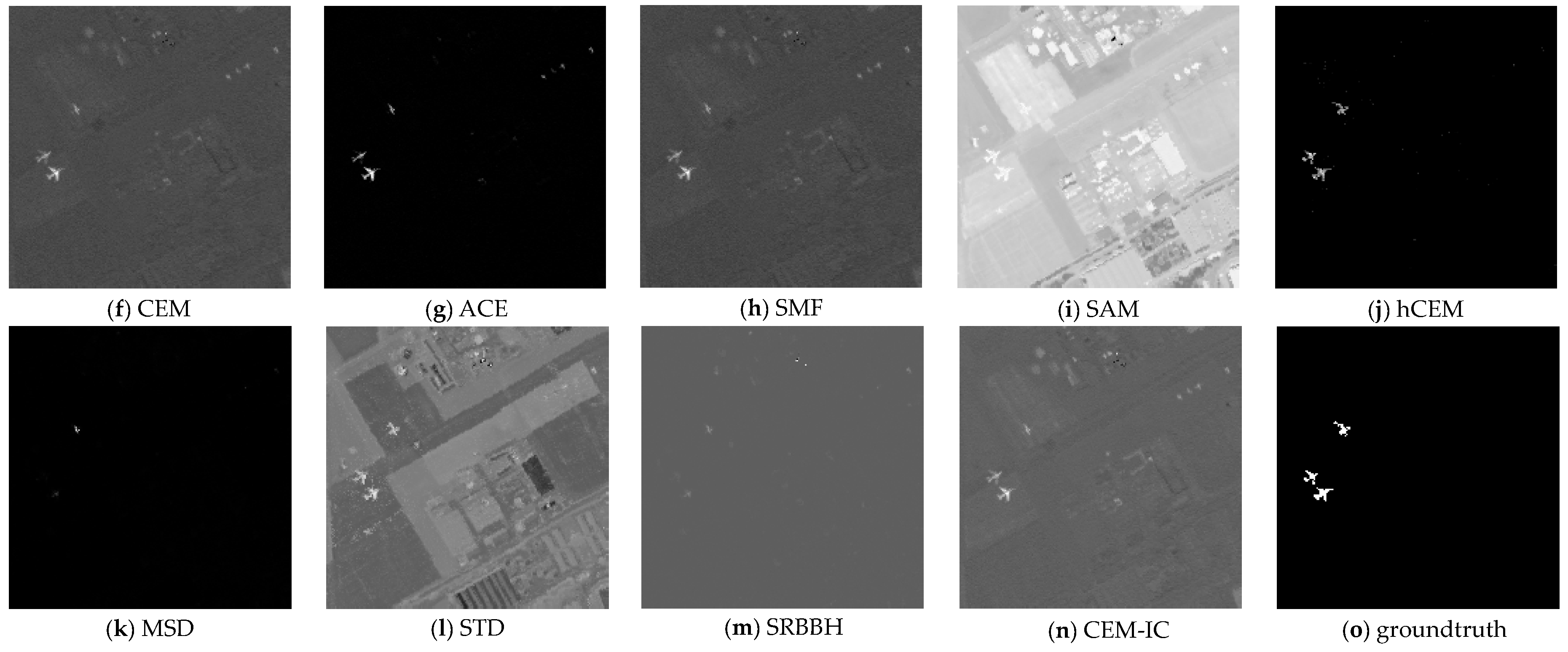
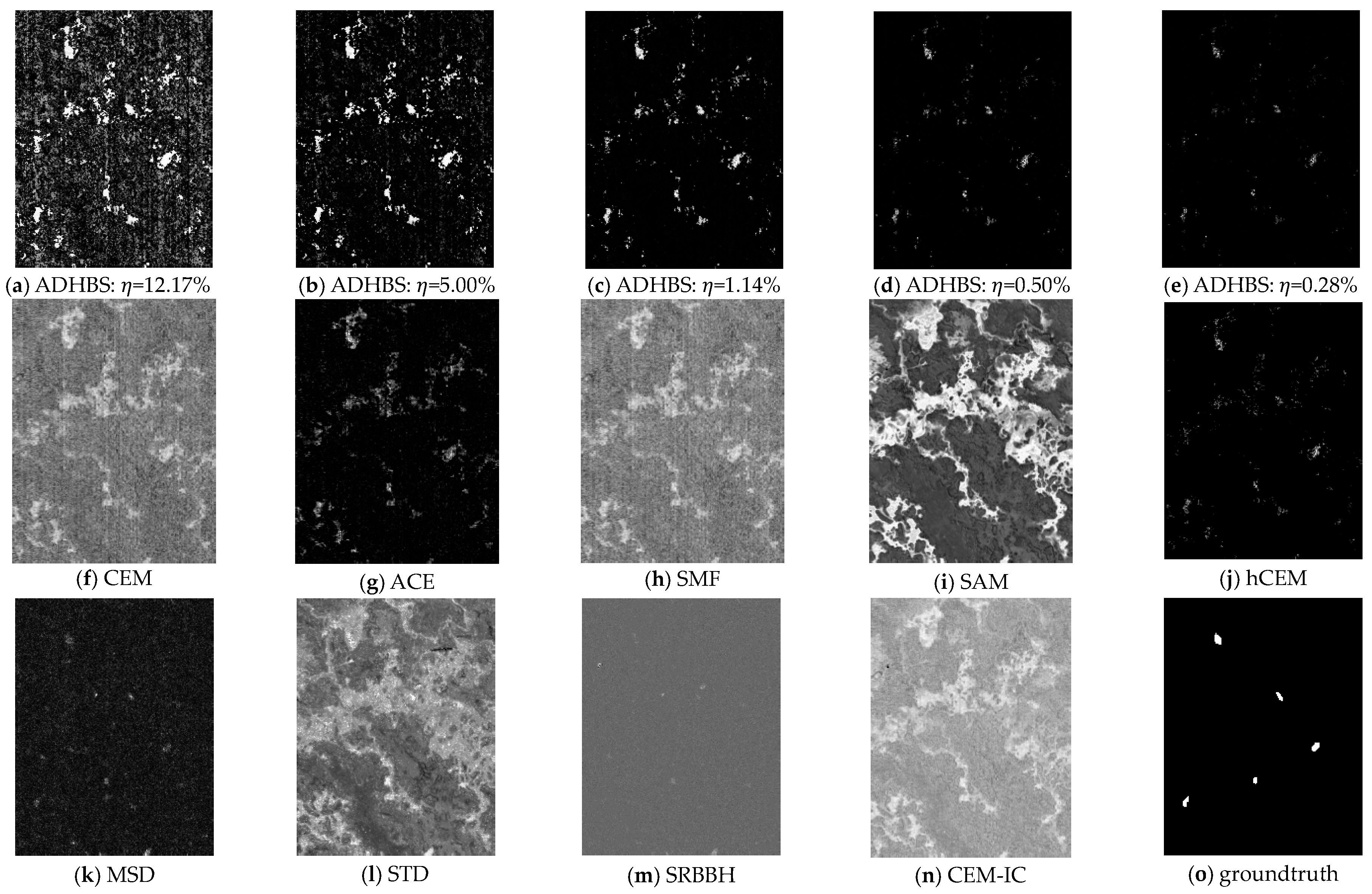
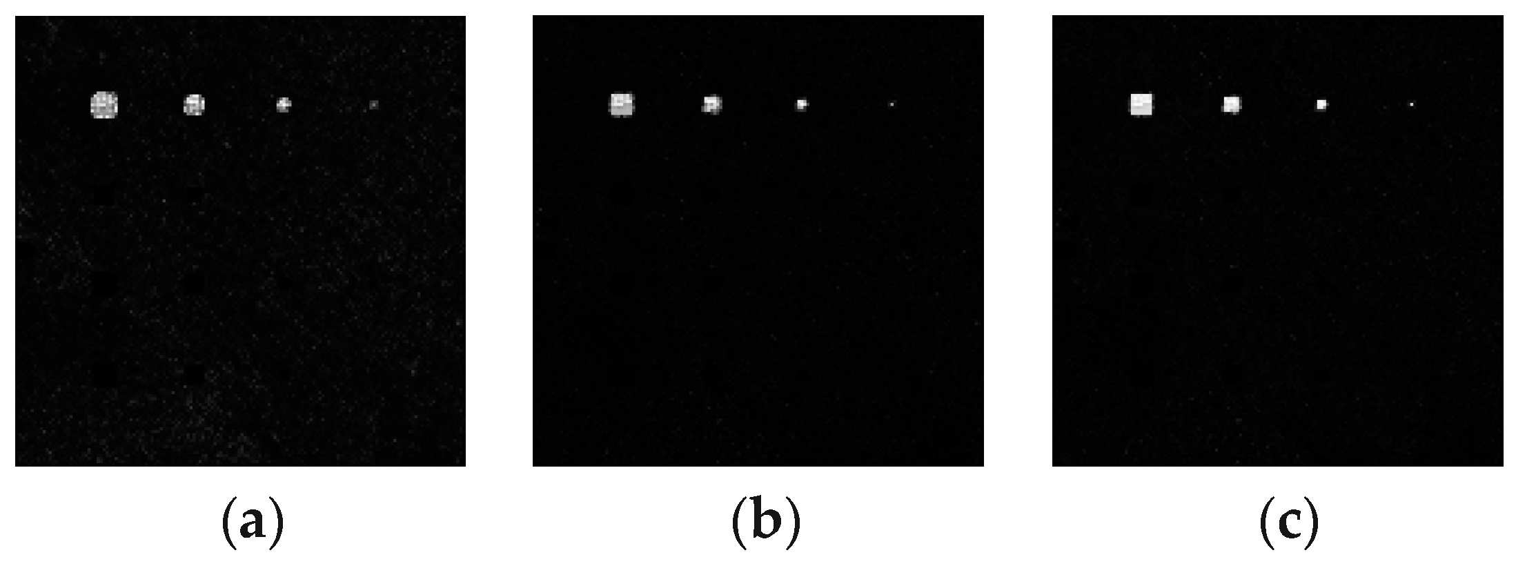
The first HSI dataset was collected by the AVIRIS from the San Diego airport area, which was introduced in Section 2 and shown in Figure 3. This dataset is classical and often appears in the experiments related to HSI target detection. Three airplanes located in the left of the image are targets. The parameter of the power function p takes 8 for the San Diego airport data. The detection results of different methods are shown in Figure 9. According to the variation of $\eta$ in Equation (12) representing the energy ratio of each layer to the initial layer, we exhibit five results corresponding to different $\eta$ in the first row in Figure 9. It can be found that the background pixels are gradually separated as the iteration increases, and the target pixels are retained. The result in Figure 9d is very close to the groundtruth, but there are a few background pixels that have not been separated. The backgrounds in the result of Figure 9e are separated very well. However, the reserved target pixels are not as clear as that in Figure 9d. The result of ADHBS in Figure 9e is similar to the result of hCEM shown in Figure 9j, and their performance is better than the results of the other methods.

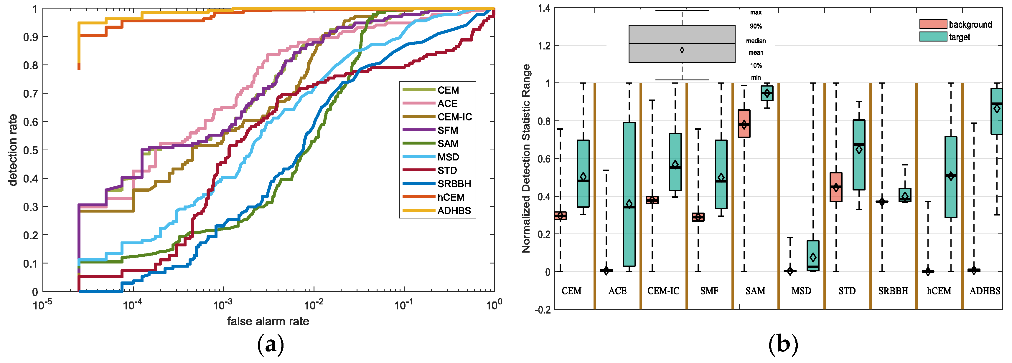
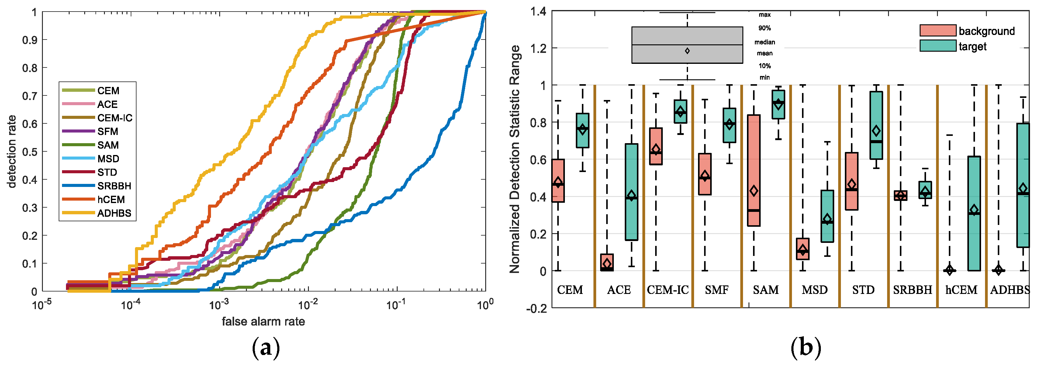
The ROC curves and the separability map for the San Diego airport dataset are shown in Figure 10. The AUC results of the different methods are in the first column of

Table 1. Area under the ROC curves (AUC) value comparison for three datasets (keep four decimal places).

Algorithms	Datasets
	San Diego Airport	Indian Pines	Okavango Delta
CEM	0.9905	0.9985	0.9793
ACE	0.9772	0.9986	0.9780
CEM-IC	0.9941	0.9959	0.9700
SMF	0.9904	0.9985	0.9802
SAM	0.9860	0.9893	0.9431
MSD	0.9688	0.9952	0.9431
STD	0.8881	0.9792	0.9361
SRBBH	0.9231	0.9758	0.6618
hCEM	0.9925	1.0000	0.8906
ADHBS	1.00001	1.0000	0.9868

¹ the bold represents the maximum.

and

Table 2. Normalized AUC value at lower FAR (0.001) comparison for three datasets (keep four decimal places).

Algorithms	Datasets
	San Diego Airport	Indian Pines	Okavango Delta
CEM	0.5004	0.6906	0.0655
ACE	0.5433	0.6906	0.0909
CEM-IC	0.4506	0.3521	0.0461
SMF	0.5033	0.6906	0.0735
SAM	0.1838	0.2299	0.0038
MSD	0.2931	0.4981	0.0805
STD	0.2491	0.1900	0.1276
SRBBH	0.1438	0.0301	0.0057
hCEM	0.9569	1.0000	0.1994
ADHBS	0.98041	1.0000	0.3228

¹ the bold represents the maximum.

. It is necessary to note that the stop criterion in ADHBS is ${\eta }_0=0.005$, and the iteration in ADHBS stops in the 23rd layer. According to the ROC curves in Figure 10a and AUC in Table 1 and Table 2, it can be found that the performance of the proposed method is better than that for the other methods. The performance of hCEM is only just inferior to that of ADHBS. From the separability map in Figure 10b, we find that the separability between the target and background pixels of ADHBS is the greatest in all the results, and hCEM is the second.

4.2. Experiment on Indian Pines Data

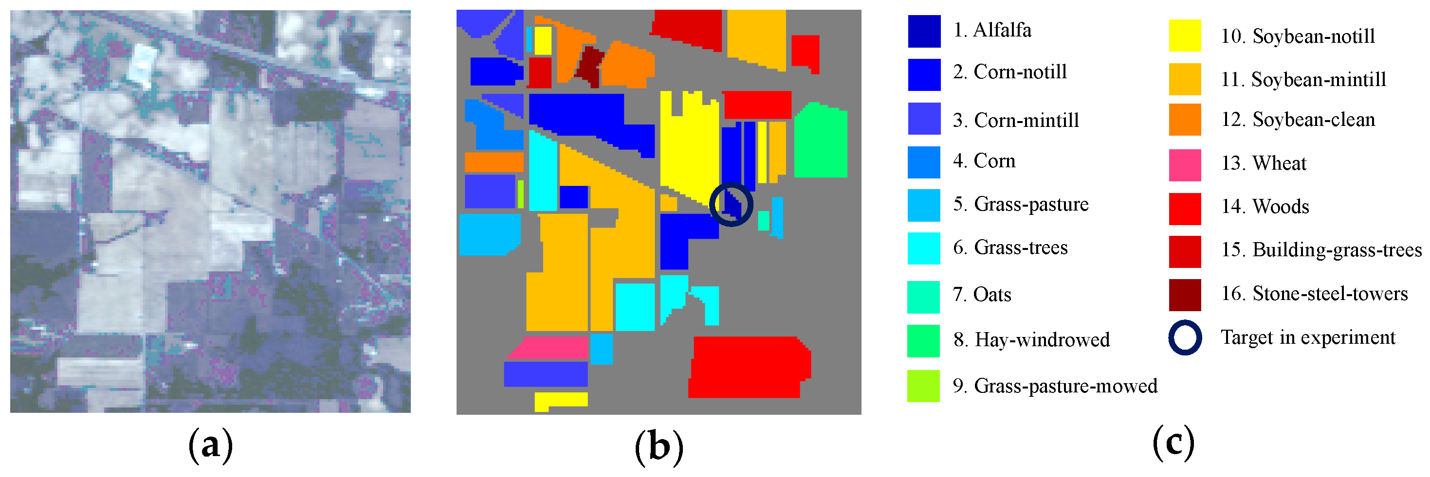
The second HSI dataset was that of Indian Pines collected in North-western Indiana by AVIRIS, which is shown in Figure 11a [40,41]. The image used for the experiment consists of 145 × 145 pixels, which is a subset of a larger scene. This dataset contains 224 spectral reflectance bands covering 0.4–2.5 μm. However, the number of bands is usually reduced to 200 in the case that the bands covering the region of water absorption should be removed. In this data, two-thirds of the area is covered by agricultural vegetation, and the remaining one-third is covered by forest or other natural perennial vegetation. The dataset includes 16 kinds of marked vegetation, such as alfalfa, oats, wheat, etc. Figure 11b,c show the groundtruth and legend of different categories. In our experiment, we chose alfalfa, which accounts for only 0.2% with 46 pixels of this dataset, as the target to test the efficiency of the proposed method. The parameter of power function p takes 6 for this data.

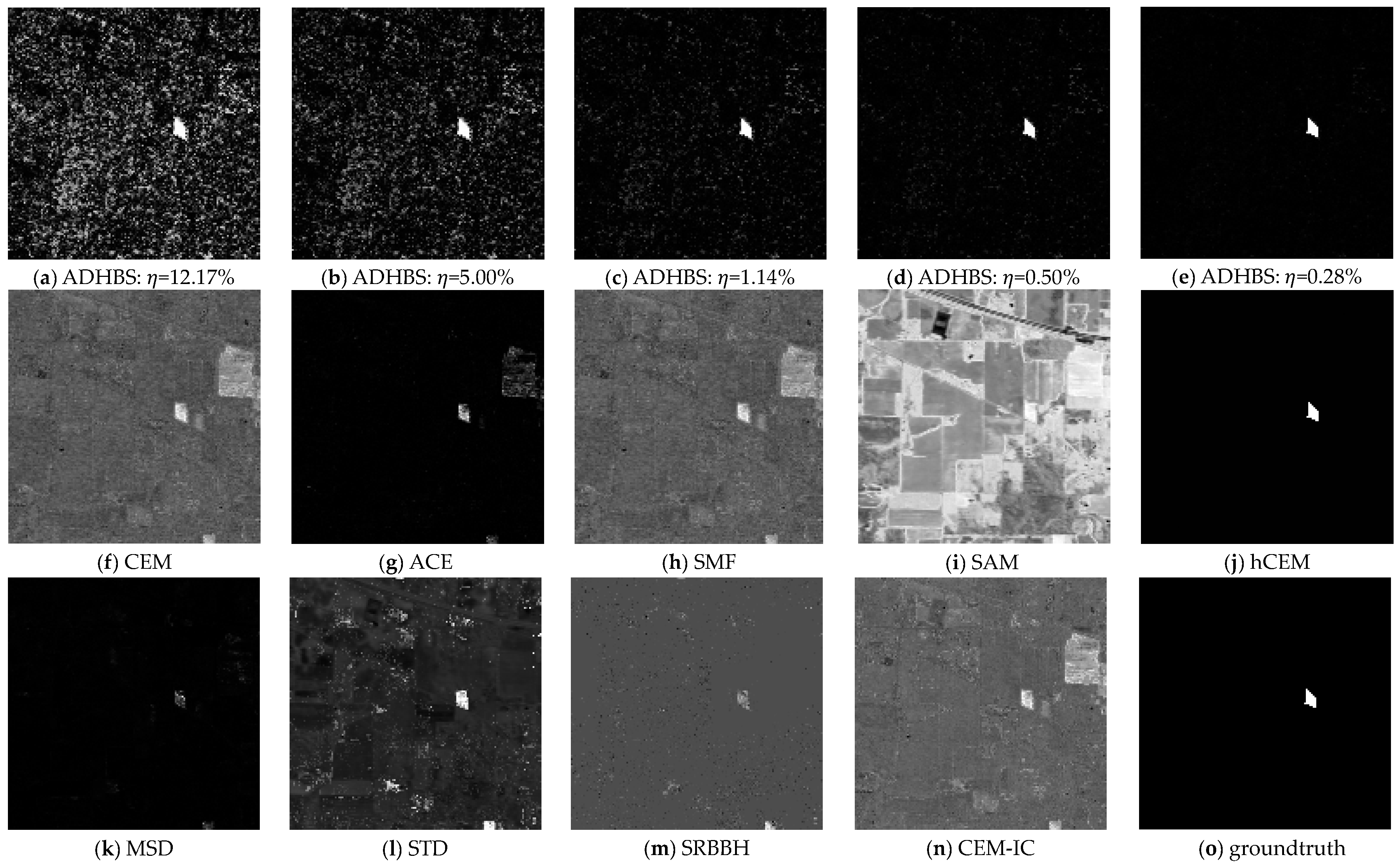
The TD results are shown in Figure 12. The ground truth of the target is shown in the last sub-image. Five results from different layers in ADHBS are exhibited in the first row of Figure 12. They correspond to different $\eta$ values. The background pixels gradually separate and the target pixels are retained. For this data, the results of ADHBS and hCEM shown in Figure 12e,j are both accurate. Other methods result in either incomplete background separation or the target being suppressed, resulting in poor detection performance.

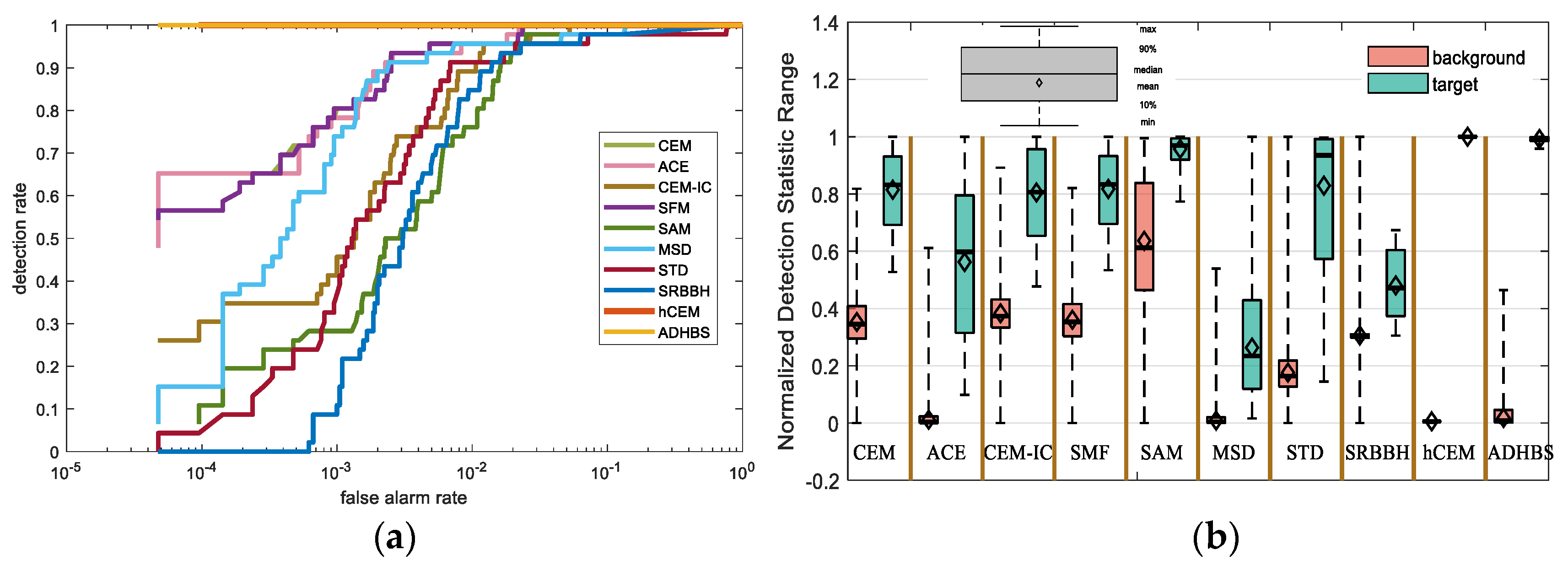
The iteration in ADHBS stops in the 58th layers for this data when the stop criterion is set to ${\eta }_0=0.005$. The output is used for calculating the evaluation criterion. The ROC curves and the separability map for the Indian Pines data are shown in Figure 13. The AUC results of the different methods are in the second column of Table 1 and Table 2. In Figure 13a, the curves of ADHBS and hCEM coincide, so we increased the width of the curve corresponding to hCEM for more convenient observation. Obviously, the performances of ADHBS and hCEM are the best. In the separability map, hCEM perfectly separates the target from the backgrounds, and the separation performance of ADHBS is second only to hCEM.

4.3. Experiment on Okavango Delta Data

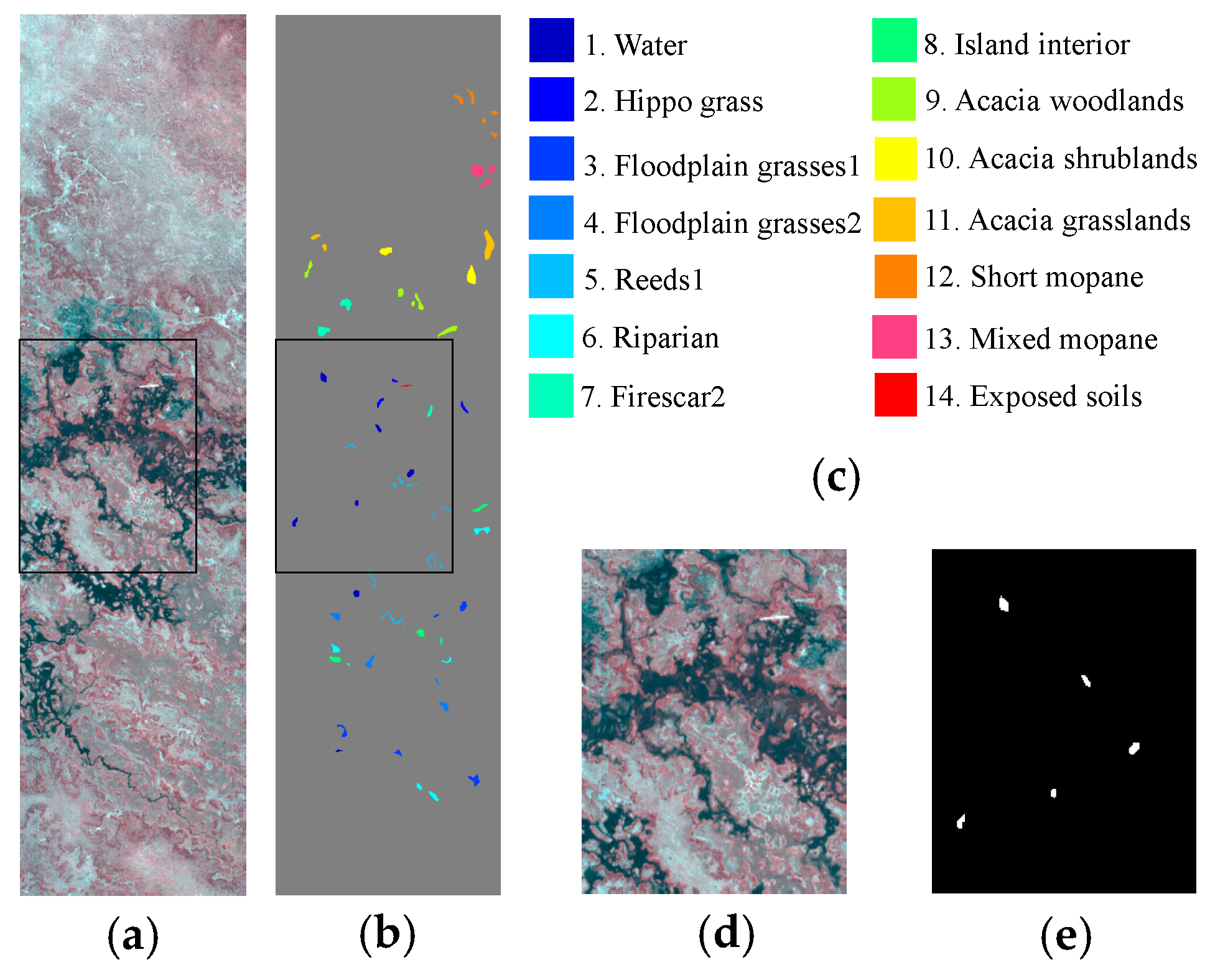
The third tested dataset was acquired from the Okavango Delta, Botswana in 2001–2004 by the National Aeronautics and Space Administration (NASA) EO-1 satellite [42]. It includes 242 bands covering a 400- to 2500-nm portion of the spectrum in 10-nm windows. After removing the low SNR and bad bands, 145 bands were retained. This dataset consists of 14 identified classes representing different land covering types in seasonal swamps, occasional swamps, and drier woodlands located in the distal portion of the Okavango Delta. Specific categories are water, riparian, grasslands, etc. The sense of this Okavango Delta data is shown in Figure 14a, consisting of $1000\times 256$ pixels. Figure 14b,c show the ground truth and legend of different categories. Here, we chose the area covered by water as the target. A subset of this data enclosed by a black box was chosen to implement the experiment. In order to show clearly the distribution state of the target, the subset with the corresponding ground truth of water is shown in Figure 14d,e. The size of the subset is $260\times 200$. The parameter of power function p takes 6 for the Okavango Delta data. The detection results are shown in Figure 15. As in the previous two experiments, the first row of Figure 15 is used to show the results of the proposed method from different layers corresponding to different values of $\eta$. In the iteration process, the background pixels of the image are gradually separated. The target pixels in Figure 15a–c are detected well by ADHBS, but there are still a lot of unseparated background pixels around the target and other areas. In Figure 15d,e, the residual state of the background pixels is improved. Meanwhile, the interesting target pixels are also suppressed to some extent but without affecting discrimination. ACE and hCEM are inferior to ADHBS in the separation of target and background pixels but better than the other methods. The target pixels in the output of the other methods are submerged in the undivided backgrounds.

For this data, the iteration in ADHBS stops in the 141st layer when the stop criterion is ${\eta }_0=0.005$. The ROC curves and the separability map are exhibited in Figure 16. Furthermore, the AUC results are listed in the third column of Table 1 and Table 2. From the ROC in Figure 16a and AUC in Table 1 and Table 2, we find that the performance of ADHBS is the best. In the separability map, it is easily seen that the ACE, hCEM, and ADHBS can suppress most of the background very well, but for the hCEM method, it suppresses the target more than the other two methods. That is why the AUC value of hCEM is lower than that of ACE and ADHBS.

Through the above three groups of experiments, we can draw the conclusion that the proposed method has better ability to separate background pixels and retain target pixels than the other methods. At the same time, we find that hCEM also shows good detection results. It should be noted that both hCEM and ADHBS adopt hierarchical structures. In other words, both of them use the prior target information more than once. The experimental results show that better detection results can be obtained by fully utilizing the target information.

5. Discussion

5.1. The Effect of Parameter

In the proposed method, parameter p and parameter ${\eta }_0$ play a crucial role. The size of parameter p determines the value of parameter α, which affects the accuracy and the speed of background separation. The size of parameter ${\eta }_0$ controls the stop condition. Both of them decide the size of the hierarchical structure and the quality of the detection results. In this section, the effect of p and ${\eta }_0$ were analyzed by choosing different values to implement experiments.

The variation range of parameter p is between 1 and 10, with intervals of 0.5. The speed of background separation controlled by p can be reflected by the $\eta$ value in each layer. The separation of background pixels leads to a decrease of energy in the detection result, and further causes $\eta$ to become smaller. Figure 17 shows the change of $\eta$ values following iteration under different p values for the three datasets. Only part of the p values’ test results are displayed for convenient observation, but without impacting the analysis. Based on Figure 17, it can be found that the smaller the p value, the faster the $\eta$ value decreases. This means that the faster the background separation, the faster the algorithm can stop, which is consistent with the illustration in Section 3. The reason for this is as follows: In the case of the same θ value in Equation (10), the smaller value of p makes the α become larger. Parameter α controls the step size of the background pixels away from the given target spectrum, so a large α results in a faster speed in background separation. It is necessary to note that a fast algorithm convergence does not mean good detection results, which will be discussed later.

Table 3. The number of iteration layers under different p values for the three datasets.

Data	p Values
	1	1.5	2	2.5	3	3.5	4	4.5	5	5.5	6	6.5	7	7.5	8	8.5	9	9.5	10
1st 1	7	8	9	10	11	12	13	15	16	17	18	19	20	21	23	24	26	27	30
2nd 2	8	10	11	13	16	19	23	30	36	46	58	76	89	115	149	190	233	307	411
3rd 3	10	13	15	19	24	30	40	53	72	100	141	202	292	428	632	939	1404	2103	3170

¹ San Diego airport dataset; ² Indian Pines dataset; ³ Okavango Delta dataset.

gives the number of iteration layers under different p values when the stopping criterion is ${\eta }_0=0.005$.

The standard AUC was used to evaluate the performance of the detection results. Meanwhile, we also considered the influence of different stopping criterion on the final detection results. Here, we chose 15 different values of stopping criterion ${\eta }_0$, and they were obtained by multiplying 9, 7, 5, 3, and 1 by ${10}^{-2}$, ${10}^{-3}$, and ${10}^{-4}$, respectively. Figure 18 shows the standard AUC of the detection results under different p and ${\eta }_0$ values for the three datasets. The performance of the second dataset is relatively stable, only fluctuating at one point. For the San Diego airport data, when the p value is small or the ${\eta }_0$ value is large, the test result is not good. When the background pixels are away from the target and move toward the direction perpendicular to the target spectrum, the small p value causes the background pixels to adjust too much, which makes them skip the best point and produce deviation. The lack of accuracy leads to inaccurate separation of the background and target pixels, which affects the accuracy of the detection results. Large ${\eta }_0$ values cause the algorithm to stop prematurely, so that the background pixels are not completely separated, as well as further reduce the quality of the detection results. For the third dataset, when the p value is smaller than 5, the performance of the results fluctuates greatly. When the p value is larger than 5, the rule of the detection results is basically consistent with the first dataset: The test result is not good when the p value is small or the ${\eta }_0$ value is large. If we look closely at Figure 18a,c, it can be found that under a fixed p value, such as 8 or 6, the AUC increases first and then decreases slightly thereafter. Combining the experimental results of Section 4, especially from the first and third experiments, we make the following analysis: Smaller stopping criterion will result in some target pixels becoming unclear in the results, such as the results in Figure 9e and Figure 17e. The experiments show that the choice of ${\eta }_0$ value can be between 0.001 and 0.01. A larger p value can be selected to achieve better results. However, it is worth noting that when the p value is large enough, an increase of the p value has little effect on the final result, which can also be seen from Figure 18.

5.2. The Effect of Target Size

In this section, one synthetic datum is adopted to analyze the performance of the proposed method for different sizes of targets. The Cuprite dataset shown in Figure 19a was collected by AVIRIS. A region with the size of 150 × 150 pixels enclosed by a black box was selected as the background of the synthetic data. Four spectra from the U.S. Geological Survey (USGS) were employed as the target spectra and are shown in Figure 19b, including Clinoptilolite GDS152, Colemanite GDS143, etc. The Cuprite dataset contains 224 bands and retains 189 bands after the removal of low-SNR and water absorption bands. Each spectrum in Figure 19b was used to construct four targets with different sizes of 7 × 7, 5 × 5, 3 × 3, and 1 × 1. These targets were implanted in the background image by replacing their corresponding background pixels, and then were corrupted by a Gaussian white noise with 30-dB SNR. Figure 19c shows the synthetic data, and the corresponding groundtruth is shown in Figure 19d.

Figure 20 exhibits the detection results of the first target category with three different p values. The stopping criterion is ${\eta }_0=0.005$. When the p value is small, the detection result is rough. The three larger targets can be detected; however, a target of size 1 × 1 is almost invisible in Figure 20a. With an increase in p, the targets in the results gradually become visible clearly, as does the other three target categories with different sizes.

The average values of the target pixels in the results were used to further analyze the effect of the target size on the detection performance. They were obtained by averaging the pixel values of one target in the detection results. A target with a large average value in the result means that it is clearer in the detection result, while a target with a small average value is fuzzier in the detection result and is more likely to be missed. The average value of the target reflects the difficulty of detection. We ran 50 experiments under each different p value, and Figure 21 shows the average values of the targets in the detection results.

According to Figure 21, we found that the average values of the targets increase when the p value becomes larger. It means that a large p value is good for detection, which is the same as the conclusion of the last discussion. In order to alleviate the influence of the interference factors that cause the spectral variability, the proposed method adopts one simple smoothing preprocessing operation. Although the target information of the tiny target is lost more than that of a large target caused by the smoothing operation, the target information retained in the tiny target is still much more than that of the background. One small p results in large α, then causes a large step size of the tested spectrum away from the given target spectrum. A large step size not only accelerates the speed of the spectrum away from the target but also roughs the separation degree of the target and the background. On the contrary, one large p produces a small α and leads to a small step size. A small step size makes the spectrum more precise as it moves, thus increasing the separability between the target and the background, which is better for detecting tiny targets. However, tiny targets lose more target information after all, so in the detection process, the moving distance corresponding to the tiny targets is larger than that of large targets. Therefore, large targets are clearer than tiny targets in the detection results, that is, the average value of the former is larger than that of the latter. In general, the increase of p improves the robustness to the target scale.

5.3. Time Consumed by Algorithms

We compared the time consumption of different TD methods, as shown in

Table 4. Time consumed for the different methods of the three datasets (keep four decimal places, specified in seconds).

Algorithms	Datasets
	San Diego Airport $(200\times 200\times 189)$	Indian Pines $(145\times 145\times 200)$	Okavango Delta $(260\times 200\times 145)$
CEM	0.0290	0.0155	0.0191
ACE	0.1425	0.0836	0.1461
CEM-IC	0.2077	0.3201	0.1150
SMF	0.0897	0.0537	0.0882
SAM	0.0625	0.0344	0.0641
MSD	226.5688	130.2955	241.8973
STD	92.0350	33.2296	187.8326
SRBBH	142.7876	39.7361	341.4231
hCEM	0.5014(15) 1	0.2255(9)	0.3751(12)
ADHBS	3.2665(23)	4.9614(58)	18.6921(141)

¹ the numbers in parentheses represents the number of iterations or layers of the corresponding algorithm.

. The sizes of the corresponding datasets are represented by the numbers below the dataset name. In the last two lines, the number of iterations or layers of the corresponding algorithm is shown by the numbers in parentheses. We used the MATLAB 2018b software to test all the aforementioned methods on an Intel i7 personal computer with 8 GB RAM and 2.20GHz frequency.

CEM, SMF, and SAM are classical single-layer algorithms, thus they consume little time. Although the ACE method is a single-layer algorithm, it involves a whitening process, which contains the square root operation of the matrix. Thus, the relative time consumption is larger than the first three methods. MSD needs to construct the target and background subspace, which uses singular value decomposition for each pixel. Thus, this method consumes time expensively. STD and SRBBH are methods based on sparse dictionary representation. They need to construct a target and background dictionary for each pixel, and adopt the orthogonal matching pursuit (OMP) algorithm to solve the optimization problem, which also needs a lot of time. CEM-IC and hCEM have been proposed in recent years and perform more efficiently. For the proposed method, it adopts a hierarchical structure, the same as hCEM, but the computational complexity is bigger than the latter. This is caused by the existence of a whitening process in each iteration, as well as more iterations for the proposed method.

Furthermore, we briefly discuss the complexity of the proposed method. N and B are used to represent the number of total pixels and the number of bands in HSI, respectively. In the whitening process, the computational complexity (CC) of the calculation about the covariance matrix is O(NB²), and both the matrix inversion and the matrix square root have a CC of O(B³). The CC of the matrix and N vector multiplication is O(NB²). For the adjustment of spectral vectors, the corresponding CC is O(NB²). Therefore, the proposed method’s CC is O(k(N + B) B²), where k represents the total number of iterations.

6. Conclusions

In this paper, we proposed a TD method based on the AD metric with a hierarchical structure. The background pixels are separated according to the AD metric between the prior target and the background pixels in the whitened space, because whitening can alleviate the aliasing phenomenon. In the iteration process of the hierarchical structure, the background pixels are separated in the direction orthogonal to the prior target spectrum. When the iteration stops, there is a clear distinction between the target and the background pixels. A simple smoothing preprocessing operation is employed to alleviate the influence of interference. The experimental results using three real datasets showed that the proposed ADHBS method is superior to the traditional methods, such as CEM, ACE, and SMF, and other recently proposed methods, for instance CEM-IC, STD, and hCEM.

The proposed method employs a hierarchical architecture. It uses more time to obtain the results than classical methods because of the existing iterative process. Therefore, the way in which to reduce the number of iterations is the main contents of future work.