Abstract
Given the impact of tropical forest disturbances on atmospheric carbon emissions, biodiversity, and ecosystem productivity, accurate long-term reporting of Land-Use and Land-Cover (LULC) change in the pre-satellite era (<1972) is an imperative. Here, we used a combination of historical (1958) aerial photography and contemporary remote sensing data to map long-term changes in the extent and structure of the tropical forest surrounding Yangambi (DR Congo) in the central Congo Basin. Our study leveraged structure-from-motion and a convolutional neural network-based LULC classifier, using synthetic landscape-based image augmentation to map historical forest cover across a large orthomosaic (~93,431 ha) geo-referenced to ~4.7 ± 4.3 m at submeter resolution. A comparison with contemporary LULC data showed a shift from previously highly regular industrial deforestation of large areas to discrete smallholder farming clearing, increasing landscape fragmentation and providing opportunties for substantial forest regrowth. We estimated aboveground carbon gains through reforestation to range from 811 to 1592 Gg C, partially offsetting historical deforestation (2416 Gg C), in our study area. Efforts to quantify long-term canopy texture changes and their link to aboveground carbon had limited to no success. Our analysis provides methods and insights into key spatial and temporal patterns of deforestation and reforestation at a multi-decadal scale, providing a historical context for past and ongoing forest research in the area.
1. Introduction
Tropical ecosystem services are severely impacted by deforestation and forest degradation [1,2,3]. Not only does tropical forest Land-Use and Land-Cover Change (LULCC) constitute 10% to 15% of the total global carbon emissions [4] it also changes forest fragmentation and influences forest structure and function [5,6,7]. Strong fragmentation effects decrease the number of large trees along forest edges [8,9], while species composition and biodiversity are equally negatively affected [10,11,12]. Estimates show that 31% of carbon emissions are caused by edge effects alone [6].
Accurate estimates of LULCC and forest canopy structure are therefore imperative to estimate carbon emissions and other ecosystem services [1,2]. Remote sensing products have been key inputs in LULCC assessments as they provide accurate spatial information to help estimate carbon emissions [1,13]. More so, high-resolution aerial images provide scientists with tools to monitor forest extent, structure, and carbon emissions as canopy texture is linked to aboveground biomass [14,15,16]. However, most of these estimates are limited in time to recent decades [1,2,17,18].
Historical estimates of Land-Use and Land-Cover (LULC) in the pre-satellite era (<1972) exist but generally rely on nonspatially explicit data (i.e., socioeconomic data) [2,17,19,20]. Efforts have been made to use other geospatial data sources such as historical maps [21], declassified CORONA satellite surveillance data across the US and central Brazil [22], as well as aerial surveys in post World War II Germany [23]. Survey data across the African continent is less common, inaccessible, or both. Some studies do exist; Buitenwerf et al. [24] and Hudak and Wessman [25] used aerial survey images to map vegetation changes in South African savannas whilst Frankl et al. [26] and Nyssen et al. [27] mapped the Ethiopian highlands of the 1930s.
Across the central Congo Basin, most of these historical images were collected within the context of national cartographic efforts by the “Institut Géographique du Congo Belge” in Kinshasa (then Léopoldville), DR Congo. Despite the existence of large archives of aerial survey imagery of African rainforest (Figure 1, Appendix A Figure A3), as of yet, no studies have valorized these data. The lack of a consistent valorization effort is unfortunate as the African rainforest is the second largest on Earth and covers ~630 million ha, representing up to 66 Pg of carbon storage [28] and currently loses forest at an increasing pace [29]. Given the impact of LULCC on the structure and functioning of central African tropical forests and their influence on both carbon dynamics [30] and biodiversity [12], accurate long-term reporting of historical forest cover warrants more attention [21].
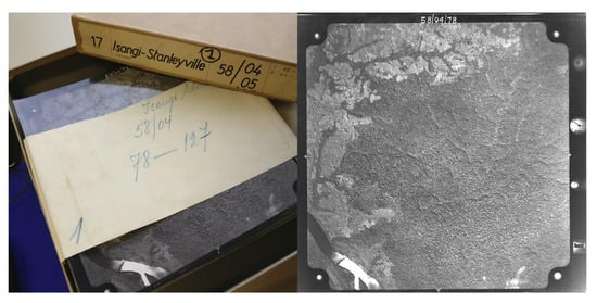
Figure 1.
A box of historical aerial photographs (left) and a single aerial photograph (right) showing part of the Congo river: Note the metadata provided in the right side margin of the image, such as acquisition time and flight height.
Here, we use a combination of historical aerial photography (1958) and contemporary remote sensing data (2000–2018) to map long-term changes in the extent and structure of the tropical forest surrounding Yangambi (DR Congo) in the central Congo Basin, effectively linking the start of the anthrophocene [31] with current assessments. Yangambi was, and remains, a focal center of forest and agricultural research and development in the central Congo Basin. Past research in the region allows for thorough assessment of LULCC from a multidisciplinary point of view, confronting us with complex deforestation and land-use patterns.
We leverage structure-from-motion to generate a large orthomosaic of historical imagery and to develop a convolutional neural network-based forest cover mapping approach based upon a semi-supervised generated dataset extensively leveraging data augmentation. Our methodology aims to provide a historical insight into important LULCC spatial patterns in Yangambi, such as fragmentation and edge complexity. We further contextualize the influence of changes in the forest’s life history on past and current research into Aboveground Carbon (AGC) storage [30] and biodiversity [12] in the central Congo Basin. Our fast scalable mapping approach for historical aerial survey data, using limited supervised input, would further support long-term land-use and land-cover change analysis across the central Congo Basin.
2. Methods
2.1. Historical Data Acquisition
Data for the central Congo Basin region, surrounding Kisangani, were collected in several flights during the dry season of 1958 and 1959 (from 8/01/1958 to 20/02/1958 and from 28/12/1958 to 9/01/1959, respectively; see Appendix A Figure A1 and Figure A2 and Appendix A Table A1) to generate topographic maps of the area, supervised by the “Institut Géographique du Congo Belge” in Kinshasa, DR Congo (then Léopoldville). Black-and-White panchromatic images (0.4–0.9 m) were gathered along flight paths running mostly from west to east, between 09:00 and 11:00 local time. Along a flight path, continuous images were taken using a Wild Heerburgg RC5a (currently Leica Geosystems) with an Aviogon lens assembly (114.83 mm/f 5.6, with a 90 view angle) resulting in square photo negatives of 180 by 180 mm. Flights were flown at an average absolute altitude of ~5200 m above sea level, covering roughly 18,530 km2 at an approximate scale of 1/40,000. The use of the integrated autograph system ensured timely acquisition of pictures with a precise overlap (~1/3) between images. This large overlap between images together with flight parameters would allow post-processing using stereographs to create accurate topographic maps. Original data from this campaign are stored in the Royal Museum for Central Africa in Tervuren, Belgium (Figure 1, Appendix A Figure A3).
2.2. Site Selection
We prioritised flight paths and images that contained current-day permanent sampling plots, larger protected areas, and past agricultural and forest research facilities (Figure 2). This selection provides a comprehensive mapping of the Yangambi area and the life history of the forest surrounding it. Thereafter, we selected flight paths 1 through 11 for digitization. From this larger dataset of 334 images, we selected 74 survey images for orthomosaic compositing and further analysis. All the selected images stem from the flight campaign made during January and February of 1958. The area includes the Yangambi village, 20 contemporary permanent sampling plots [30], past and present agricultural experimental plots [32], and large sections of the Yangambi UNESCO Man and Biosphere reserve surrounding the west and east sides of the village. Although not formally mosaicked, we provided a full dataset of preprocessed images using the cropping and normalization routines described below. The latter data was not used in subsequent LULCC analysis but has been archived and made available to the public separately (see code and data availability statement below).
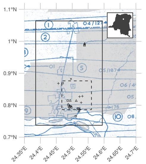
Figure 2.
Overview of the historical flight paths during aerial photo acquisition and ancillary data used in this study: The bounding box of the orthomosaic data presented in this study is shown as a rectangle (23 × 36 km). The outline of a recent high-resolution Geo-Eye panchromatic image is shown as a dashed dark grey rectangle (10 × 10 km). The location of various permanent sampling plots are shown as x, +, and open squares and triangles for the mixed, mono-dominant, and edge plots, respectively. The grey polygon delineates the current-day Yangambi Man and Biosphere reserve. The inset, top right, situates the greater Yangabmi region (white rectangle) within the DR Congo. The full flight plan and details are shown in Appendix A Figure A1 and Figure A2.
2.3. Digitization and Data Processing
All selected images covering the Yangambi area were contact prints as original negatives of the prints were not available. Images were scanned at a resolution exceeding their original resolution (or grain) at the maximal physical resolution of an Epson A3 flatbed scanner (i.e., 2400 dpi or 160 MP per image) and saved as lossless tiff images. Data were normalized using contrast limited histogram equalization [33] with a window size of 32 and a clip limit of 1.5. Fiduciary marks were used to rectify and downsample the images into square 7700 × 7700 pixel images (~1200 dpi, 81 MP). This resulted in a dataset with digital images at a resolution that remained above the visible grain of the photographs, whilst the reduced image size facilitated easier file handling and processing speed.
Data was processed into a georeferenced orthomosaic using a structure-from-motion (SfM, Ullman [34]) approach implemented in Agisoft Metashape version 1.5.2 (Agisoft LLC, St. Petersburg, Russia). An orthomosaic corrects remote sensing data to represent a perfectly downward-looking image, free from perspective distortions due to topography and camera tilt. Using the SfM technique features, areas in images with a large degree of similarity are matched across various images to reconstruct a three-dimensional scene (topography) from two-dimensional image sequences. During the SfM analysis, we masked most clouds, glare, or large water bodies such as the Congo river.
We calculated the orthomosaic using a low-resolution point cloud and digital elevation map (DEM). Additional ground control points were provided to assist in the referencing of image and to constrain the optimization routine used in the SfM algorithm. Ground control points consisted of permanent structures which could be verified in both old and new aerial imagery (i.e., ESRI World Imagery) and consisted of corner points of build structures (e.g., a building, bridge, or swimming pool etc.). Although most clouds were removed during the SfM routine, some were retained to provide sufficient SfM tie points to maximize continuous forest coverage in the final orthomosaic. The final scene was cropped to provide consistent wall-to-wall coverage of the reconstructed scene. The orthomosaic was exported as a geotiff for further georeferencing in QGIS [35] using the georeferencer plugin (version 3.1.9) and additional ESRI World Imagery high-resolution reference data. We used 3rd degree polynomial and 16 ground control points to correct the final image. Ground control points, raw image data, and final processed image are provided in addition to measures of uncertainty such as mean and median error across all ground control points. All subsequent analyses are executed on the final geo-referenced orthomosaic or subsets of it.
2.4. Land-Use and Land-Cover Change
2.4.1. Classifying Land-Use and Land-Cover
Model Training
We automatically delineated all natural forest in the historical data, thus excluding tree plantations, thinned or deteriorated forest stands which showed visible canopy cover loss, fields, and buildings. We used the Unet Convolutional Neural Net (CNN, Ronneberger et al. [36]) architecture implemented in Keras [37] with an efficientnetb3 preprocessing backbone [38] running on TensorFlow [39] to train a binary classifier (i.e., forest or non-forested). Training data were collected from the orthomosaic by randomly selecting 513-pixel square tiles from locations within homogeneous forested or non-forested polygons in the historical orthomosaic (Figure 3). Separate polygons were selected for training, testing, and validation purposes. Validation polygons were sampled 300 times, while both testing and validation polygons were sampled at 100 random locations. Tiles extracted from locations close to the polygon border at times contained mixed cover types. Tiles with mixed cover types were removed from the list of source tiles (Table 1). Homogeneous source tiles were combined in synthetic landscapes using a random Gaussian field-based binary mask (Figure 4). We generated 5000 synthetic landscapes (balancing forest and non-forest classes) for training, while 500 landscapes were generated for both the validation and the testing datasets for a total of 6000 synthetic landscapes. In order to limit stitch line misclassifications, along the seams of mosaicked images, we created synthetic landscapes with different forest tiles to mimick forest texture transitions. We applied this technique to 10% of the generated synthetic landscapes (across training, validation, and testing data).
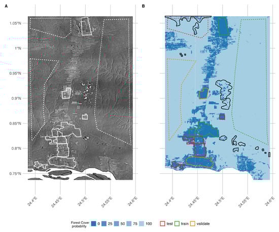
Figure 3.
Overview of the final orthomosaic of the greater Yangambi region (A) as well as the forest cover classification uncertainty (B) used to generate the final land cover map (see Figure 5): Homogeneous polygons used in the generation of the synthetic landscape for convolutional neural network training, testing, and validation are marked as dashed and full lines for forest and non-forest regions, respectively. Training, testing, and validation regions are denoted in panel B in green, red, and orange, respectivelly. Black polygon outlines denote cloud and image stitch line regions which were manually excluded from analysis but retained in calculation of validation statistics (see Table 2).

Table 1.
Number of source tiles used for the generation of synthetic landscapes.
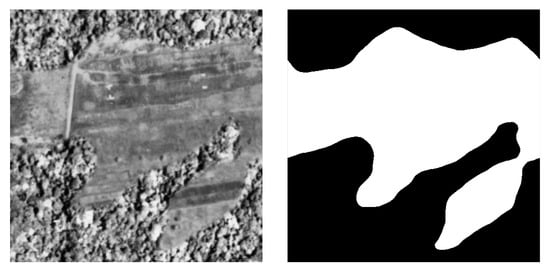
Figure 4.
An example synthetic landscape, combining homogeneous forest and non-forest images into a patchy landscape using random Gaussian field-based masks: The left panel shows a combined synthetic landscape, while the right panel shows the corresponding forest (black) and non-forest (white) labels.
The CNN model was trained for 100 epochs with a batch size of 30 using Adam optimization [40], maximizing the Intersect-over-Union (IoU) using Sørensen–Dice [41] and categorical cross-entropy loss functions. Data augmentation included random cropping to 320-pixel squares, random orientation, scaling, perspective, contrast and brightness shifts, and image blurring. The optimized model was used to classify the complete orthomosaic using a moving window approach with a step size of 110 pixels and a majority vote (>50% agreement) across overlapping areas to limit segmentation edge effects. In addition, we provide raw pixel level classification agreement data for quality control purposes (see data availability below). We refer to Figure 6 for a synoptic overview of the full deep learning workflow.
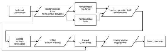
Figure 6.
A diagram of the deep learning workflow followed in training a binary forest/non-forest cover convolutional neural net U-Net model to generate our forest cover map.
Model Validation
We report the CNN accuracy based upon the IoU of our out-of-sample validation dataset of synthetic landscapes. In addition, we report confusion matrices for all pixels across the homogeneous validation polygons as well as the training and testing polygons (see Figure 3). Furthermore, we used the first acquisition of a recent panchromatic Geo-Eye 1 stereo pair (Geo-Eye, Thornton, Colorado, U.S.A., order 737537, 2011-11-11 08:55 GMT or 09:55 local time) to classify and assess the robustness of the CNN algorithm on contemporary remote sensing imagery with similar spectral and spatial characteristics. We used the Global Forest Change version 1.6 (GFC, tile 10N-020E) [1] map data, capturing deforestation up to 2011, to quantify accuracy on downsampled CNN Geo-Eye classification results. Once more, we report the confusion matrix between the GFC- and CNN-derived forest cover maps, masking clouds, and cloud shadows. To summarize confusion matrices, we report accuracy as follows:
where TP, TN, FP, and FN are true positive, true negative, false positive, and false negative, respectively.
2.4.2. Characterizing Long-Term Change
To map long-term LULCC in the Yangambi region, we used the contemporary Global Forest Change version 1.6 (GFC, tile 10N-020E) (lossyear) map data [1]. Using the GFC data, we calculated the latest state of the forest with respect to the conditions at the start of 1958, 60 years earlier. In our analysis, we only included GFC pixels which recorded no forest loss throughout the whole 2000–2018 period. Forest loss in the context of GFC is defined as “a stand-replacement disturbance or a change from a forest to non-forest state”. As such, locations which would see reforestation or deforestation between 2000 and 2018 would be marked as non-forest (i.e., disturbed). As the resolution of the historical forest classification exceeds that of the GFC map, we downsampled our historical forest cover data to 30 m GFC resolution using a nearest neighbour approach. We masked out all water bodies using the Global Forest Change survey data mask layer and limited the analysis to the right bank of the Congo river. We provide summary statistics of historical and contemporary deforestation and reforestation. We map permanent deforestation after 1958, reforestation after 1958, recent deforestation, and long-term (stable) forest cover. All references to changes over time in the context of our analysis explicitly compare the historical and contemporary periods from hereon forth.
2.4.3. Landscape Fragmentation and Aboveground Carbon Estimates
To quantify changes in the structure of forest cover and its disturbances, we used spatial landscape pattern analysis (i.e., fragmentation) metrics [42]. Landscape metrics provide a mathematical framework for the analysis of discrete land-cover classes and allows us to capture their composition and configuration. These metrics are therefore commonly used to compare how landscapes change over time [43]. In particular, fractals provide a way to quantify complex natural landscapes, including their self-similarity across scales [44,45]. We report the ratio of edge to area and the fractal dimension to quantify landscape complexity of forest disturbances. A fractal dimension closer to 2 suggests a more complex (fragmented) landscape.
Statistics were calculated for all forest disturbance patches larger than 1 ha and smaller than the 95th percentile of the patch size distribution using the R package “landscapemetrics” [43]. We provide mean and standard deviation on edge, area, their ratio, and fractal dimension for both the historical and contemporary Hansen et al. [1] forest cover maps.
We estimated aboveground carbon (AGC) losses and gains due to deforestation and reforestation using plot-based averages of recent inventory data at permanent sampling plots in the area (Figure 2). We refer to Kearsley et al. [30] for the survey method and allometric relations used to scale the survey data. Unlike standard square 1 ha plots, edge plots (163.03 ± 19.39 Mg C ha−1, N = 5) were set back 200 m from forest edges and were 50 × 200 m, with the 50 m side of the plot along the forest edge and continuing 200 m into the forest (Appendix A Table A2). We further confirmed that forest edge plots, as compared to mixed forest plots (160.48 ± 23.84 Mg C ha−1, N = 8, see Appendix A Table A3 for all forest types) did not show a significantly different AGC (Mann Whitney U test, p < 0.05). Thus, it was not necessary to explicitly quantify changes in AGC caused by edge effects. Moreover, we used the mean value and its uncertainty (i.e., standard deviation) of the mixed forest as representative for potential AGC losses. Despite the challenges inherent in quantifying AGC for forest edges, we mapped the total extent of the edges in the contemporary landscape. To align our landscape analysis with exploratory analysis of the survey data, we used a buffer of 200 m to estimate the extent of forest edges and patches up to the location of forest edge plots.
Surveys of old plantations show a large variation in AGC, depending on age and the crop type. For example, the AGC values varied from 86.55 to 168.67 Mg C ha−1, for Elaeis guineensis (oil palm) and Hevea brasiliensis (rubber tree) plots, respectively (Bustillo et al. [46], personal communications). These higher values are in line with the mixed plot AGC estimates (160.48 ± 23.84 Mg C ha−1, N = 8) in the area, while the palm plantations resemble old-regrowth values (81.87 Mg C ha−1, N = 1). To quantify AGC in reforested areas, we therefore use both AGC estimates of old-regrowth and mixed forest as lower and upper bounds. We did not have sufficient data to account for individual changes in AGC across plantations.
2.5. Canopy Structure and FOTO Texture Analysis
We compared the structure of the canopy both visually and using Fourier Transform Textural Ordination (FOTO, Couteron [47]). FOTO uses a principal component analysis (PCA) on radially averaged 2D Fourier spectra to characterize canopy (image) texture. The FOTO technique was first described by Couteron [47] to quantify canopy stucture in relation to biomass and biodiversity and can be used across multiple scenes using normalization [16].
We used the standard FOTO methodology with fixed zones instead of the moving window approach. The window size was set to the same size (187 pixels or ~150 m) as used in the moving window analysis above. To account for illumination differences between the two scenes, we applied histogram matching. No global normalization was applied, as the scene was processed as a whole. PC values from this analysis for all permanent sampling plots in both image scences were extracted using a buffer with a radius of 50 m.
For both site-based and scene analysis, we correlated PC values with permanent sample plot inventory data such as stem density, aboveground biomass, and tree species richness (Appendix A Table A2 and Table A3). Additional comparisons are made between contemporary Geo-Eye data and the historical orthomosaic-derived PC values. Due to the few available permanent sampling plots in both scenes, we used a nonparametric paired signed rank (Wilcoxon) test [48] to determine differences between the PC values of the Geo-Eye and historical orthomosaic image scenes across mono-dominant and mixed forest types. In all analysis, mono-dominant site 4 was removed from the analysis due to cloud contamination.
3. Results
3.1. Orthomosaic Construction
Our analysis provides a first spatially explicit historical composite of aerial survey images in support of mapping land-use and land-cover within the Congo Basin. The use of high-resolution historical images combined with SfM image processing techniques allowed us to mosaic old imagery across a large extent. The final orthomosaic composition of the Yangambi region provided an image scene covering approximately 733 million pixels across ~93,431 ha with a resolution of 0.88 m/pixel (or ~23 × 36 km, Figure 2). The overall spatial accuracy of the SfM orthomosaic composition using the sparse cloud DEM (with a resolution of 45.8 m/pixel) was limited to approximately 23 m. Further georeferencing outside the SfM workflow reduced the mean error at the ground control points to 5.3 ± 4.9 px (~4.7 ± 4.3 m), with a median error of 2.9 px (2.6 m). The orthomosaic served as input for all subsequent LULCC analysis with all derived maps provided with the manuscript repository (see data and code availability statements below).
3.2. Land-Use and Land-Cover Classification
CNN Model Validation
The CNN deep learning classifier reached an intersection-over-union accuracy of 97% on the detection of disturbed forest in the out-of-sample (validation) synthetic landscape data. Using all pixels within the validation polygons (Figure 3) showed a similar accuracy value of ~98%. Using all polygons across the scene, including those used in the generation of testing and training synthetic landscapes, increased the accuracy to ~99% (Table 2). A comparison with recent panchromatic Geo-Eye data shows good agreement, with an accuracy of ~87% across all pixels between the landsat-based GFC data and downscaled CNN results (Table 2 and Figure 7).
Table 2.
Confusion matrix showing % agreement between forest/non-forest classes using a Convolutional Neural Network (CNN) across previously selected homogenous areas: In addition, overall accuracy is reported for each confusion matrix.
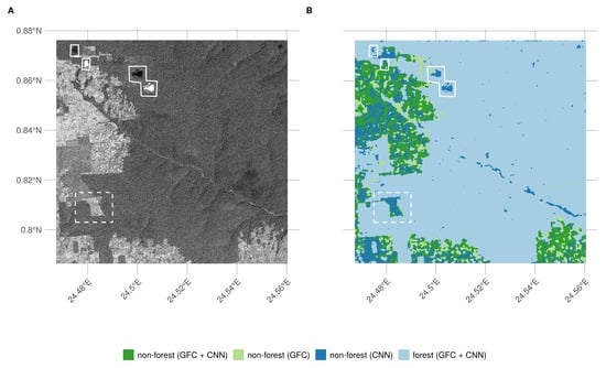
Figure 7.
Convolutional Neural Network (CNN)-based forest cover classification results (B) as run on a recent (2011) Geo-Eye panchromatic image (A): We show the difference between the convolutional neural network-based classification and a recent Landsat-based forest cover map by Hansen et al. 2013. Full white outlines denote cloud contamination; the dashed rectangle shows a location where the CNN outperforms the Landsat based forest classification.
3.3. Long-Term Changes in LULC and Aboveground Carbon
Scaling our classifier to the whole historical orthomosaic, we detected ~16,200 ha (or ~20% of the scene) of disturbed forests. A large fraction of the disturbed area was restored in the period between the two acquisition periods. In total, 9918 ha, or little over half of the affected forest, was restored (Figure 3C,D, dark blue). Recent deforested areas, as registered through satellite remote sensing (>2000), approximate 8776 ha (Table 3, Figure 5, light green).
Table 3.
Land-use land-cover change statistics of forest cover around Yangambi in the central Congo Basin: The data evaluates a difference between a historical (1958) aerial photography-based survey and the Hansen et al. 2013-based satellite remote sensing data. Spatial coverage statistics are provided hectares (ha), rounded to the nearest integer as well as Above Ground Carbon (AGC) scaled using recent survey measurements. Both non-forest cover in 1958 and the forest edge area are subsets of the original data (see Figure 5) and do not count toward the total scene area.
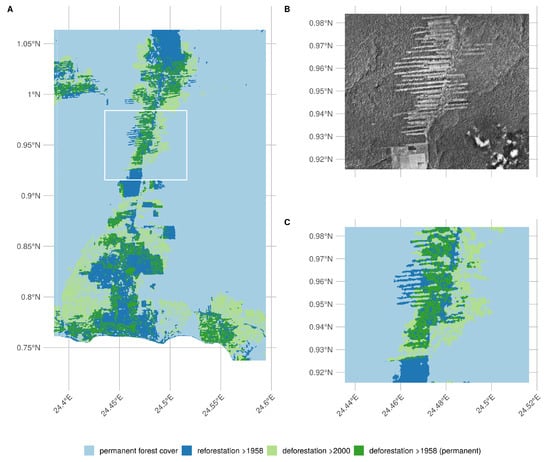
Figure 5.
Overview of the final land-use land-cover change map (A), a detailed inset of both the underlying orthomosaic (B) and the derived land-use land-cover change map displayed as the difference between the convolutional neural network-based classification orthomosaic and the recent Landsat-based forest cover map by Hansen et al. 2013 (C).
Recent deforestation follows a distinctly different pattern compared to historical patterns. Historical deforestation showed a classical fishbone pattern for forest clearing with very sharp edges, while current patterns are patchy and ad hoc (Figure 5C, dark blue and green colours, respectively). These differences are reflected in the analysis of landscape metrics of deforestation. Between the historical and contemporary LULCC maps, we see an increase in small disturbances, as indicated by the decreasing area of the mean patch size, down to ~1.86 ± 0.75 ha from ~5.25 ± 5.02 ha historically. Perimeter lengths were longer historically, at 1451 ± 943 m, compared to contemporary landscapes ~921 ± 362 m (Table 4). This shift in perimeter area ratio led to a similar change in the fractal index, slightly increasing in value to 1.1 ± 0.05 from 1.09 ± 0.04 over time. Values closer to a fractal index of 2 suggest a more complex (fragmented) landscape.
Table 4.
Landscape metrics for historical and contemporary deforestation patterns: We report patch perimeter and area, their ratio, and fractal dimension. Values are reported as mean ± standard deviation across all deforestation patches.
A comparison of forest edge plots with mixed forest plots showed no signficant difference in AGC or other reported values such as species richness, basal area, or stem density (Mann Whitney U test, p < 0.05). Edge influence did not extend beyond 200 m from a forest edge but still represented an area of 13,151 ha (Table 3).
Changes in both land use and land cover led to concomitant changes in AGC stocks. Recovery throughout the region was characterized for patches of forest and plantations. Assuming high density stands, based on previous work, this could amount to a carbon gains of up to 1592 Gg C across our study area, offsetting more recent losses of approximately 1408 ± 209 Gg C. On the other hand, at the low end, if we assume a lower carbon density of 81.8 Mg C ha−1, this would result in a total carbon gain of 811 Gg C. Using our approach, results indicate that overall deforestation around Yangambi has resulted in a loss of ~2416 ± 358 Gg C in AGC stocks.
3.4. Canopy Structure and FOTO Texture Analysis
Visual interpretation of the scenes provide evidence that most locations do not change dramatically with respect to canopy composition, except for the large areas of disturbances in contemporary fallow or young-regrowth plots. One marked difference is noted in the mono-dominant plot 6 (Appendix A Table A2). Here, the current mono-dominant Brachystegia laurentii is a recent development, changing the canopy structure visibly during the last half century (Figure 8). The previous varied canopy structure gave way to a more dense and uniform canopy. This is reflected in a change of the FOTO PC value from 0.19 historically to its current value of 0.54 (Figure 9). This historical value is similar to the mean of contemporary mono-dominant stands of Gilbertiodendron dewevrei with PC averaging 0.34 ± 0.1 and is only slightly higher than historical values for a mixed forest (0.18 ± 0.08, Figure 9). The reverse pattern is seen in the contemporary PC values. Here, the value of 0.54 exceeds those of most mono-dominant stands (0.35 ± 0.08) and is even further removed from the values noted for mixed forests (0.12 ± 0.03, Figure 9).
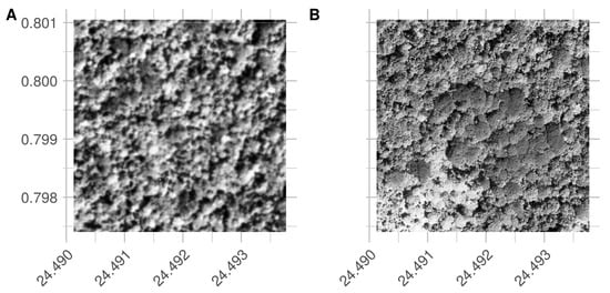
Figure 8.
Visual comparison between a historical (A) and contemporary (B) permanent sampling plot. The site is currently listed as a mono-dominant Brachystegia laurenttii stand: Note the structural differences with a “courser” canopy structure in the historical image compared to the more closed contemporary stand.
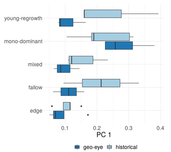
Figure 9.
Boxplots comparing the first principal component (PC1) of a site-based Fourier Transform Textural Ordination (FOTO) analysis across different forest types for both contemporary (Geo-Eye) and historical orthomosaic data.
Using only small subsets around existing permanent sampling plots, we show distinct differences between forest types, with PC values in both historical and contemporary imagery markedly higher for the mono-dominant forest types compared to all others (Appendix A Figure A4). Provided that the young-regrowth and fallow permanent sampling plots have seen recent disturbance, the Wilcoxon signed rank test on the mixed and mono-dominant plots between the historical and contemporary PC values did not show a significant difference (p > 0.05). Similarly, no significant different using PC values extracted from the whole scene analysis was noted (p > 0.05). Any relationships between contemporary Geo-Eye data and permanent sampling plot measurements of aboveground carbon, stem density, and species richness were nonsignificant (p > 0.05, Appendix A Figure A4, Figure A5 and Figure A6).
Furthermore, visual inspection of the scene-wide analysis suggests historical scences do not show landscape-wide canopy features (Figure 10A,B), unlike the contemporary scene (Figure 10C,D). In the contemporary scene, the FOTO algorithm picks up landscape features such as changes in texture along the river valley (the diagonal line in Figure 10D). However, no corresponding landscape patterns are found by the FOTO algorithm in the historical orthomosaic.
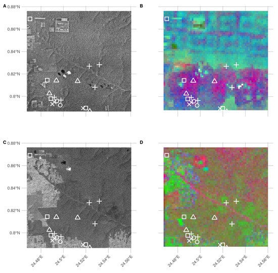
Figure 10.
Black and white overview images and red-green-blue (RGB) visualizations of the first three principal components of scene-wide FOTO texture analysis of historical (A,B) and current (Geo-Eye, C,D) imagery: Current permanent sampling plots of mono-dominant, mixed, fallow, and young (edge) forest plots are marked with open triangles, open circles, open squares, and crosses, respectively.
4. Discussion
Finely grained spatial data sources, such as remote sensing imagery, are rare before the satellite era (<1972). This lack of data limits our understanding of how forest structure has varied over longer time periods in remote areas. Long-term assessment can be extended by using large inventories of historical aerial survey data [22,23,49]. Despite the difficulties in recovering this data and its limitations, such as invisible disturbances [50], remote sensing generally remains the best way to map and quantify LULCC [2]. In our study, we used novel numerical remote sensing techniques to valorize, for the first time, historical remote sensing data in order to quantify (long term) land-use and land-cover change and canopy structural properties in the central Congo Basin. Despite these successes, some methodological and research considerations remain.
4.1. Methodological Considerations
4.1.1. Data Recovery Challenges
In our study, the archive data recovered was limited to contact prints and therefore did not represent the true resolution of the original negative. In addition, analogue photography clearly produces a distinct softness compared to digital imagery (Figure 8). Despite favourable nadir image acquistions [51], image softness combined with illumination effects between flight paths and the self-similar nature of vast canopy expanses [52,53,54] limited our ability to provide wall-to-wall coverage of the entire dataset containing 334 images. A few man-made features in the scenes also made georeferencing challenging. Although the village of Yangambi provided a range of buildings as (hard-edge) references, other areas within the central Congo Basin might have fewer permanent structures and would require the use of soft-edged landscape features (e.g., trees and river outflows). Research has shown that soft-edged features can help georeference scenes even when containing few man-made features [55]. Our two-step georeferencing approach resulted in a referencing accuracy of ~4.7 ± 4.3 m across reference points. However, it shoud be noted that referencing accuracy of the final scene is less constrained toward the edges of the scene.
4.1.2. LULC Classification and Validation
When classifying the orthomosaic into forest and non-forest states, we favoured a deep-learning-supervised classification using a CNN over manual segmentation to guarantee an “apples-to-apples” comparison between the historical and the contemporary GFC forest cover map used in our analysis. We acknowledge that both the CNN and GFC land-use and land-cover maps use different underlying features, i.e., spatial or spectral data, yet attain a similarly high accuracy of up to 99% [1]. More so, when validating our CNN classifier against GFC data (Figure 7) for a contemporary high-resolution Geo-Eye panchromatic image, we reach an accuracy of ~87%, despite a time difference of almost 60 years. Visual inspection of the classification data in Figure 7 suggests that the GFC map more often than not classifies non-forest areas as forest. Actual classification accuracy of our algorithm might therefore be higher than our reported value.
4.1.3. Scaling Opportunities
Our approach uses broadly defined homogeneous polygons to construct a balanced dataset of synthethic landscapes. The methodology is analoguous to the use of sparse labelling as used by Buscombe and Ritchie [56] and contrasts with the standard methodologies which generally extract pixel (windows) [22] or delineate land cover classes [23] to drive a classifier or analysis. More so, the use of heavy image augmentation during model training sidesteps texture representation issues which affect classification of image scenes with inconsistent illumination or sharpness [25] or ad hoc feature engineering [22]. The use of synthetic landscapes allowed us to account for most, but not all, of the variability within our orthomosaic. Our analysis has shown that, despite being trained on historical data, our model could map contemporary forest cover in remote sensing data with similar spatial and spectral characteristics (Figure 7), suggesting that the classifier consistently works across both space and time. We acknowledge that the use of synthetic landscapes is limited by the available homogeneous areas to sample from and the number of classes. However, the latter should not be a constrained as previous research efforts have focussed on simple forest cover maps [1].
4.2. Research Context
4.2.1. Long Term Changes in LULC and Aboveground Carbon
Our analysis shows that the majority of deforestation around Yangambi happened toward the late 1950s (~16,200 ha). Considerable reforestation has occured since the aerial survey was executed (~9918 ha), and socioeconomic instability prevented further large scale forest exploitation. In particular, many plantations have reached maturity, and forest has reestablished in previously cleared or disturbed areas. The majority of this reforestation takes the form of isolated patches of forest but is offset by further deforestation of previously untouched forest. Generally, the function and structure of forests can be influenced by forest edges that are located up to 1 km away; however, most effects are pronounced within the first 300 m from the edge [57]. Our analysis of edge effects on AGC has shown that the influence is negligible 200 m away from the edge. Phillips et al. [58] have shown similar weak responses to edge effects in the Amazon forest. Due to a lack of data on the extent (depth) of edge effects and their influence on AGC beyond 200 m, we did not include any estimates of carbon loss or gain within these zones. However, it must be stated that edges throughout the landscape make up a substantial area and account for 13,151 ha. Thus, edges could have a substantial negative [6] or positive [59] influence on AGC. Similarly, uncertainties in how to explicitly correct for plantations in the landscape present a further challenge. Similarly, variability across mixed forest plots used in scaling aboveground carbon estimates due to deforestation introduced additional uncertainty (see Appendix A Table A3). Thus, although our estimates are only indicative, they do underscore the important influence of landscape structure in carbon accounting. However, our findings do not indicate that deforestation in Congo Basin is declining, on the contrary.
Over the past half century, there has been a clear shift in land use in Yangambi (Figure 3). Land use has shifted away from a regular (fishbone) deforestation pattern that emerges when (large scale) agricultural interests dominate the landscape [60] to a more fragmented landscape (Figure 3D). The former is consistent with historical land management at the time of the aerial survey [46]. These regular patterns reversed due to a decrease in large-scale intensive agriculture and an increase in ad hoc small-scale subsistence farming with large perimeter-to-area relationships (i.e., ragged edges). Consequently, edge effects in the current landscape are far more pronounced than in the historical scene.
Visual inspection of the images also suggests that reforestation within the historically cleared areas and experimental plots is not necessarily limited to areas far removed from more densely populated areas. For example, large reforested areas exist close to the Congo stream and Yangambi village itself (Figure 3). Here, regional political components, such as land leases and large-scale ownership could have played a role in safeguarding some of these areas for rewilding or sustainable management [61,62]. Despite widespread anthropogenic influences throughout the tropics [31], the retention of these forested areas show the potential of explicit or implicit protective policy measures (e.g., INERA concessions, Bustillo et al. [46]) on a multi-decadal time scale. Reforestation in noncontinuous areas within Yangambi could increase landscape connectivity and could help increase biodiversity [12].
Our analysis therefore provides an opportunity to highlight and study those regions that have previously suffered confirmed long-term disturbances and those that have been restored since. Assessments of old plantations and recovering clear-cut forests can serve as a guide to help estimate carbon storage capacity and forest recovery rates in managed and unmanaged conditions [18,20,63] over the mid to long term in support of rewilding and general forest restoration [12,61,62]. In addition, mapping long-term edge effects can further support research into issues such as receding forest edges [57].
4.2.2. Canopy Structure and FOTO Texture Analysis
Finally, the FOTO technique used to quantify relationships between canopy structure and forest characteristics rendered no valuable insights of either the historical orthomosaic or recent Geo-Eye scene. Similarly weak correlations were found previously by Solórzano et al. [64]. In contrast, site-based texture metric statistics did show correspondence between historical and contemporary satellite imagery. None of them were either consistent or significant. Although visual interpretation shows distinctly different canopy structures (Figure 3), the differences in how resolution is defined and issues related to image quality prevented us from quantifying these further. Unlike large-scale studies by Ploton et al. [14], we could not scale this technique to historical data. The successful use of our CNN classification model on a contemporary remote sensing data does suggest that texture can be used to consistently capture canopy properties 60 years apart. Differences in PC between forest types (e.g., mono-dominant vs. mixed, Figure 9) corroborate that texture can serve as a basis for LULC classification. However, inflexibility on part of the FOTO technique in dealing with non-standardized (historical) data or scaling these results to AGC values limits its use case. We advise that future valorisation efforts should preferentially work from FOTO negatives (if available) to ensure optimal data quality in resolution, contrast, and sharpness.
5. Conclusions
Given the impact of tropical forest disturbances on atmospheric carbon emissions, biodiversity, and ecosystem productivity, accurate long-term reporting of LULCC is an imperative. Our analysis of historical aerial survey images (1958) of the Central Congo Basin provides a window into the state of the forest at the start of the anthropocene. The use of a CNN-based LULC classifier using synthetic landscapes-based image augmentation provides a robust semi-supervised solution which scales across space and time, even for image scenes with inconsistent illumination or sharpness. Combined with contemporary remote sensing data, we have shown that historical aerial survey data can be used to quantify long-term changes in LULC and AGC. We showed a shift from previously highly structured industrial deforestation of large areas for plantation purposes to discrete smallholder clearing for farming, increasing landscape fragmentation and opportunties for substantial regrowth. Efforts to quantify canopy texture features and their link to AGC had limited to no success. Our analysis provides insights into the rate at which deforestation and reforestation has taken place over a multi-decadal scale in the central Congo Basin. As such, it provides a useful historical context while interpreting past and ongoing forest research in the area.
6. Additional Information and Declarations
6.1. Data Availability
Hufkens et al. (2019): A curated dataset of aerial survey images over the central Congo Basin, 1958. Zenodo: https://doi.org/10.5281/zenodo.3547767. All data not included in the latter repository can be found bundled with the analysis code as listed below. Proprietary datasets (i.e., Geo-Eye data) are not shared, but purchase order numbers allow for acquisition of these datasets to ensure reproducibility.
6.2. Code Availability
All analysis code is available as R/python [65] projects (https://khufkens.github.io/orthodrc and https://khufkens.github.io/orthodrc_cnn/). The analysis relied heavily on the “raster” [66], “RStoolbox” [67], and “landscapemetrics” [43] packages, while post-processing and plotting was facilitated by the “tidyverse” ecosystem [68], “ggthemes” [69], “scales” [70], and “cowplot” [71]. Additional plotting elements were formatted or provided by “sf” [72] and “rnaturalearth” [73] packages. I am grateful for the contributions to the scientific community by the developers of these packages.
Author Contributions
K.H. conceived and designed the study, analyzed the data, prepared figures and tables, and authored the final draft of the manuscript. T.d.H. scanned all image data. E.K. and T.d.H. provided plot-based AGC estimates. T.d.H., K.J., E.K., H.B., P.S., F.V., S.M., M.A., J.V.d.B., H.V., L.V.H. and L.W. reviewed the final manuscript. All authors have read and agreed to the published version of the manuscript.
Acknowledgments
This research was supported through the Belgian Science Policy office COBECORE project (BELSPO; grant BR/175/A3/COBECORE). K.H. acknowledges funding from the European Union Marie Skłodowska-Curie Action (project number 797668). K.H. is grateful for the support of T.d.H. volunteering his time in scanning the images.
Conflicts of Interest
The authors declare no conflict of interest. The founding sponsors had no role in the design of the study; in the collection, analyses, or interpretation of data; in the writing of the manuscript; or in the decision to publish the results.
Appendix A
Table A1.
Flight path meta-data for the Isangi-Stanleyville aerial survey. Data provided consists of the flight path number, cardinal direction of the flight, the image numbers, and the duration of the flight provided by the start and end time of the acquisition. Data is sourced from Appendix A Figure A2 and the sensor logs recorded in the margin of acquired images (see Figure 1 main manuscript).
| Path | Direction | Image # | Start (H:M:S) | End (H:M:S) |
|---|---|---|---|---|
| 1 | W – E | 04 / 78 – 04 / 127 | 10:15:00 | 10:40:00 |
| 2 | W – E | 05 / 01 – 05 / 56 | 10:15:00 | 10:40:00 |
| 3 | W – E | 06 / 01 – 06 / 48 | 08:55:00 | 09:20:00 |
| 4 | W – E | 07 / 01 – 07 / 20 | 09:30:00 | 09:45:00 |
| 5 | W – E | 05 / 167 – 05 / 187 | 08:55:00 | 09:10:00 |
| 6 | W – E | 07 / 67 – 07 / 82 | 10:50:00 | 11:00:00 |
| 7 | E – W | 06 / 49 – 06 / 95 | 09:35:00 | 10:05:00 |
| 8 | E – W | 05 / 57 – 05 / 103 | 10:20:00 | 10:50:00 |
| 9 | E – W | 04 / 128 – 04 / 176 | 10:50:00 | 11:10:00 |
| 10 | W – E | 08 / 01 – 08 / 27 | 09:05:00 | 09:20:00 |
| 11 | W – E | 06 / 96 – 06 / 139 | 10:25:00 | 10:45:00 |
Table A2.
Site description of all the current permanent sampling plots in the greater Yangambi region. We list the forest type, plot number, geographic location (in decimal degrees), stem density, basal area Above Ground Carbon (AGC), species richness and Land-Use and Land-Cover Change (LULCC) classes in a radius of 100 m around each plot location.
| Type | nr | Latitude | Longitude | Stem Density (ha−1) | Basal Area (m2 ha−1) | AGC (Mg C ha−1) | Species Richness | LULCC Class Coverage (%) |
|---|---|---|---|---|---|---|---|---|
| fallow | 1 | 0.7959139 | 24.49423 | 350 | 5.39000 | 6.7000 | 26 | 37 (1), 63 (3) |
| fallow | 2 | 0.7921028 | 24.49717 | 132 | 2.06000 | 2.0400 | 22 | 68 (1), 32 (3) |
| young-regrowth | 1 | 0.7894028 | 24.51755 | 322 | 20.44000 | 46.5600 | 40 | 68 (1), 32 (3) |
| young-regrowth | 2 | 0.7948806 | 24.49193 | 447 | 16.63000 | 27.8300 | 25 | 56 (1), 44 (3) |
| young-regrowth | 3 | 0.7931083 | 24.49013 | 313 | 17.80000 | 37.1000 | 43 | 51 (1), 49 (3) |
| old-regrowth | 1 | 0.8824444 | 24.49614 | 384 | 19.48000 | 81.7800 | 92 | 100 (1) |
| mixed | 1 | 0.8135486 | 24.51264 | 563 | 34.81000 | 168.0400 | 83 | 100 (1) |
| mixed | 2 | 0.7805000 | 24.52109 | 403 | 35.25000 | 174.5800 | 78 | 100 (1) |
| mixed | 3 | 0.7866181 | 24.52349 | 367 | 30.69000 | 150.3000 | 75 | 100 (1) |
| mixed | 4 | 0.8140333 | 24.49370 | 432 | 33.01000 | 168.6100 | 84 | 100 (1) |
| mixed | 5 | 0.8025611 | 24.48750 | 329 | 25.20000 | 124.1800 | 80 | 100 (1) |
| mixed | 6 | 0.9925556 | 24.53906 | 490 | 32.63000 | 203.8100 | 86 | 100 (1) |
| mixed | 7 | 0.9898056 | 24.53853 | 598 | 31.47000 | 146.1100 | 92 | 100 (1) |
| mixed | 8 | 0.9866111 | 24.53856 | 556 | 29.20000 | 148.2100 | 90 | 100 (1) |
| mono-dominant | 1 | 0.8269306 | 24.52303 | 344 | 31.80000 | 183.0100 | 48 | 100 (1) |
| mono-dominant | 2 | 0.8282708 | 24.53196 | 436 | 32.06000 | 173.5800 | 55 | 100 (1) |
| mono-dominant | 3 | 0.7965903 | 24.49779 | 376 | 30.57000 | 166.4400 | 62 | 100 (1) |
| mono-dominant | 4 | 0.8080889 | 24.52811 | 374 | 27.69000 | 145.5500 | 46 | 100 (1) |
| mono-dominant | 5 | 0.8682806 | 24.45655 | 217 | 27.19000 | 159.0000 | 46 | 95 (1), 5 (2) |
| mono-dominant | 6 | 0.7992278 | 24.49195 | 378 | 33.95000 | 165.4800 | 68 | 100 (1) |
| edge | 1 | 0.7895486 | 24.51990 | 415 | 30.93601 | 152.2792 | 77 | 100 (1) |
| edge | 2 | 0.7979472 | 24.48885 | 368 | 31.82097 | 152.1736 | 72 | 95 (1), 5 (3) |
| edge | 3 | 0.8144250 | 24.48555 | 458 | 35.79959 | 197.4022 | 86 | 100 (1) |
| edge | 4 | 0.7659306 | 24.51125 | 320 | 29.72547 | 154.6380 | 75 | 98 (1), 2 (3) |
| edge | 5 | 0.8691778 | 24.47019 | 459 | 33.72462 | 158.6934 | 88 | 100 (1) |
Table A3.
Summary statistics for different forest plot types. We report the mean and standard deviation for Above Ground Carbon (AGC), basal area, stem density values and number of plots (as mentioned in Appendix A Table A1).
Table A3.
Summary statistics for different forest plot types. We report the mean and standard deviation for Above Ground Carbon (AGC), basal area, stem density values and number of plots (as mentioned in Appendix A Table A1).
| Forest Type | AGC (Mg C ha−1) | Stem Density (ha−1) | Basal Area (m2 ha−1) | nr. plots |
|---|---|---|---|---|
| edge | 163.04 ± 19.39 | 404 ± 60.03 | 32.4 ± 2.39 | 5 |
| fallow | 4.37 ± 3.3 | 241 ± 154.15 | 3.72 ± 2.35 | 2 |
| mixed | 160.48 ± 23.84 | 467.25 ± 99.42 | 31.53 ± 3.26 | 8 |
| mono-dominant | 165.51 ± 12.75 | 354.17 ± 73.56 | 30.54 ± 2.64 | 6 |
| old-regrowth | 81.78 | 384 | 19.48 | 1 |
| young-regrowth | 37.16 ± 9.37 | 360.67 ± 74.9 | 18.29 ± 1.95 | 3 |

Figure A1.
Overview of the complete flight plan of the survey around Kisangani (then Stanleyville) stored in the archives at the Africa Museum.
Figure A1.
Overview of the complete flight plan of the survey around Kisangani (then Stanleyville) stored in the archives at the Africa Museum.


Figure A2.
Overview of the complete flight plan meta-data as stored in the archives at the Africa Museum.
Figure A2.
Overview of the complete flight plan meta-data as stored in the archives at the Africa Museum.


Figure A3.
Shelves with aerial survey images at the Africa Museum archives, showing vasts amounts of historical data still mostly unexplored.
Figure A3.
Shelves with aerial survey images at the Africa Museum archives, showing vasts amounts of historical data still mostly unexplored.


Figure A4.
Scatterplot comparing Above Ground Carbon and the first principal component of the FOTO analysis for contemporary Geo-Eye (left) and the historical orthomosaic (right) data. Different forest types are plotted using closed circles, closed triangles, closed squares and this for fallow, mixed mon-dominant and young-regrowth forests, respectivelly


Figure A5.
Scatterplot comparing tree species richness and the first principal component of the FOTO analysis for contemporary Geo-Eye (left) and the historical orthomosaic (right) data. Different forest types are plotted using closed circles, closed triangles, closed squares and this for fallow, mixed mon-dominant and young-regrowth forests, respectivelly


Figure A6.
Scatterplot comparing stem density (per ha) and the first principal component of the FOTO analysis for contemporary Geo-Eye (left) and the historical orthomosaic (right) data. Different forest types are plotted using closed circles, closed triangles, closed squares and this for fallow, mixed mon-dominant and young-regrowth forests, respectivelly

References
- Hansen, M.C.; Potapov, P.V.; Moore, R.; Hancher, M.; Turubanova, S.A.; Tyukavina, A.; Thau, D.; Stehman, S.V.; Goetz, S.J.; Loveland, T.R.; et al. High-Resolution Global Maps of 21st-Century Forest Cover Change. Science 2013, 342, 850–853. [Google Scholar] [CrossRef]
- Houghton, R.A.; House, J.I.; Pongratz, J.; van der Werf, G.R.; DeFries, R.S.; Hansen, M.C.; Le Quéré, C.; Ramankutty, N. Carbon emissions from land use and land-cover change. Biogeosciences 2012, 9, 5125–5142. [Google Scholar] [CrossRef]
- Tyukavina, A.; Baccini, A.; Hansen, M.C.; Potapov, P.V.; Stehman, S.V.; Houghton, R.A.; Krylov, A.M.; Turubanova, S.; Goetz, S.J. Aboveground carbon loss in natural and managed tropical forests from 2000 to 2012. Environ. Res. Lett. 2015, 10, 074002. [Google Scholar] [CrossRef]
- Van der Werf, G.R.; Morton, D.C.; DeFries, R.S.; Olivier, J.G.J.; Kasibhatla, P.S.; Jackson, R.B.; Collatz, G.J.; Randerson, J.T. CO2 emissions from forest loss. Nat. Geosci. 2009, 2, 737–738. [Google Scholar] [CrossRef]
- Fauset, S.; Gloor, M.U.; Aidar, M.P.M.; Freitas, H.C.; Fyllas, N.M.; Marabesi, M.A.; Rochelle, A.L.C.; Shenkin, A.; Vieira, S.A.; Joly, C.A. Tropical forest light regimes in a human-modified landscape. Ecosphere 2017, 8, e02002. [Google Scholar] [CrossRef] [PubMed]
- Brinck, K.; Fischer, R.; Groeneveld, J.; Lehmann, S.; Dantas De Paula, M.; Pütz, S.; Sexton, J.O.; Song, D.; Huth, A. High resolution analysis of tropical forest fragmentation and its impact on the global carbon cycle. Nat. Commun. 2017, 8. [Google Scholar] [CrossRef] [PubMed]
- Didham, R.K. Edge Structure Determines the Magnitude of Changes in Microclimate and Vegetation Structure in Tropical Forest Fragments. Biotropica 1999, 31, 17–30. [Google Scholar] [CrossRef]
- Laurance, W.F.; Delamônica, P.; Laurance, S.G.; Vasconcelos, H.L.; Lovejoy, T.E. Rainforest fragmentation kills big trees. Nature 2000, 404, 836. [Google Scholar] [CrossRef]
- Magnago, L.F.S.; Magrach, A.; Laurance, W.F.; Martins, S.V.; Meira-Neto, J.A.A.; Simonelli, M.; Edwards, D.P. Would protecting tropical forest fragments provide carbon and biodiversity cobenefits under REDD+? Glob. Chang. Biol. 2015, 21, 3455–3468. [Google Scholar] [CrossRef]
- Poorter, L.; Bongers, F. Leaf traits are good predictors of plant performance across 53 rain forest species. Ecology 2006, 87, 1733–1743. [Google Scholar] [CrossRef]
- Barlow, J.; Lennox, G.D.; Ferreira, J.; Berenguer, E.; Lees, A.C.; Nally, R.M.; Thomson, J.R.; Ferraz, S.F.d.B.; Louzada, J.; Oliveira, V.H.F.; et al. Anthropogenic disturbance in tropical forests can double biodiversity loss from deforestation. Nature 2016, 535, 144–147. [Google Scholar] [CrossRef] [PubMed]
- Van de Perre, F.; Willig, M.R.; Presley, S.J.; Bapeamoni Andemwana, F.; Beeckman, H.; Boeckx, P.; Cooleman, S.; de Haan, M.; De Kesel, A.; Dessein, S.; et al. Reconciling biodiversity and carbon stock conservation in an Afrotropical forest landscape. Sci. Adv. 2018, 4, eaar6603. [Google Scholar] [CrossRef]
- Mitchard, E.T.A. The tropical forest carbon cycle and climate change. Nature 2018, 559, 527–534. [Google Scholar] [CrossRef]
- Ploton, P.; Pélissier, R.; Proisy, C.; Flavenot, T.; Barbier, N.; Rai, S.N.; Couteron, P. Assessing aboveground tropical forest biomass using Google Earth canopy images. Ecol. Appl. 2012, 22, 993–1003. [Google Scholar] [CrossRef]
- Couteron, P.; Pelissier, R.; Nicolini, E.A.; Paget, D. Predicting tropical forest stand structure parameters from Fourier transform of very high-resolution remotely sensed canopy images. J. Appl. Ecol. 2005, 42, 1121–1128. [Google Scholar] [CrossRef]
- Barbier, N.; Couteron, P.; Proisy, C.; Malhi, Y.; Gastellu-Etchegorry, J.P. The variation of apparent crown size and canopy heterogeneity across lowland Amazonian forests. Glob. Ecol. Biogeogr. 2010, 19, 72–84. [Google Scholar] [CrossRef]
- DeFries, R.S.; Houghton, R.A.; Hansen, M.C.; Field, C.B.; Skole, D.; Townshend, J. Carbon emissions from tropical deforestation and regrowth based on satellite observations for the 1980s and 1990s. Proc. Natl. Acad. Sci. USA 2002, 99, 14256–14261. [Google Scholar] [CrossRef]
- Achard, F.; Beuchle, R.; Mayaux, P.; Stibig, H.J.; Bodart, C.; Brink, A.; Carboni, S.; Desclée, B.; Donnay, F.; Eva, H.D.; et al. Determination of tropical deforestation rates and related carbon losses from 1990 to 2010. Glob. Chang. Biol. 2014, 20, 2540–2554. [Google Scholar] [CrossRef]
- Ramankutty, N.; Foley, J.A. Estimating historical changes in global land cover: Croplands from 1700 to 1992. Glob. Biogeochem. Cycles 1999, 13, 997–1027. [Google Scholar] [CrossRef]
- Sader, S.A.; Joyce, A.T. Deforestation Rates and Trends in Costa Rica, 1940 to 1983. Biotropica 1988, 20, 11. [Google Scholar] [CrossRef]
- Willcock, S.; Phillips, O.L.; Platts, P.J.; Swetnam, R.D.; Balmford, A.; Burgess, N.D.; Ahrends, A.; Bayliss, J.; Doggart, N.; Doody, K.; et al. Land cover change and carbon emissions over 100 years in an African biodiversity hotspot. Glob. Chang. Biol. 2016, 22, 2787–2800. [Google Scholar] [CrossRef] [PubMed]
- Song, D.X.; Huang, C.; Sexton, J.O.; Channan, S.; Feng, M.; Townshend, J.R. Use of Landsat and Corona data for mapping forest cover change from the mid-1960s to 2000s: Case studies from the Eastern United States and Central Brazil. ISPRS J. Photogram. Remote Sens. 2015, 103, 81–92. [Google Scholar] [CrossRef]
- Nita, M.D.; Munteanu, C.; Gutman, G.; Abrudan, I.V.; Radeloff, V.C. Widespread forest cutting in the aftermath of World War II captured by broad-scale historical Corona spy satellite photography. Remote Sens. Environ. 2018, 204, 322–332. [Google Scholar] [CrossRef]
- Buitenwerf, R.; Bond, W.J.; Stevens, N.; Trollope, W.S.W. Increased tree densities in South African savannas: >50 years of data suggests CO2 as a driver. Glob. Chang. Biol. 2012, 18, 675–684. [Google Scholar] [CrossRef]
- Hudak, A.T.; Wessman, C.A. Textural Analysis of Historical Aerial Photography to Characterize Woody Plant Encroachment in South African Savanna. Remote Sens. Environ. 1998, 66, 317–330. [Google Scholar] [CrossRef]
- Frankl, A.; Seghers, V.; Stal, C.; De Maeyer, P.; Petrie, G.; Nyssen, J. Using image-based modelling (SfM–MVS) to produce a 1935 ortho-mosaic of the Ethiopian highlands. Int. J. Digit. Earth 2015, 8, 421–430. [Google Scholar] [CrossRef][Green Version]
- Nyssen, J.; Petrie, G.; Mohamed, S.; Gebremeskel, G.; Seghers, V.; Debever, M.; Hadgu, K.M.; Stal, C.; Billi, P.; Demaeyer, P.; et al. Recovery of the aerial photographs of Ethiopia in the 1930s. J. Cult. Herit. 2016, 17, 170–178. [Google Scholar] [CrossRef]
- Lewis, S.L.; Lopez-Gonzalez, G.; Sonké, B.; Affum-Baffoe, K.; Baker, T.R.; Ojo, L.O.; Phillips, O.L.; Reitsma, J.M.; White, L.; Comiskey, J.A.; et al. Increasing carbon storage in intact African tropical forests. Nature 2009, 457, 1003–1006. [Google Scholar] [CrossRef]
- Butsic, V.; Baumann, M.; Shortland, A.; Walker, S.; Kuemmerle, T. Conservation and conflict in the Democratic Republic of Congo: The impacts of warfare, mining, and protected areas on deforestation. Biol. Conserv. 2015, 191, 266–273. [Google Scholar] [CrossRef]
- Kearsley, E.; de Haulleville, T.; Hufkens, K.; Kidimbu, A.; Toirambe, B.; Baert, G.; Huygens, D.; Kebede, Y.; Defourny, P.; Bogaert, J.; et al. Conventional tree height-diameter relationships significantly overestimate aboveground carbon stocks in the Central Congo Basin. Nat. Commun. 2013, 4, 2269. [Google Scholar] [CrossRef]
- Lewis, S.L.; Maslin, M.A. Defining the Anthropocene. Nature 2015, 519, 171–180. [Google Scholar] [CrossRef] [PubMed]
- Bauters, M.; Ampoorter, E.; Huygens, D.; Kearsley, E.; De Haulleville, T.; Sellan, G.; Verbeeck, H.; Boeckx, P.; Verheyen, K. Functional identity explains carbon sequestration in a 77-year-old experimental tropical plantation. Ecosphere 2015, 6, art198. [Google Scholar] [CrossRef]
- Zuiderveld, K. Contrast Limited Adaptive Histogram Equalization. In Graphics GEMs IV; Academic Press: San Diego, CA, USA, 1994; pp. 474–485. [Google Scholar]
- Ullman, S. The Interpretation of Structure from Motion. Proc. R. Soc. Lond. Ser. B Biol. Sci. 1979, 203, 405–426. [Google Scholar]
- QGIS Development team. QGIS Geographic Information System; 2018. Available online: https://www.scirp.org/%28S%28vtj3fa45qm1ean45vvffcz55%29%29/reference/ReferencesPapers.aspx?ReferenceID=1515458 (accessed on 14 February 2020).
- Ronneberger, O.; Fischer, P.; Brox, T. U-Net: Convolutional Networks for Biomedical Image Segmentation. In Medical Image Computing and Computer-Assisted Intervention – MICCAI 2015; Navab, N., Hornegger, J., Wells, W.M., Frangi, A.F., Eds.; Springer International Publishing: Cham, Switzerland, 2015; Volume 9351, pp. 234–241. [Google Scholar] [CrossRef]
- Chollet, F. Keras, 2015. Available online: https://github.com/fchollet/keras (accessed on 14 February 2020).
- Yakubovskiy, P. Segmentation Models, 2019. Available online: https://awesomeopensource.com/project/qubvel/segmentation_models (accessed on 14 February 2020).
- Abadi, M.; Agarwal, A.; Barham, P.; Brevdo, E.; Chen, Z.; Citro, C.; Corrado, G.S.; Davis, A.; Dean, J.; Devin, M.; et al. TensorFlow: Large-Scale Machine Learning on Heterogeneous Systems; 2015. Available online: https://arxiv.org/abs/1603.04467 (accessed on 14 February 2020).
- Kingma, D.P.; Ba, J. Adam: A Method for Stochastic Optimization. arXiv 2017, arXiv:1412.6980. [Google Scholar]
- Dice, L.R. Measures of the Amount of Ecologic Association Between Species. Ecology 1945, 26, 297–302. [Google Scholar] [CrossRef]
- Dale, M.R.T. Spatial Pattern Analysis in Plant Ecology; Cambridge studies in ecology; Cambridge University Press: Cambridge, UK ; New York, NY, USA, 1999. [Google Scholar]
- Hesselbarth, M.H.K.; Sciaini, M.; With, K.A.; Wiegand, K.; Nowosad, J. landscapemetrics: an open-source R tool to calculate landscape metrics. Ecography 2019, 42, 1648–1657. [Google Scholar] [CrossRef]
- Li, B.L. Fractal geometry applications in description and analysis of patch patterns and patch dynamics. Ecol. Model. 2000, 132, 33–50. [Google Scholar] [CrossRef]
- Mandelbrot, B.B. Fractals: Form, Chance and Dimension; W.H. Freeman and Co.: New York, NY, USA, 1977. [Google Scholar]
- Bustillo, E.; Raets, L.; Beeckman, H.; Bourland, N.; Rousseau, M.; Hubau, W.; De Mil, T. Evaluation du Potentiel énergétique de la Biomasse Aérienne Ligneuse des Anciennes Plantations de l’INERA Yangambi; Technical Report; CIFOR: 2018. Available online: https://www.cifor.org/forets/wp-content/uploads/sites/36/2018/11/13-Flyer-DEVELOPPEMENT-DE-L-ENERGIE-DE-LA-BIOMASSE_fr.pdf (accessed on 14 February 2020).
- Couteron, P. Quantifying change in patterned semi-arid vegetation by Fourier analysis of digitized aerial photographs. Int. J. Remote Sens. 2002, 23, 3407–3425. [Google Scholar] [CrossRef]
- Wilcoxon, F. Individual comparisons by ranking methods. Biometrics 1945, 1, 80–83. [Google Scholar] [CrossRef]
- Kadmon, R.; Harari-Kremer, R. Studying Long-Term Vegetation Dynamics Using Digital Processing of Historical Aerial Photographs. Remote Sens. Environ. 1999, 68, 164–176. [Google Scholar] [CrossRef]
- Peres, C.A.; Barlow, J.; Laurance, W.F. Detecting anthropogenic disturbance in tropical forests. Trends Ecol. Evol. 2006, 21, 227–229. [Google Scholar] [CrossRef] [PubMed]
- Verhoeven, G. BRDF and its Impact on Aerial Archaeological Photography: BRDF and its impact on aerial archaeological photography. Archaeol. Prospect. 2017, 24, 133–140. [Google Scholar] [CrossRef]
- Park, J.Y.; Muller-Landau, H.C.; Lichstein, J.W.; Rifai, S.W.; Dandois, J.P.; Bohlman, S.A. Quantifying Leaf Phenology of Individual Trees and Species in a Tropical Forest Using Unmanned Aerial Vehicle (UAV) Images. Remote Sens. 2019, 11, 1534. [Google Scholar] [CrossRef]
- Simini, F.; Anfodillo, T.; Carrer, M.; Banavar, J.R.; Maritan, A. Self-similarity and scaling in forest communities. Proc. Natl. Acad. Sci. USA 2010, 107, 7658–7662. [Google Scholar] [CrossRef] [PubMed]
- Sole, R.V.; Manrubia, S.C. Self-similarity in rain forests: evidence for a critical state. Phys. Rev. E 1995, 51, 6250–6253. [Google Scholar] [CrossRef]
- Hughes, M.L.; McDowell, P.F.; Marcus, W.A. Accuracy assessment of georectified aerial photographs: Implications for measuring lateral channel movement in a GIS. Geomorphology 2006, 74, 1–16. [Google Scholar] [CrossRef]
- Buscombe, D.; Ritchie, A. Landscape Classification with Deep Neural Networks. Geosciences 2018, 8, 244. [Google Scholar] [CrossRef]
- Gascon, C.; Williamson, G.B.; Fonseca, G.A.B.D. Receding Forest Edges and Vanishing Reserves. Sci. New Ser. 2000, 288, 1356–1358. [Google Scholar]
- Phillips, O.L.; Rose, S.; Mendoza, A.M.; Vargas, P.N. Resilience of Southwestern Amazon Forests to Anthropogenic Edge Effects. Conserv. Biol. 2006, 20, 1698–1710. [Google Scholar] [CrossRef]
- Reinmann, A.B.; Hutyra, L.R. Edge effects enhance carbon uptake and its vulnerability to climate change in temperate broadleaf forests. Proc. Natl. Acad. Sci. USA 2017, 114, 107–112. [Google Scholar] [CrossRef]
- Arima, E.Y.; Walker, R.T.; Perz, S.; Souza, C. Explaining the fragmentation in the Brazilian Amazonian forest. J. Land Use Sci. 2015, 1–21. [Google Scholar] [CrossRef]
- Arima, E.Y.; Barreto, P.; Araújo, E.; Soares-Filho, B. Public policies can reduce tropical deforestation: Lessons and challenges from Brazil. Land Use Policy 2014, 41, 465–473. [Google Scholar] [CrossRef]
- Larson, A.M. Forest tenure reform in the age of climate change: Lessons for REDD+. Glob. Environ. Chang. 2011, 21, 540–549. [Google Scholar] [CrossRef]
- Gourlet-Fleury, S.; Mortier, F.; Fayolle, A.; Baya, F.; Ouédraogo, D.; Bénédet, F.; Picard, N. Tropical forest recovery from logging: A 24 year silvicultural experiment from Central Africa. Philos. Trans. R. Soc. B Biol. Sci. 2013, 368, 20120302. [Google Scholar] [CrossRef] [PubMed]
- Solórzano, J.V.; Gallardo-cruz, J.A.; González, E.J.; Peralta-carreta, C.; Hernández-gómez, M.; Oca, A.F.M.D.; Cervantes-jiménez, L.G.; Solórzano, J.V.; Gallardo-cruz, J.A.; González, E.J.; et al. Contrasting the potential of Fourier transformed ordination and gray level co-occurrence matrix textures to model a tropical swamp forest’ s structural and diversity attributes. J. Appl. Remote Sens. 2018, 12, 036006. [Google Scholar] [CrossRef]
- R Core Team. R: A Language and Environment for Statistical Computing; R Foundation for Statistical Computing: Vienna, Austria, 2019. [Google Scholar]
- Hijmans, R.J. Raster: Geographic Data Analysis and Modeling, 2019. Available online: https://rdrr.io/cran/raster/ (accessed on 14 February 2020).
- Leutner, B.; Horning, N.; Schwalb-Willmann, J. RStoolbox: Tools for Remote Sensing Data Analysis, 2019. Available online: https://bleutner.github.io/RStoolbox/ (accessed on 14 February 2020).
- Wickham, H. Tidyverse: Easily Install and Load the ‘Tidyverse’, 2017. Available online: https://tidyverse.tidyverse.org/ (accessed on 14 February 2020).
- Arnold, J.B. Ggthemes: Extra Themes, Scales and Geoms for ‘ggplot2’, 2019. Available online: https://rdrr.io/cran/ggthemes/ (accessed on 14 February 2020).
- Wickham, H. Scales: Scale Functions for Visualization, 2018. Available online: https://cran.r-project.org/web/packages/scales/index.html (accessed on 14 February 2020).
- Wilke, C.O. Cowplot: Streamlined Plot Theme and Plot Annotations for ‘ggplot2’, 2019. Available online: https://rdrr.io/cran/cowplot/ (accessed on 14 February 2020).
- Pebesma, E. Simple Features for R: Standardized Support for Spatial Vector Data. R J. 2018, 10, 439–446. [Google Scholar] [CrossRef]
- South, A. Rnaturalearth: World Map Data from Natural Earth, 2017. Available online: https://cran.r-project.org/web/packages/rnaturalearth/rnaturalearth.pdf (accessed on 14 February 2020).


© 2020 by the authors. Licensee MDPI, Basel, Switzerland. This article is an open access article distributed under the terms and conditions of the Creative Commons Attribution (CC BY) license (http://creativecommons.org/licenses/by/4.0/).