Article

Identification of Active Gully Erosion Sites in the Loess Plateau of China Using MF-DFA

1
School of Environmental Science, Nanjing Xiaozhuang University, Nanjing 211171, China
2
School of Geography Science, Key Laboratory of Virtual Geographic Environment of Ministry of Education, Nanjing Normal University, Nanjing 210023, China
3
Department of Geodesy and Geoinformation, Vienna University of Technology, 1040 Vienna, Austria
*
Author to whom correspondence should be addressed.
Remote Sens. 2020, 12(3), 589; https://doi.org/10.3390/rs12030589
Submission received: 13 January 2020 / Revised: 5 February 2020 / Accepted: 8 February 2020 / Published: 10 February 2020
(This article belongs to the Special Issue Advances in Global Digital Elevation Model Processing)

Abstract

:
Gullies of different scales and types have developed in the Loess Plateau, China. Differences in the amount of gully erosion influence the development, evolution, morphology, and spatial distribution of these gullies. The strengths of headward erosion on the gully shoulder line are used to dictate soil and water conservation measures. In this study, six typical loess landforms in the Loess Plateau were selected as sampling sites: Shenmu, Suide, Ganquan, Yanchuan, Yijun, and Chunhua, which respectively represent loess–aeolian and dune transition zones, loess hills, loess ridge hills, loess ridges, loess long-ridge fragmented tablelands, and loess tablelands. Using 5 m resolution digital elevation model data from the National Basic Geographic Information Database, a small representative watershed was selected from each sampling site to obtain elevation data on the terrain profiles of gully shoulder lines. Multifractal detrended fluctuation analysis (MF-DFA) was used to conduct statistical and comparative analysis of the elevation fluctuation characteristics of these profiles. The results show that MF-DFA is capable of detecting active gully erosion sites. Sites of active gully erosion are concentrated in Shenmu and Suide but more widely distributed in the other five sites. The results provide a scientific basis for small watershed management planning and the design of soil and water conservation measures.

Graphical Abstract

1. Introduction

The spectacular landscape of the Loess Plateau, which comprises thousands of gullies and valleys, is one of the best representations of loess landforms. Except for those gullies formed by crustal uplift, river downcutting, and headward erosion, most loess gullies are located on a stable regional erosion datum level [1]. Due to changes in climate, alternating erosion and accumulation processes lead to the formation of a gully system comprising loess grooves, rills, shallow gullies, dissected gullies, dry gullies (depression gullies), gulches, and streams, which exhibit various scales and stages of development [2]. Gully erosion is a key factor of loess landform development that strongly modifies the original loess surface [3]. During the process of gully development, gully erosion exhibits three modes: headward erosion of the gully head, lateral erosion of the gully slope, and vertical downcutting erosion [4]. These three modes exist simultaneously and act in four dimensions (x, y, z, and time) [5].
Many examples of multifractal analyses of topography and river basins measured along a channel and network can be found in the literature. Numerous researchers have used multifractal analysis methods to make meaningful study work on terrain analysis, hydrological parameters, drainage networks extraction, etc. Ariza-Villaverde et al. explored the appropriate selection of the flow accumulation threshold value by using multifractal analysis. Multifractal analysis has been used as a pattern recognition tool to numerically verify the similarity between ArcHydro and photogrammetric restoration river networks [6]. By comparing the multifractal spectra of the drainage network obtained by the D8 algorithm and the photogrammetric restitution, the effects of different digital elevation models (DEM) resolutions on the extraction of the drainage network were further tested [7]. Roy et al. used multi-directional variogram statistics and multifractal to track the spatial persistence of elevation values in the entire landscape. They use anisotropy as the multi-scale, direction sensitive variance of the elevation between two points. Due to the rapid erosion of the fault and the differential uplift caused by fault movement, the drainage network tends to reflect the geometry of the underlying active or inactive tectonic structures [8]. Dutta et al. provided a way to automatically distinguish the morphologies of glacial and fluvial using the multifractal technique. The study result show that glacial landform reveal more complex structure compared to the fluvial landform as indicated by fractal variables degree of multifractality, asymmetry exponent [9]. Wu et al. used the multifractal detrended fluctuation analysis (MF-DFA) method to study the scale behavior of streamflow and sediment. The results demonstrate that the fluctuations of streamflow and sediment have a distinct multifractal structure. Meanwhile, in terms of the degree and complexity of multifractal, sediment is much stronger than streamflow [10]. Bai et al. used a joint multifractal spectrum for the first time to analyze soil moisture–soil temperature–precipitation (SM-ST-P) relationship. The results show that the capability of JMS joint multifractal spectrum (JMS) analysis in hydrology, especially for a multivariable relationship [11]. The bimodal scale behavior observed by Costabile et al. considered to be representative of the flow patterns representing the channel network (CN) and hillslope plus channel network (HCN), providing a physical and geomorphic interpretation from a multifractal perspective [12]. The little known about the characteristics of the extreme spatiotemporal precipitation is very detrimental to the occurrence of various natural hazards. Zhang et al. integrate universal multifractals with a segmentation algorithm to characterize a physically meaningful threshold for extreme precipitation in the Loess Plateau, China [13].
Previous research on loess gully erosion has made important advances with respect to erosion types [14], gully erosion asymmetry [15], the extraction and regional differences of gully erosion [16], gully erosion processes [17], the morphology and transformation of active erosion periods [2], gully erosion evaluation and zoning [18], and the dynamic monitoring of gully erosion development [19]. However, further research is required to determine the horizontal/lateral stability of gully erosion in small watersheds in different types of loess landform and to develop an effective evaluation method for gully erosion activity at different scales that can successfully combine global measurements with local analysis.
In this study, we want to test if MF-DFA is capable of detecting active gully erosion sites. The six typical loess landforms in the Loess Plateau are selected to analyze profile elevation data of gully shoulder lines, which are similar to time series data in that they are non-stationary and non-linear. Multifractal detrended fluctuation analysis (MF-DFA) [20] is used to analyze gully shoulder line elevation data for typical landforms in the Loess Plateau. This research is significant for guiding soil and water conservation planning in small watersheds in the Loess Plateau.

2. Materials and Methods

2.1. Study Area

The loess hill and gully region was selected as the study area. This area lies on ancient topography formed by Mesozoic bedrock covered with Cenozoic laterite and loess layers and created by water cutting and soil erosion [21]. The typical landforms in the study area are loess–aeolian and dune transition zones, loess hills and gullies, loess ridge hills and gullies, loess ridges, loess long-ridge remnant tablelands and gullies, and loess tablelands. The loess gully shoulder lines of these six different landforms were selected as the research objects of this study. The most representative regions were selected for each landform, i.e., Shenmu, Suide, Ganquan, Yanchuan, Yijun, and Chunhua, respectively, which are located in northern Shaanxi Province (Figure 1). When selecting these study sites, we sought to represent the most significant morphological characteristics, avoiding mixed areas or transitional zones with multiple topographic characteristics as much as possible.

2.2. Data

All data used in this study were extracted from digital elevation models (DEM) with a resolution of 5 m. After manual correction, data were obtained for the gully shoulder lines of the six study sites. DEM data were provided by the National Bureau of Surveying and Mapping and Geographic Information and used to generate a 1:10,000-scale topographic map at 1-m contour intervals. First, the topographic map was drawn via ground surveys and scanned into a computer for geometric correction. Then, the contour lines were digitized and interpolated into a triangulated irregular network (TIN). Finally, the TIN data interpolated from grid digital elevation data were manually edited to correct errors. Taking the river basin outlet as the starting point, the section data of gully shoulder lines were sampled at 5-m intervals in the direction of the gully shoulder lines (Figure 1). The number of sample points on the profiles of gully shoulder lines in the six study sites was Shenmu (11,398), Suide (15,825), Yanchuan (16,132), Ganquan (10,767), Yijun (10,643), and Chunhua (7162).

2.3. Method

The MF-DFA method has six main steps. The study flow chart is shown in Figure 2.
Step 1: Solve the cumulative dispersion sequence regarding the mean value of x i :
Y ( i ) = k = 1 i x k < x > i = 1 , 2 , , N
where <x> is the mean value of the shoulder line terrain profile data, Xi is the shoulder line terrain profile data.
Step 2: Divide the sequence Y ( i ) into Ns = int(N/s) sections with equal lengths of s without any intersections, where s is any positive integer, then repeat the segmentation process from the tail to the front, thereby finally obtaining 2Ns equal-length intervals (the length N is generally not an integer multiple of s; this ensures that the rest of the data at the tail will not be lost).
Step 3: Fit the local trend of each small section using the least-squares method. The local trend on the p-th segment of the sequence is yp, and the best fit polynomial of p is yp, so the variance is determined as follows:
When p = 1,2,∙∙∙,Ns:
F 2 s , p = 1 s i = 1 s Y p 1 s + i y p i 2 ( i   =   1 ,   2 N s )
When p = Ns + 1,∙∙∙,2Ns:
F 2 s , p = 1 s i = 1 s Y N p N s s + i y p ( i ) 2 ( i   =   N s +   1 ,   N s +   2 ,   ,   2 N s )
Step 4: Calculate the q-order MF-DFA wave function of the time series. When q is a real number that is not 0, the q-th order fluctuation function is:
F q s = 1 2 N s p = 1 2 N s F 2 s , p q 2 1 q ;
When q = 0, Equation (4) becomes
F q s = exp 1 4 N s p = 1 2 N s ln F 2 s , p .
Step 5: Determine the scale index of the fluctuation function for different q values. If the sequence x k has a power law (or long-range correlation), then Fq(s) and s will satisfy Fq(s) ~ sh(q), and it can be further deduced that:
logFq(s) = logC + Hqlogs
where s is the time increment, C is a constant, and Hq is the scaling exponent. According to the scatter plot of logFq(s) ~ logs, the least-squares method is used to create a linear regression plot and obtain the straight fit line. The scaling exponent Hq is the generalized Hurst exponent. When Hq is a function of q, the sequence xi is said to conform to multifractal characteristics. Hurst exponent can be used to measure the self-similarity and long-range correlation of terrain profile data. Self-similarity indicates that terrain profile data can be measured on different scales, reflecting the similarity of their fluctuations. Long-range correlation is an important feature of terrain relief signals, it reflects the statistical correlation between two data at a certain spatial interval, and reflects the inherent nature of the fluctuation.
Step 6: Calculate tq, hq, and Dq, which are the q-order mass index, q-order singularity exponent, and q-order fractal dimension, respectively. The relationship between tq and Hq can be defined as follows [22]:
tq = q × Hq – 1
in which tq can be used to estimate hq and Dq as follows:
hq = dtq/dq
Dq = tq/(q - 1)
The singularity exponent expressed by hq is used to describe the different singularity exponents of each interval in the time series. Another method used to describe multifractal sequences is ∆hq, which is defined as follows:
Δhq = hqmax – hqmin
where hqmax represents the maximum value of hq and hqmin represents the minimum value of hq. The larger the ∆hq value, the more significant the multifractal characteristics. Δhq reflects the degree of non-uniformity of the probability measurement distribution and the complexity of the process on the entire fractal structure with scale invariance and characterizes the fluctuation range of the gully shoulder line dataset. The larger Δhq, the rougher the distribution of the gully shoulder line dataset of terrain profile, and the shoulder line dataset have a multifractal structure that represents fluctuations with large magnitudes. Within the shoulder line terrain data series segment (x, x + l − 1), select the data series segment (x, x + k − 1), k < l, and Hurst exponent Ht will be calculated according to Equation (6), (x, x + k − 1) is called the terrain data series window of (x, x + l − 1), and Ht is the local Hurst exponent of the terrain data series of length (x, x + l − 1). Ht takes advantage of identifying the instant structural variations in the terrain profile.

3. Results

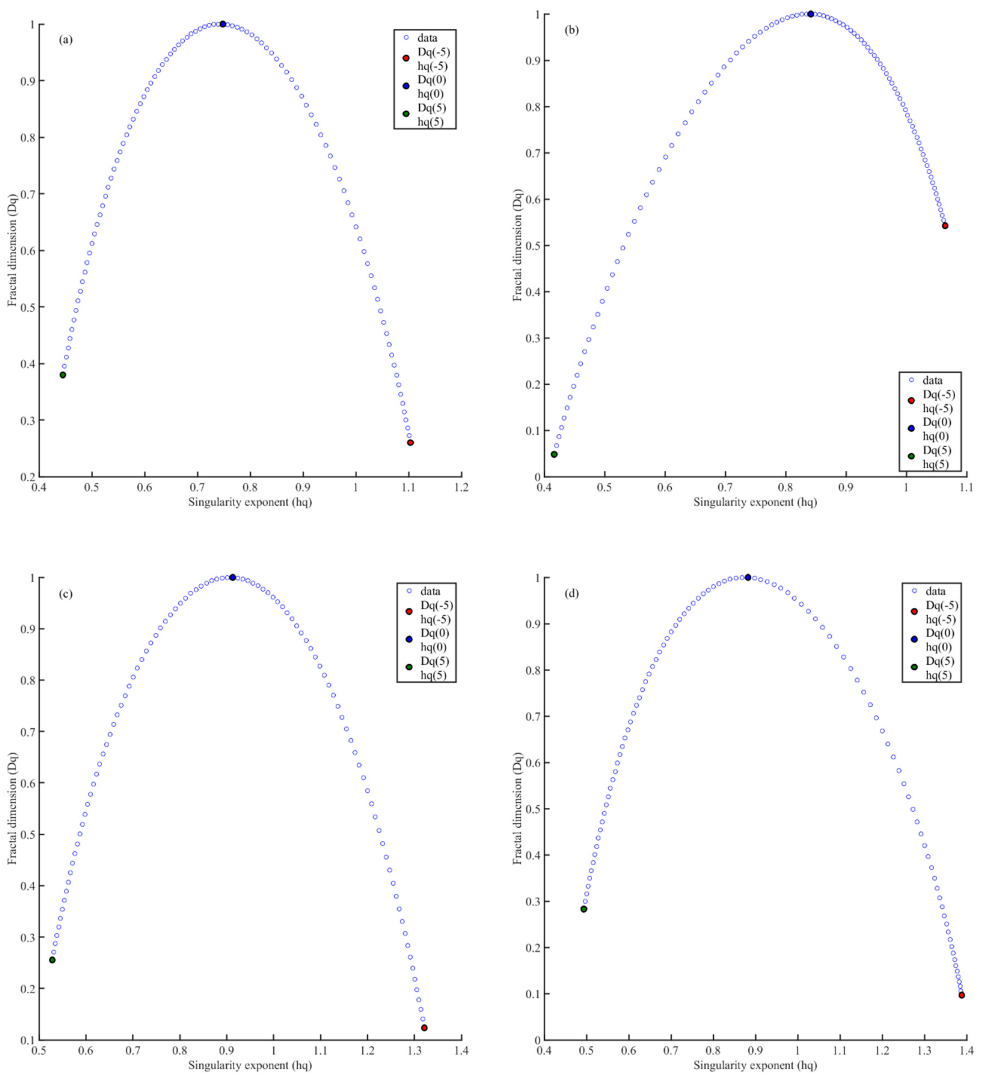
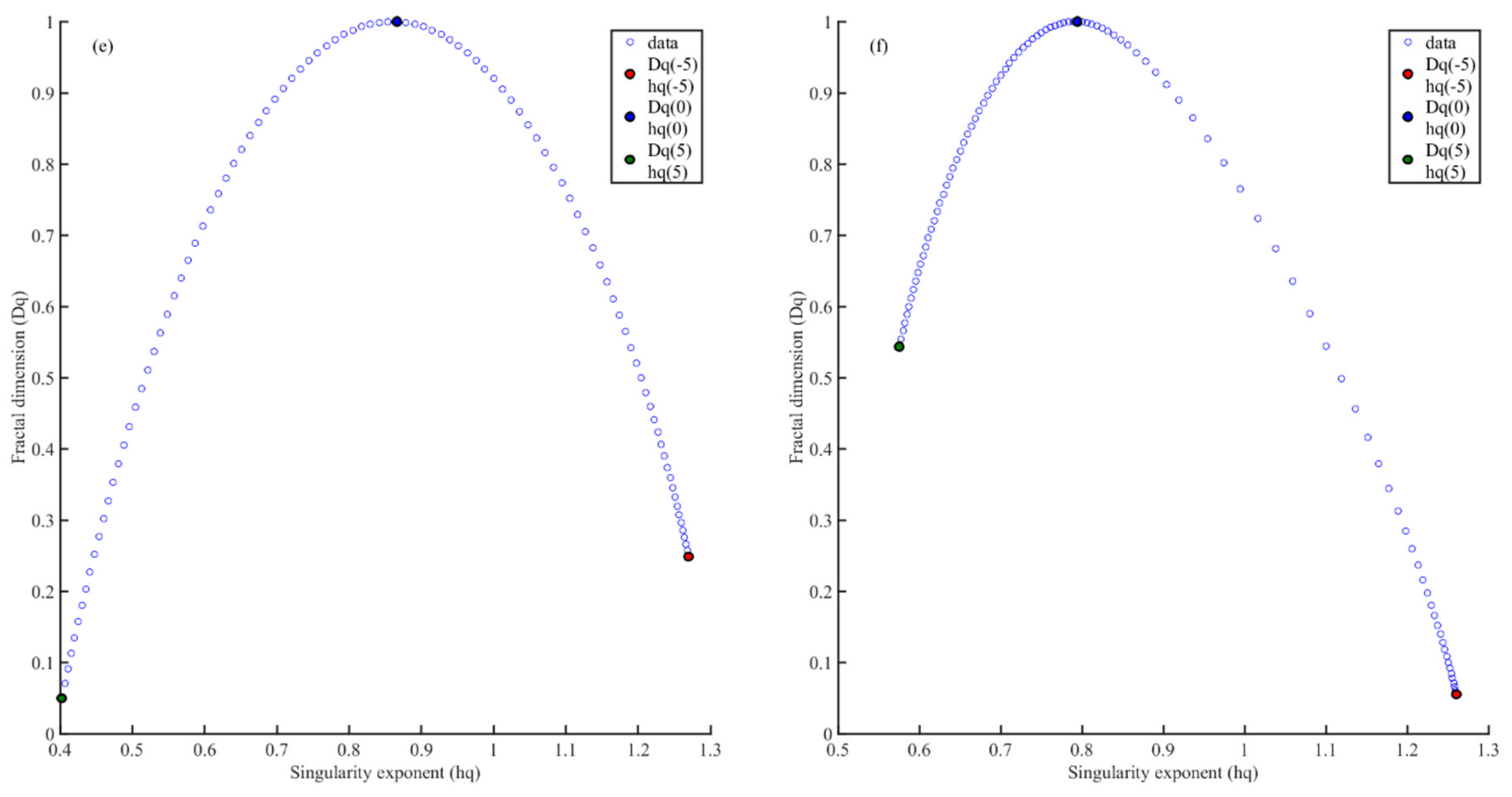
3.1. Multifractal Characteristics of the Profiles of Gully Shoulder Lines

Figure 3 shows the multifractal spectrum Dqhq relationship of the profiles of the gully shoulder lines in the six typical study sites, which were calculated using Equation (8). The figure also shows the singularity exponent hq and fractal dimension Dq. The singularity exponent hq of the q-order and its corresponding fractal dimension Dq here are the same as the parameters α and f(α) of the multifractal spectrum in related literature [23,24]. The spatial distribution and scaling properties of these variables have multifractal properties which can be described in term of a multifractal spectrum. This curve provides a synthesized picture of the full complexity of the scaling structure [25]. In addition, three parameters are very important to describe the complexity of the terrain profile. First, the width of the multifractal spectrum is Δhq. Second, the difference between the fractal dimensions of the maximum probability subset Dqmin and the minimum Dqmax. Third, the asymmetry of the curve. The width of the multifractal spectrum is Δhqhq = hqmaxhqmin). The higher the Δhq, the wider the probability distribution as well as, the larger the difference between the highest elevation and the lowest elevation, so the “richer” the terrain profile in structure. The range of the fluctuation order in this study is (−5, 5) because the multifractal spectrum is most sensitive to fluctuation orders in this range and insensitive outside this range [26]. According to Figure 3, all the multifractal spectral curves are bell-shaped within the fluctuation order (−5, 5), which indicates that the changes in the gully shoulder line profiles show multifractal characteristics at all six study sites. The wider the spectral width of the multifractal spectrum, the more complex the dataset structure is. Corresponding to different topographic profiles along the shoulder line in the study site, this means that the fluctuations of the topographic profile along the shoulder line are dramatic and complex. Sites with complicated topographic reliefs must have a fragmented surface, be densely distributed gullies, and have active gully erosion. If the width of the multifractal spectrum is smaller, it means that the structure of the dataset is smoother. It indicates that the topographic fluctuations along the shoulder line in this area are stable, the ground surface is relatively flat, the gully distribution is sparse, and the gully erosion activity is weak. The △hq parameter is the width of the multifractal spectrum and indicates the degree of multifractal strength. According to Table 1, the six study sites are arranged in the following order according to their multifractal characteristics, from strong to weak: Ganquan, Yijun, Yanchuan, Chunhua, Shenmu, and Suide. The stronger the multifractal degree, the more drastic the profile fluctuation of the gully shoulder line and the greater the variation in gully shoulder lines, indicating serious and active gully erosion in the loess gullies.
As can be seen from Figure 3d and Table 1, the top of the multifractal spectrum curve of the gully shoulder line at the Ganquan study site is relatively flat, and the multifractal spectrum width △hq is 0.8945, which is the largest among the six study sites; thus, the multifractal spectrum curve has a large distribution range. These characteristics show that the amplitude of the topographic fluctuation of the gully shoulder lines at Ganquan is relatively large and unevenly distributed. The difference between the fractal dimensions of the maximum probability subset (Dqmin) and the minimum one (Dqmax) is ΔDqDq = Dqmin − Dqmax). Dqmin and Dqmax reflect the number of the subset of the maximum and minimum probability, respectively. Thus, ΔDq < 0 represents that the chance of the terrain profile values lying at the lowest site is more than that at the highest site and vice versa. A right-skewed spectrum denotes the relatively strong dominance of high fractal exponents, corresponding to rough structures and a left-skewed spectrum indicate low ones (more smooth-looking). △Dq = −0.1864, which is less than 0, indicates that most profile sample points of gully shoulder lines are at wave troughs, further indicating that many gullies exist at this site and that gully erosion is severe. The topographic relief (fluctuations) along the shoulder line in the Ganquan sampling site has a very complex structure, and the topography is dominated by dramatic fluctuations with small magnitudes. In the topographic fluctuations along the shoulder line, the proportion of the terrain profile values is much lower at the peak than at the bottom. This further proves that the long ridge loess landform gully erosion intensity is the largest, gully erosion is the most active, there are many gullies, the gully density is large, and the size of the formed gully is also large. The Ganquan study site is located in the central and southern part of the Loess Plateau in northern Shaanxi, which is characterized by a large amount of rainfall, particularly in summer, and severe erosion of the loess ridge landform by water. The △hq value of the Yijun study site is 0.8674, second only to that at the Ganquan study site, and its gully shoulder line profile has strong fractal characteristics. Figure 3e shows that the multifractal spectrum curve of the Yijun study site has a longer left tail, which indicates a multifractal structure that is insensitive to local small topographic fluctuations △Dq = 0.1991, which is greater than 0, indicating that most of the sampling points of the gully shoulder lines are at wave peaks, with few loess gullies. Compared with the Ganquan sampling site, the topographic fluctuations along the shoulder line in the Yijun sampling site also have a complex structure, and the topographic fluctuations are also very strong. But the difference is that the topographic fluctuations of the Yijun sampling site are dominated by severe fluctuations with large magnitudes. In terrain relief profiles, the proportion at the peak is greater than at valleys. Because the Yijun sampling site is the loess fragmented tableland landform and is located in the southern part of the Loess Plateau, the annual precipitation is large, the rivers are numerous, and the gully erosion is active, but the gully erosion is basically in the head area of the ancient gullies.
Under the policy of returning farmland to forest land, vegetation restoration in the Loess Plateau is typically very good, whereas gully erosion is generally weak. The width of the multifractal spectrum at the Yanchuan study site is also large, with △hq = 0.7929 (Table 1), and the fractal characteristics of the gully shoulder line profile are also strong. △Dq = −0.1321, which is less than 0, and the sampling points of the gully shoulder lines are mostly at wave troughs, which indicates that gully erosion of the shoulder lines is active at the Yanchuan study site and there are many gullies. The multifractal curve is similar to that of the Ganquan study site (Figure 3c) and has the same structural characteristics. The fractal characteristics and gully erosion are slightly weaker than those of the Ganquan study site. The multifractal characteristics of the gully shoulder line profile in the Suide and Chunhua study sites are weak, with △hq values of 0.6479 and 0.6852, respectively, but the multifractal spectral structures of the two study sites are completely different. The multifractal spectrum at the Suide study site exhibits a right-sided structure, and the multifractal spectrum curve has a long left tail (Figure 3b), which indicate that the gully shoulder line profile has multifractal structure characteristics that are insensitive to local small (or gentle) topographic relief. The width of the multifractal spectrum of the terrain profile along the shoulder line in Suide sampling site is the smallest, and the structure of the topographic relief dataset is relatively smooth. The topography is mainly stable, which indicates that the topographic relief is gentle, and the peak data has a higher proportion of the profile data. It further shows that the gully density in this site is relatively small, the gully erosion is relatively low and inactive. Because the Suide sampling site is located in the northern part of the Loess Plateau with less rain and drought, the erosion intensity is less than that of the sediment, so a loess hill landform with smooth topographic relief has been formed. Conversely, the multifractal spectrum at the Chunhua study site has a left-sided structure, and the multifractal spectrum curve has a long right tail (Figure 3f), which indicate that the gully shoulder line profile has multifractal structural characteristics that are insensitive to local large (or severe) topographic fluctuations. The Chunhua sampling site with loess tableland landform has flat terrain without any fluctuation. Near the shoulder line, there are many gullies with relatively large depth and width. In this sampling site, gully erosion activity is relatively stable, and a few relatively active gully erosion sites caused by the transient runoff of heavy rain in summer. Comparing the study sites of Suide and Shenmu, gully erosion of shoulder lines at the Suide study site is more serious, and erosion of positive and negative topography is severe. Human activities (such as artificial terraces, warping dams, and other engineering measures) at the Suide study site have a greater impact on gully erosion. The Shenmu study site is a loess–aeolian and dune transition zone, with weak water erosion and wind erosion (Table 1). The multifractal spectrum parameter △hq = 0.6583, which indicates that the multifractal characteristics of the gully shoulder line profile are weak. The distribution of the multifractal spectrum curve is almost symmetrical, with no significant left or right deviation (Figure 3a), which shows that the number of sampling points along the gully shoulder line profile is equal to the number of peaks and gullies, and gully erosion of the shoulder lines is relatively weak.

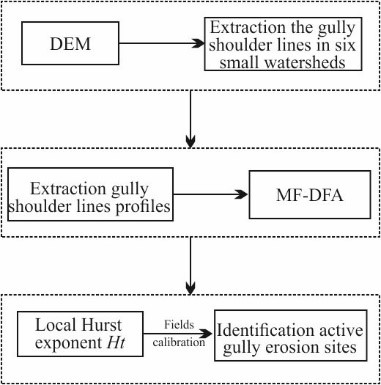
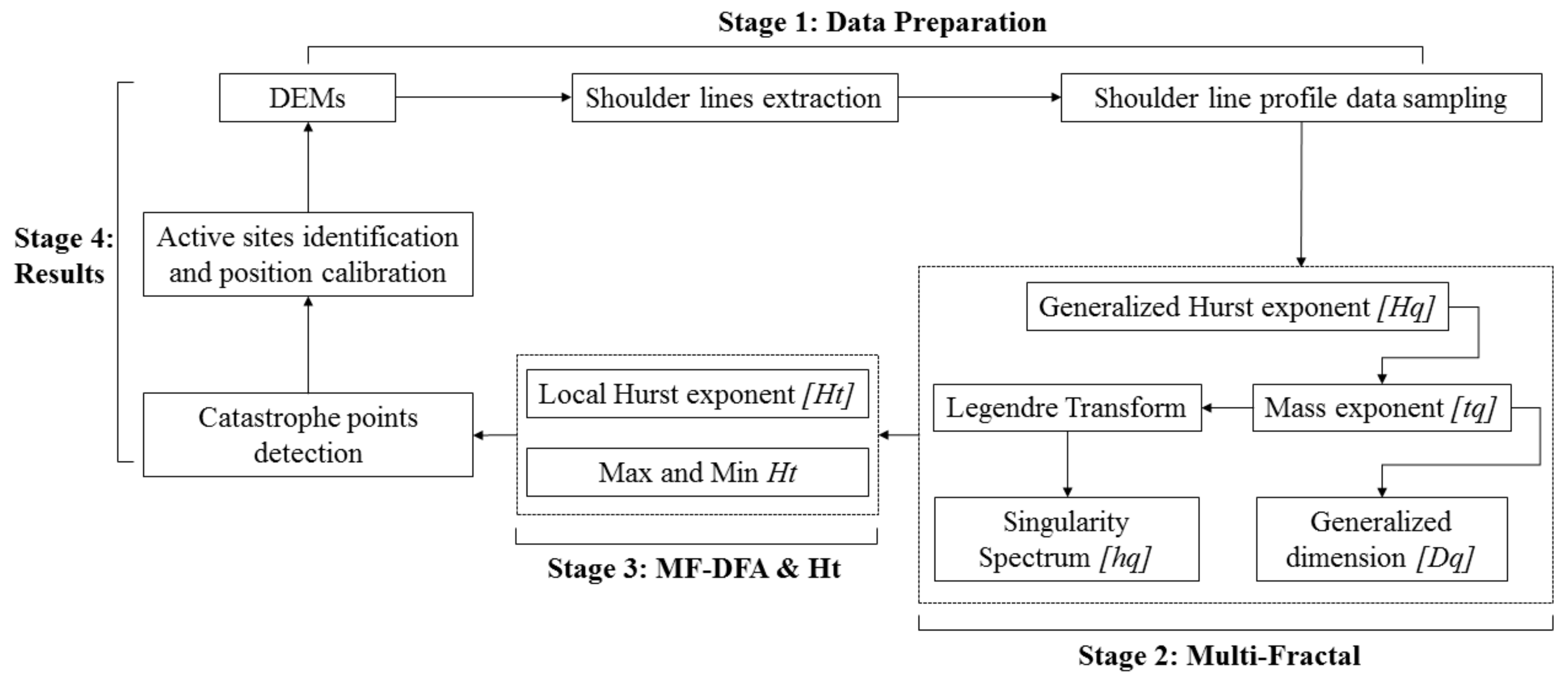
3.2. Identification of Points of Active Gully Erosion

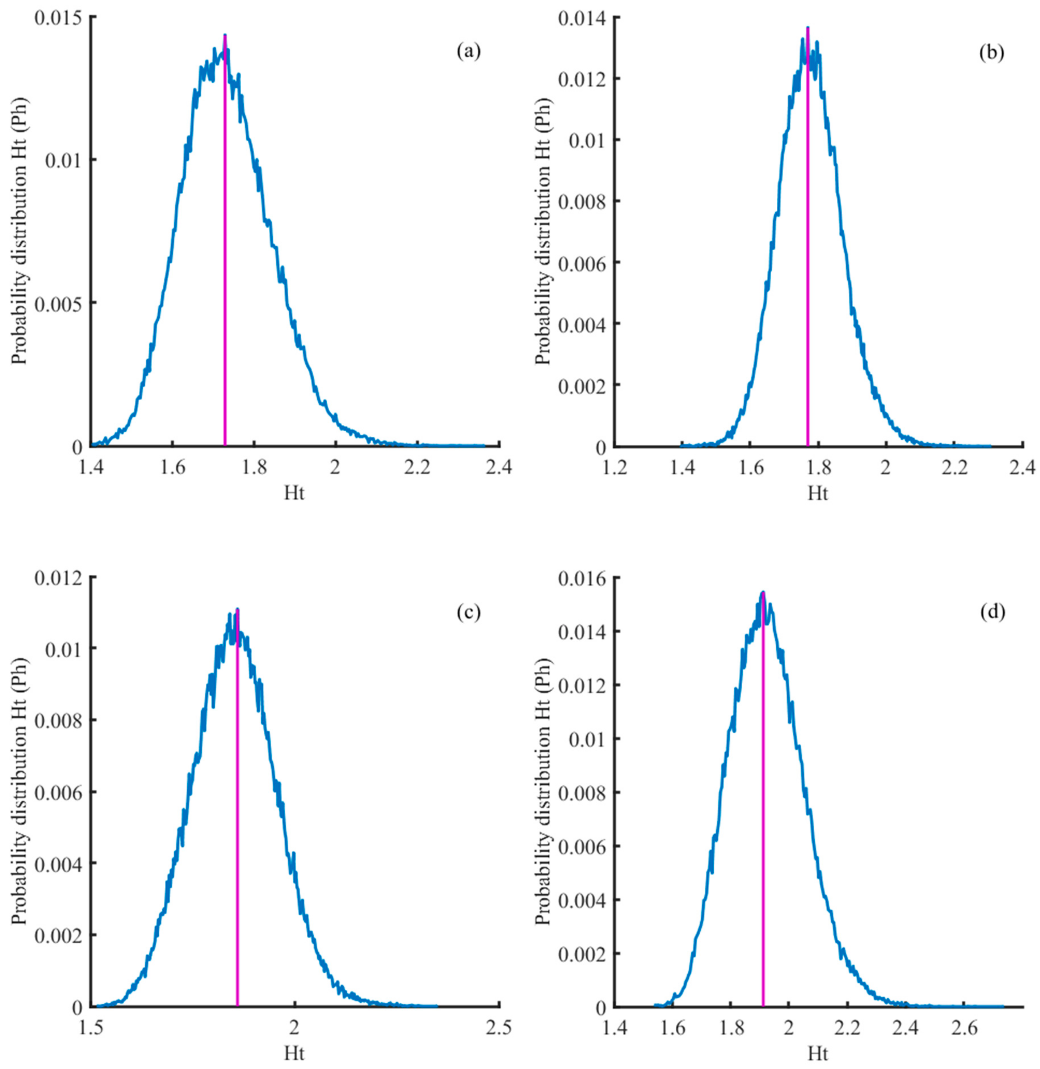
The relevant parameters of the multifractal spectrum can only measure the gully erosion intensity of the gully shoulder line profile at each study site from a global perspective; they cannot identify local sites of active gully erosion or specific regions for soil and water conservation. However, the local Hurst exponent (also called the time Hurst exponent, Ht), obtained using the multifractal generalized Hurst exponent, can solve this problem. The local Hurst exponent has an important feature when reflecting changes in the time series; it displays a mapping relationship between the position of the extreme point and the position corresponding to the original data series [23]. Due to the erosion effect of surface runoff, the main form of gully erosion in the loess small watershed is fluvial incision and headward erosion [27]. The active gully erosion sites are mainly located along the shoulder line that is the boundary between positive and negative terrain. Where gully erosion is active, the frequency of material and energy exchange is relatively high, and a large variety of gullies of different sizes and grades will be formed along the shoulder line. The topography of this part will show complex relief features, and the ground surface will become rugged and fragmented. The correspondence relationship between the min, max values of the local Hurst exponent of the profile data along the shoulder line, and the original topographic profile is able to identify such complex relief features. The original data sequence position corresponding to the point position where Ht reaches a maximum value must be the point at which the data do not fluctuate (data are stable), and the original data sequence corresponding to the point position where Ht reaches a minimum value must be the point at which the data fluctuate most substantially [26]. However, the local Hurst exponent obtained from the generalized Hurst exponent is affected by the analysis scale. That is, the overall average value of Ht will not change (only the extreme value will change), the maximum value will decrease with increasing analysis scale, and the minimum value will change irregularly with increasing analysis scale. In addition to these changes, the spatial positions of extreme points used to obtain their spatial distribution patterns will also change. In this study, a minimum analysis scale of 7 and a maximum analysis scale of 17 were selected to determine the effect of the analysis scale (Table 2).

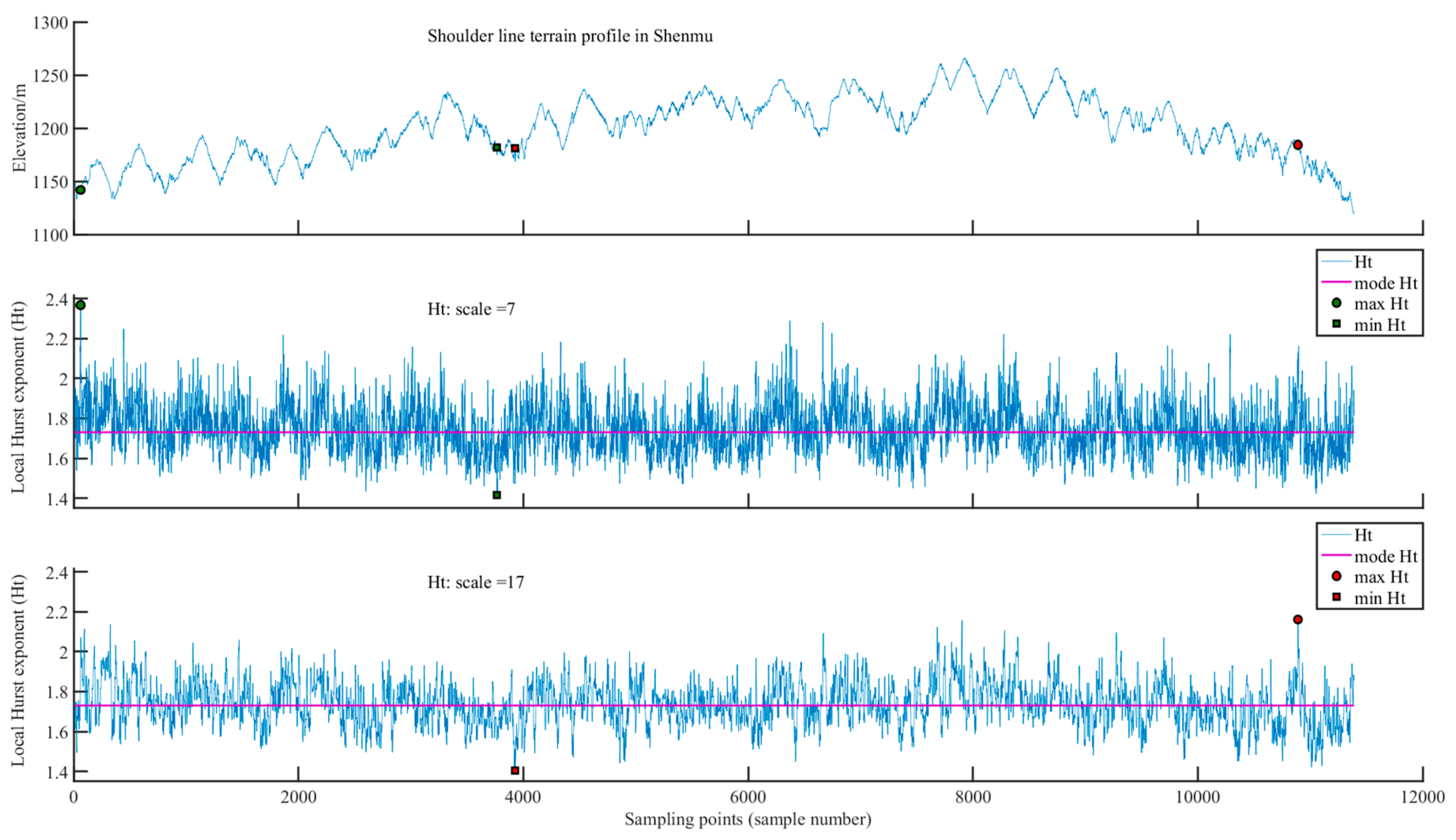
3.2.1. Shenmu Study Site

The average Ht of the section gully shoulder lines at the Shenmu study site is 1.7302 (Table 2). When the analysis scale is 7, the maximum Ht of the gully shoulder line profile is 2.3688, and the point is located near the water outlet of the catchment at the study site, at the 54th sample point. Here, topographic fluctuation of the gully shoulder line profile is stable (Figure 4), and gully erosion is not significant and relatively stable. The minimum Ht is 1.4171, located at the 3758th sample point, which indicates that the topography of the gully shoulder line profile changes sharply near this point, corresponding to active gully erosion. When the analysis scale is 17, the maximum Ht is 2.1617, located at the 10,884th sample point, which is also located near the water outlet of the basin, further indicating that the terrain in this area is gentle and that gully erosion is not active. The minimum Ht is 1.4026, located at the 3921st sample point, which is very close to the minimum value sample point for an analysis scale of 7. This shows that the topography of the gully shoulder line profile fluctuates substantially in this area. The gully shoulder line of the Shenmu study site is an area with active gully erosion from sample points 3758 to 3921; thus, soil and water conservation should be emphasized in this area. Gully erosion is relatively stable near the watershed outlet in the Shenmu sampling site, and gully erosion is more active at the head of the gully located in the middle of the watershed.

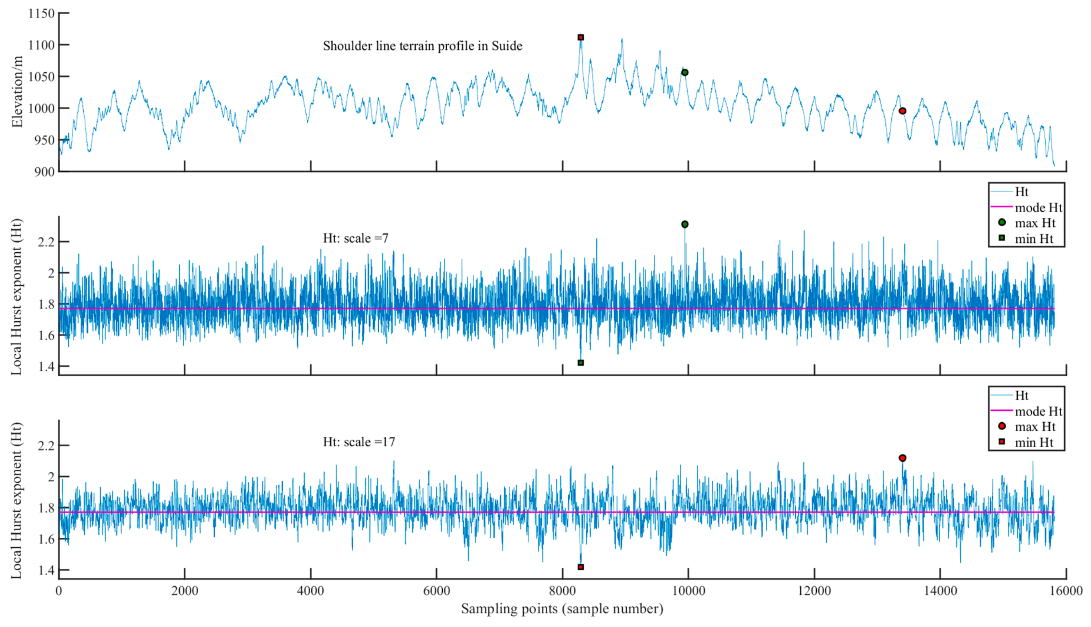
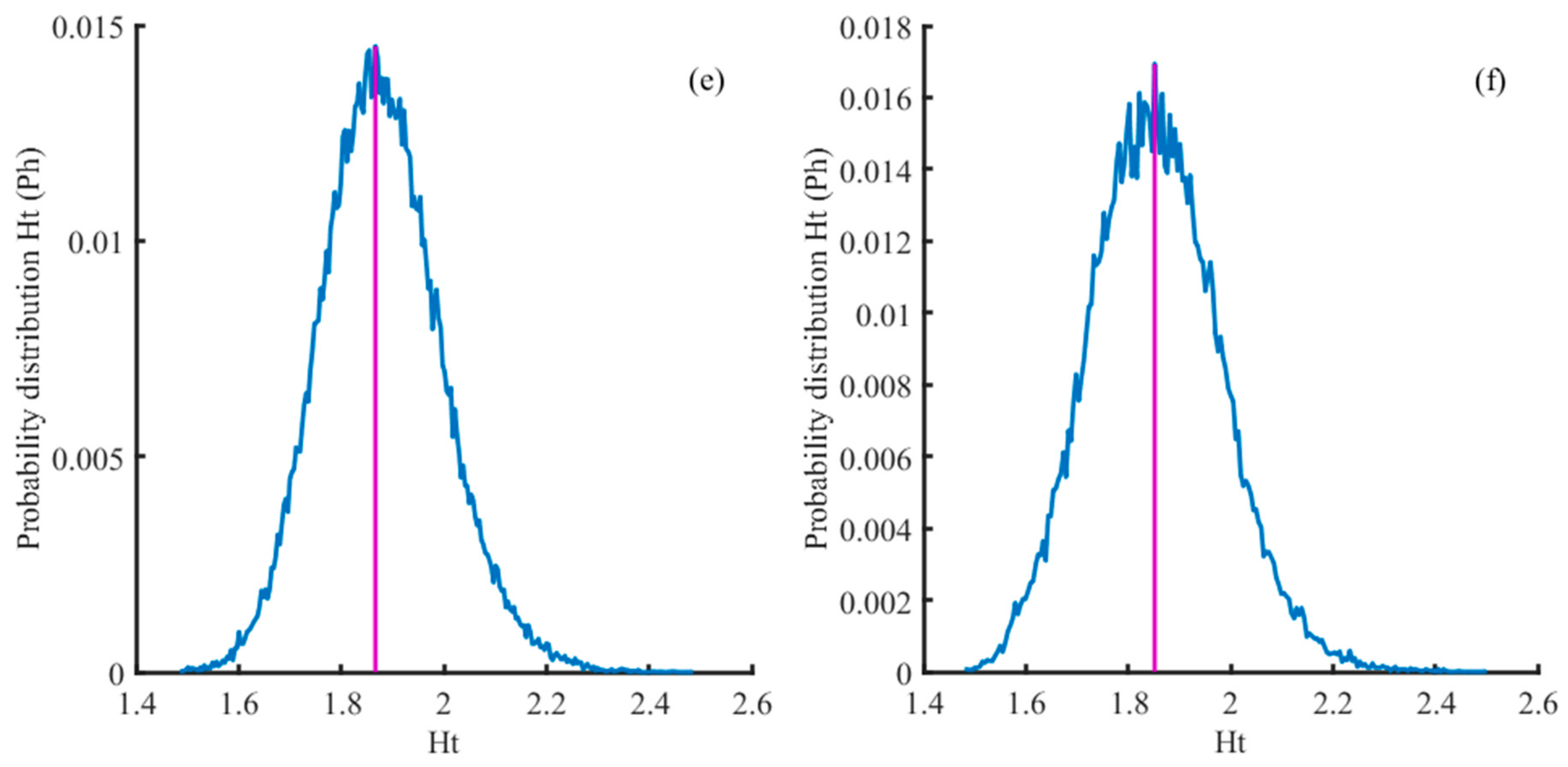
3.2.2. Suide Study Site

According to Figure 5, when the analysis scale is 7, the maximum Ht of the gully shoulder line profile at the Suide study site is 2.3106 (Table 2), located at the 9937th sample point, where the topographic change in gully shoulder lines is relatively small, which indicates that the terrain is gentle, gully erosion is not significant, and gully erosion activity is relatively stable. The minimum Ht is 1.4204, which corresponds to the 8284th sample point of the gully shoulder line profile. This suggests that the topography of the gully shoulder lines in this area varies substantially, landform erosion is serious, and gully development and erosion is severe. When the analysis scale is 17, the maximum Ht is 2.1184, located at the 13,397th sample point. The topographic fluctuation of the gully shoulder line at this site is relatively small, indicating that the terrain in the area is gentle and that gully erosion is not significant. However, the minimum Ht is 1.4160, located at the 8284th sample point, which is consistent with the location of the corresponding sample with an analysis scale of 7. This further indicates that the topography along the regional gully changes sharply and that gully development is relatively severe, representing the key area of active gully erosion at the Suide study site. The gully erosion active sites in the Suide sampling site are relatively concentrated, mainly distributed at the head of the gully in the upper reaches of the watershed, indicating that the gully is still growing.

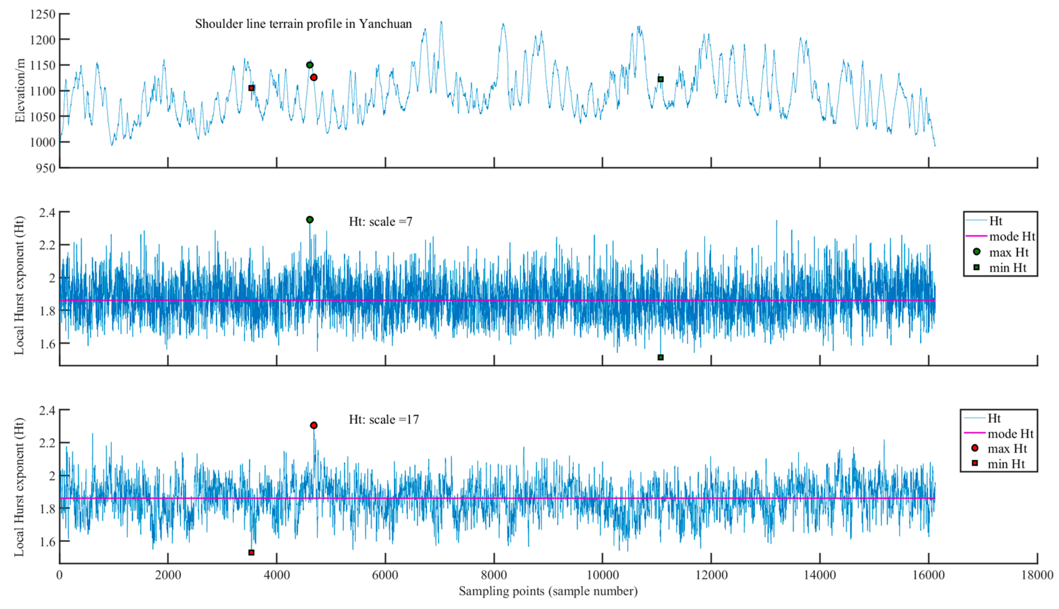
3.2.3. Yanchuan Study Site

For analysis scales of 7 and 17, the maximum Ht values are 2.3522 and 2.3048 (Table 2) and located at the 4603rd and 4676th sample points (Figure 6), respectively, indicating that the topography of the gully shoulder line in this area is less undulating, the terrain is gentle, and gully erosion is relatively stable. The positions of the sample points corresponding to the minimum Ht are quite different; the minimum Ht values for analysis scales of 7 and 17 are 1.5147 and 1.5292, corresponding to the 11,060th sample point and the 3529th sample point, respectively. This shows that there are many gully shoulder line profiles at the Yanchuan study site, where gully erosion is active. The topography of the gully shoulder lines in these two areas changes sharply, and gully erosion is severe and active. This is likely because the predominant landform in the Yanchuan study site is hills with loess and ridges and belongs to a temperate continental monsoon climate. The rainfall is lower and concentrated in summer rainstorms, which leads to active gully erosion and continuous development of gully heads. The distribution of gully erosion active sites in the Yanchuan sampling site is scattered, but it is also at the gully head position, while the distribution of gully erosion stable sites is concentrated.

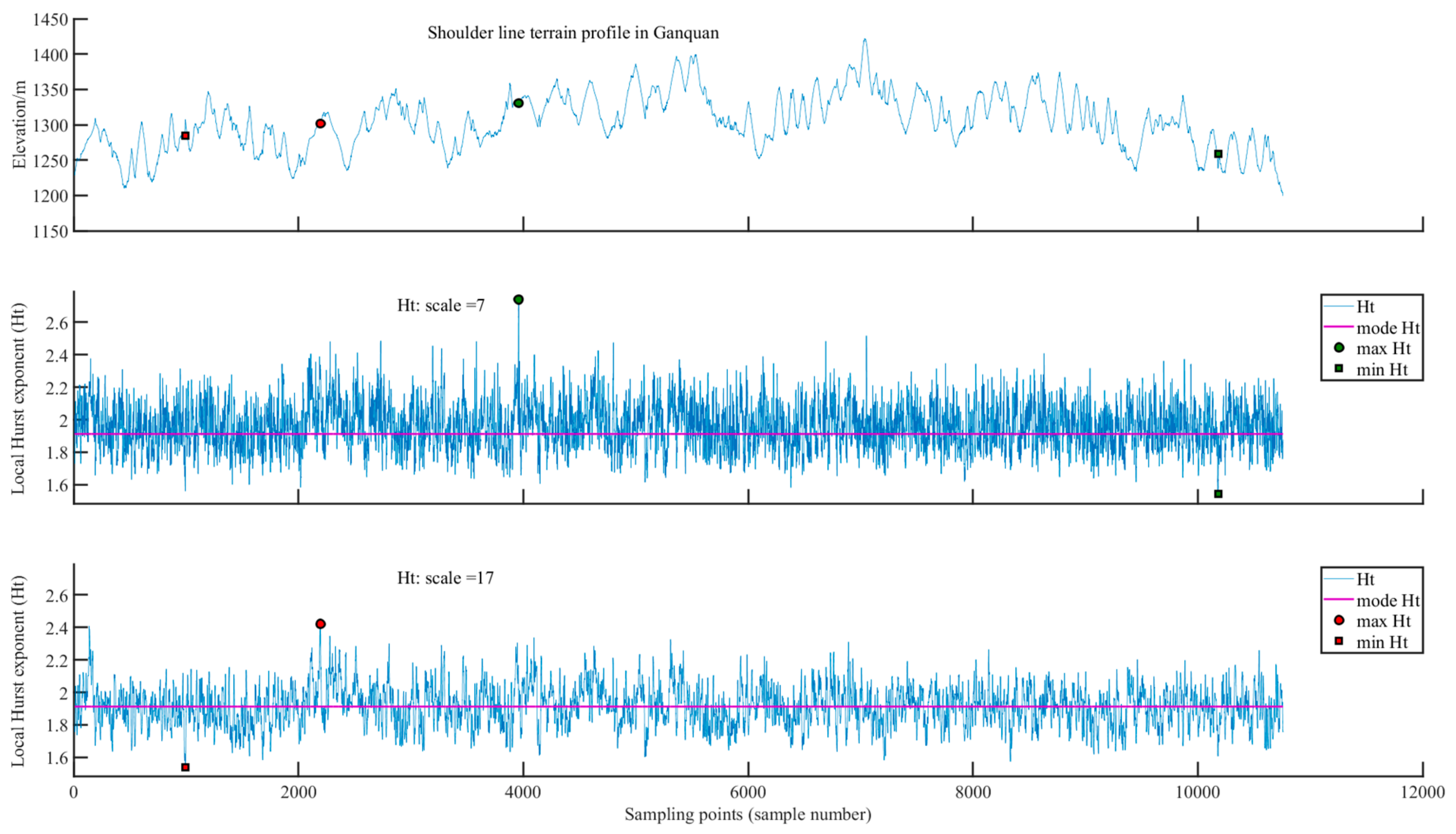
3.2.4. Ganquan Study Site

The extreme values of Ht for the gully shoulder line profiles at the Ganquan study site exhibit different sample point positions corresponding to the two analysis scales. When the analysis scales are 7 and 17, the maximum Ht values are 2.7400 and 2.4205 (Table 2), corresponding to the 3951st and 2188th sampling points, respectively (Figure 7). These points correspond to relatively small topographic fluctuations in the gully shoulder lines, which indicates gentle topography and relatively stable gully erosion. When the analysis scales are 7 and 17, the minimum Ht values are 1.5425 and 1.5367 (Table 2), corresponding to the 10,172nd and 986th sampling points, respectively (Figure 7). This indicates a sharp change in the regional topography of gully shoulder lines, serious soil erosion, and active gully development. These two regions are located on the north–south symmetrical slope not far from the water outlet of the river basin, which may have a low erosion benchmark. The landform type of the study site is ridge-shaped loess hills and gullies, characterized by surface erosion on the slope, sharp downcutting of gullies and rivers between the ridge and the ground, and active gully erosion. The distribution of gully erosion active and stable sites in the Ganquan sampling site is relatively concentrated, and the gully erosion active sites are mainly located near the outlet of the watershed, which indicates that the gully erosion in the Ganquan sampling site is developed and evolved by means of fluvial incision.

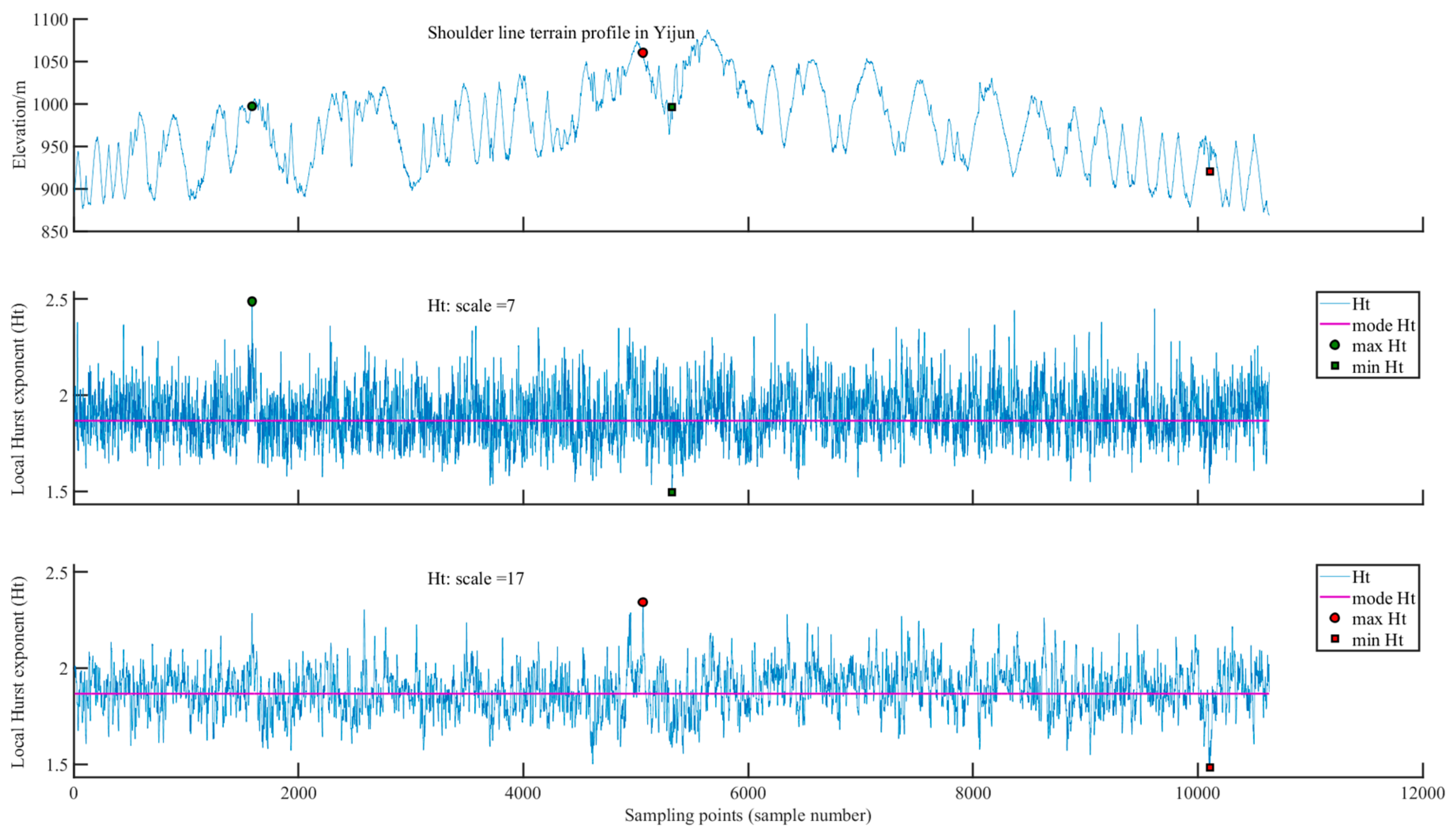
3.2.5. Yijun Study Site

The maximum Ht values for gully shoulder line profiles at the Yijun study site are 2.4881 and 2.3426 for analysis scales of 7 and 17 (Table 2), respectively. The corresponding sample points of gully shoulder lines are the 1580th and 5057th points (Figure 8), respectively. These maximum values correspond to small topographic fluctuations, gentle topography, and stable gully erosion. For analysis scales are 7 and 17, the minimum Ht values are 1.4962 and 1.4839 (Table 2), located at the 5316th and 10,101st sample points (Figure 8), respectively. The topography of the gully shoulder lines in the area near these two sample points varies greatly, which indicates that soil erosion is serious, and gully erosion is active. The area of stable gully erosion at an analysis scale of 17 and the area of active gully erosion at an analysis scale of 7 are spatially close but exhibit abrupt changes in gully erosion. The Yijun study site is predominantly loess gullies in long-ridge remnant tablelands, with substantial precipitation in the southern part of the Loess Plateau and gully erosion that is dominated by gravity erosion. The distribution of gully erosion active and stable sites in the Yijun sampling site is intertwined, which indicates that gully erosion activity in the loess fragmented landform is more complicated.

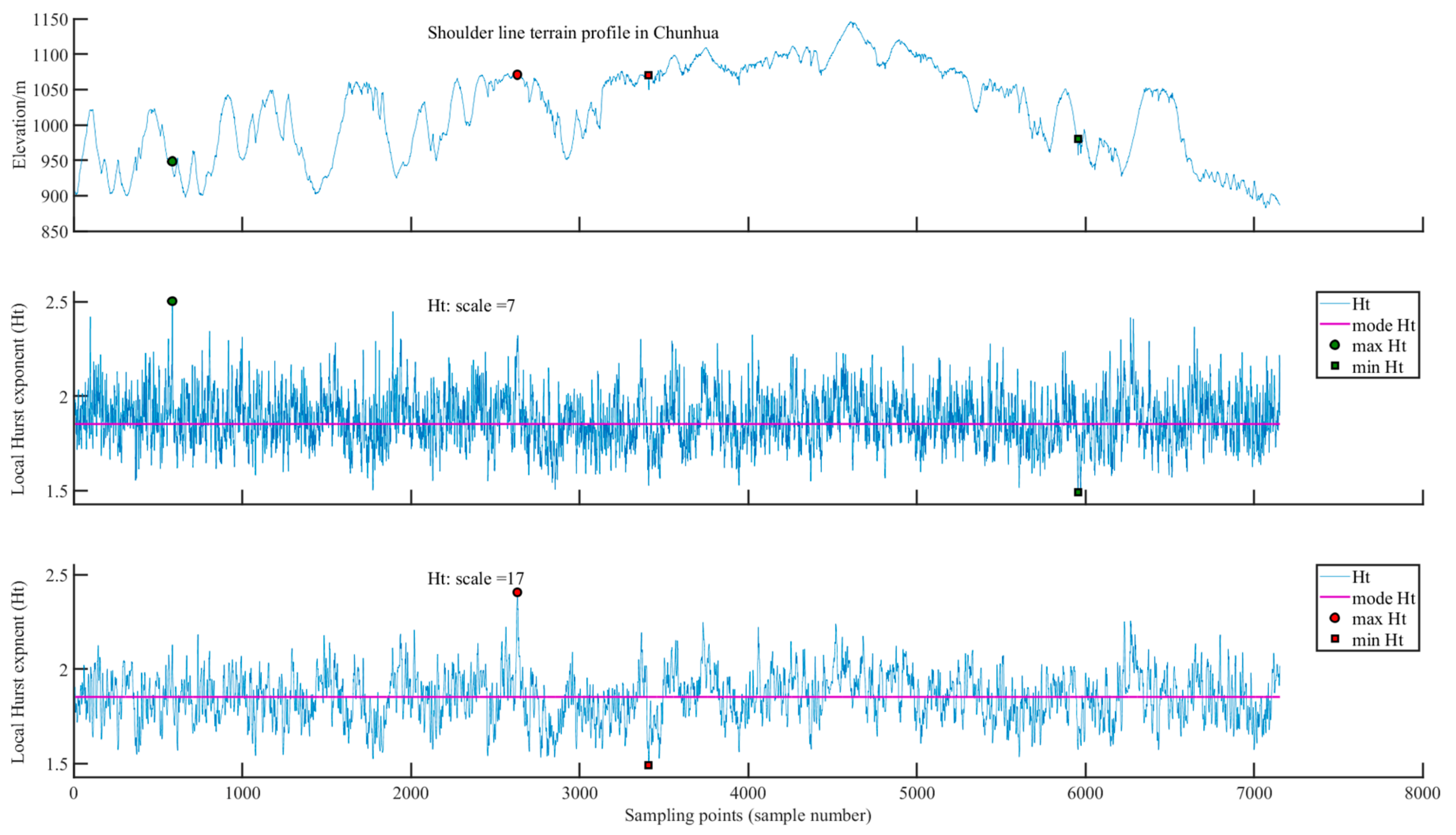
3.2.6. Chunhua Study Site

For analysis scales of 7 and 17, the maximum Ht values at the Chunhua study site are 2.5029 and 2.4065 (Table 2), corresponding to the 577th and 2624th sample points, respectively (Figure 9). These two sample points are located on the sunny slope of the watershed. The topographic changes in the gully shoulder lines are small, the vegetation coverage is good, soil erosion is not significant, and gully erosion is relatively stable. The minimum Ht values are 1.4896 and 1.4910 (Table 2), located at the 5948th and 3403rd sample points, respectively (Figure 9). These areas are located on the shady slope of the watershed, with sharp topographic fluctuations, severe soil erosion, and active gully development. The Chunhua study site is located in the southern part of the Loess Plateau. Annual precipitation is substantial and concentrated. The dominant landform type is loess tableland, and there is a large continuous tableland surface. The loess layer in the tableland area is thick, loose, and prone to collapse. Therefore, gravity erosion, hydraulic erosion, and headward erosion are severe. The surface of the tableland area is relatively complete, but the topography of the gully shoulder lines is relatively complex. The distribution of gully erosion active and stable sites in the Chunhua sampling site is also intertwined, which indicates that the gully erosion activity in the loess tableland landform is also complicated.

3.3. Calibration of Points of Active Gully Erosion

Based on the results of Ht analysis for the gully shoulder lines, active and stable points of gully erosion were calibrated for each study site. Figure 10a shows points of active gully erosion in the Shenmu sampling site, which are located at the head positions of larger sub-gullies, indicating that gully erosion is more active in this sub-gully and its size will further expand. Points of stable gully erosion are located near the watershed outlet, which reflects that the reference point of gully erosion in this site is stable, and that gully erosion in the main gully is relatively stable. This is predominantly because the dominant landform type in Shemu is loess–aeolian sand with little precipitation and inactive gully erosion. According to Figure 10b, points of active gully erosion in the Suide study site are located in the same position under different analysis scales, i.e., upstream of the gully head. Points of stable gully erosion are located on the northern bank of the gully. This shows that gully erosion in the Suide sampling site is generally active, and the gully is still developing. The distribution of active and stable gully erosion in the Yanchuan study site is more complicated; however, active erosion is again observed at the gully head positions of different size tributary gullies. A single point of stable gully erosion is located in one sub-gully (Figure 10c). Points of active gully erosion in the Ganquan sampling site are located at the gully head position of sub-gullies on the north and south sides near the watershed outlet. A point of stable gully erosion is located on the gully bank in the midstream of the watershed (Figure 10d). This indicates that gully erosion in the Ganquan sampling site is more active and predominantly due to vertical river cutting. Moreover, the erosion reference point is further reduced downstream. The spatial distribution of active and stable gully erosion in the Yijun and Chunhua study sites is similar (Figure 10e,f), with active erosion occurring at the gully heads of sub-gullies on both sides of the small watershed; however, stable gully erosion occurs near the watershed outlet.

4. Discussion

4.1. Analysis Scale of Local Root Mean Square (RMS)

In the analysis of the shoulder line profile based on MF-DFA, the selection of the analysis scale is very important as it is not only related to the data characteristics of the object itself but also to the statistical calculation. Points of active gully erosion can only be accurately identified by selecting the appropriate analysis scale; therefore, the analysis scale is crucial for identifying points of active gully erosion in different types of landform. To analyze the fluctuation trend of the shoulder line profile using the MF-DFA method, the root mean square (RMS) of the terrain profile data series is calculated. RMS is only sensitive to differences in the amplitude of variation and not to differences in the structure of the variation [26]. In psychology and medical signal research, the minimum segment sample size should be large enough to prevent errors in the computation of local fluctuation RMS [28]. A minimum segment size of at least 10 samples is typically considered for the computation of RMS [23].
The base data DEM used in this study has a resolution of 5 m, and sampling of the shoulder line profile data series is performed according to this resolution. When calculating the Ht data series of the shoulder line profile, if the analysis scale is too large, the calculation of local RMS will smooth out fluctuations with large magnitudes and exclude detailed information of the shoulder line profile. Moreover, Ht will exhibit smooth and slowly changing dynamics that are not well described by the probability distribution Ph [29]. However, if the analysis scale is too small, the sample is not large enough to calculate the local RMS, leading to errors during the calculation. Thus, an analysis scale range of [7,9,11,13,15,17] was used in this study, which provides a stable local RMS calculation for the shoulder line profile (Figure 11a–f).
In Figure 11, the regression line (purple center line) is the center of the spread of local RMS values in log-coordinates, and the blue dots represent the local RMS of shoulder line profiles for the six study sites. The local RMS values of the shoulder line profiles exhibit a stable and symmetric distribution between the maximum and minimum values for all study sites. When the analysis scale is 9, 11, 13, 15, and 17, the distribution of local RMS values is approximately similar with no major differences, except at Yanchuan (Figure 11c). However, when the analysis scale is 7, the local RMS values in all sampling sites exhibit a significantly larger distribution range, especially at Ganquan (Figure 11d). It is generally believed that the gully head experiences the most active gully erosion in the Loess Plateau, with the largest gully head development at the shoulder line. The size of the gully head is generally small; thus, the shoulder line profile data is sampled using the 5-m resolution DEM, an analysis scale of 7, and a spatial sampling distance of 35 m. This enables the detailed topographic relief of the shoulder lines to be expressed. If the analysis scale is 17, the sampling distance of the shoulder line profile is 85 m, which cannot effectively describe the detailed topographic fluctuations of the shoulder line profiles. Therefore, for a stable calculation analysis of the local RMS values of the shoulder line profile, an analysis scale of 7 is the most suitable.

4.2. Probability Distribution of the Local Hurst Exponent

The spatial variation of Ht in the shoulder line profile can be summarized in a histogram representing the probability distribution of Ht. Small Ht values in periods with large local fluctuations (i.e., large RMS) reflect the noise-like structure of the local fluctuations. In contrast, larger Ht values in periods with small local fluctuations (i.e., small RMS) reflect the random structure of the local fluctuations. The advantage of using Ht over the q-order Hurst exponent Hq is the ability of Ht to identify the time of structural changes within the shoulder line profile.
As shown in Figure 12a–f, the Ht values of six sampling sites exhibit a stable and symmetrical probability distribution centered on the mean Ht. This further reveals that the analysis scale used in the calculation of Ht to identify points of active gully erosion using shoulder line profile data series is suitable. The probability of maximum and minimum Ht values is small at all six sites and highest around the mean, with a deviation of 0.1. In addition to providing the distribution of extreme Ht values at each sampling site, the Ph curve of Ht can also measure the overall probability distribution of Ht at each sampling site. For example, for the Guanquan sampling site, the probability distribution curve has a maximum width of 1.1975 and a larger mean Ht than the other sampling sites (Figure 12d). The mean Ht decreases in the following order: Ganquan, Yijun, Yanchuan, Chunhua, Suide, and Shenmu. The probability distribution of Ht also reflects important structural features of the topographic relief of shoulder line profiles for different loess landforms.

4.3. Verification by Field Measurements

Due to the limitations of the fieldwork duration, cost, and convenience, the Suide study site was selected to validate the points of active and stable gully erosion. Field measurements were conducted in the summer of 2018. Figure 13b shows the sites of active gully erosion identified by the MF-DFA method in the Suide sampling site and their corresponding field locations. Due to active erosion, gullies of many different sizes appear along the shoulder line. Due to active headward erosion, a very wide gully was observed close to the boundary of the watershed (Figure 13c). Figure 13d shows three large-scale deep-cut gullies distributed in parallel along the shoulder line, which were formed by active runoff undercuts. At the point of active gully erosion, all gully erosion was an integrated erosion system. Below the shoulder line, landslides and debris slides were observed (Figure 13e). In comparison, the point of stable gully erosion was located on the bank of a tributary gully. Gully erosion here was relatively stable, gully bank expansion and the gully shoulder line remained stable, and no erosion of any scale was observed (Figure 13f). The main mode of gully erosion in the Loess Plateau was instantaneous surface runoff caused by heavy summer rains, especially in northern Shaanxi. This field verification work was conducted after heavy summer rainfall, which further ensured the validity of the gully erosion identification method proposed in this study.

5. Conclusions

In this study, topographic profile data of gully shoulder lines were obtained for six study sites representing the typical landform types of the Loess Plateau. The MF-DFA method was used to identify active gully erosion sites. The main conclusions are as follows:
1. Results demonstrate that MF-DFA is capable of detecting active gully erosion sites. Further work is necessary to understand the strengths and weaknesses of MF-DFA compared to existing methods
2. Differences were observed in gully shoulder line erosion activity and the spatial distribution of active gully erosion between the six study sites. According to the multifractal spectral parameter △hq (spectral width), the severity of gully erosion decreased in the following order according to landform type: loess ridge hill and gully region (Ganquan), loess long-ridge remnant tableland region (Yijun), loess ridge hill and gully region (Yanchuan), loess tableland region (Chunhua), loess hill and gully region (Suide), and loess–aeolian and dune transition region (Shenmu).
3. The local Hurst exponent was used to identify points of stable and active gully erosion at each study site. Active gully erosion was concentrated at the Shenmu and Suide study sites but more widely distributed at the other five study sites.
4. The results of the study sites of six typical landform types show that the active points are located at the head of the gully, and the stable points are located at the gully bank. It means that the layout and planning of soil and water conservation measures for gully erosion control should focus on the gully head where gully erosion is active.

Author Contributions

J.C. conceived, designed, and performed the experiments; J.C. and X.F. wrote the paper; Y.L. contributed to the data analysis; Y.Z. and J.L. made revisions; G.T. made revisions and supervised the study; W.W. provided critical feedback. All authors have read and agreed to the published version of the manuscript.

Funding

This research was funded by National Natural Science Foundation of China (No. 41930102, No. 41871313 and No. 41671389).

Acknowledgments

We are grateful to the members of DEM research group from Nanjing Normal University and the members of department of geographic information science in Nanjing Xiaozhuang University. We really appreciate the editors and anonymours reviewers for their meaningful comments for improving our manuscript.

Conflicts of Interest

The authors declare no conflict of interest.

References

  1. Hessel, R.; van Asch, T. Modelling gully erosion for a small catchment on the Chinese Loess Plateau. Catena 2003, 54, 131–146. [Google Scholar] [CrossRef]
  2. Stolte, J.; Liu, B.; Ritsema, C.J.; Van Den Elsen, H.G.M.; Hessel, R. Modelling water flow and sediment processes in a small gully system on the Loess Plateau in China. Catena 2003, 54, 117–130. [Google Scholar] [CrossRef]
  3. Valentin, C.; Poesen, J.; Li, Y. Gully erosion: Impacts, factors and control. Catena 2005, 63, 132–153. [Google Scholar] [CrossRef]
  4. Li, Z.; Zhang, Y.; Zhu, Q.; He, Y.; Yao, W. Assessment of bank gully development and vegetation coverage on the Chinese Loess Plateau. Geomorphology 2015, 228, 462–469. [Google Scholar] [CrossRef]
  5. Jing, K. A study on gully erosion on the Loess Plateau. Sci. Geogr. Sin. 1986, 6, 340–347. (in Chinese). [Google Scholar]
  6. Ariza-Villaverde, A.B.; Jiménez-Hornero, F.J.; De Ravé, E.G. Multifractal analysis applied to the study of the accuracy of DEM-based stream derivation. Geomorphology 2013, 197, 85–95. [Google Scholar] [CrossRef]
  7. Ariza-Villaverde, A.B.; Jiménez-Hornero, F.J.; De Ravé, E.G. Influence of DEM resolution on drainage network extraction: A multifractal analysis. Geomorphology 2015, 241, 243–254. [Google Scholar] [CrossRef]
  8. Roy, S.G.; Koons, P.O.; Osti, B.; Upton, P.; Tucker, G.E. Multi-scale characterization of topographic anisotropy. Comput. Geosci. 2016, 90, 102–116. [Google Scholar] [CrossRef] [Green Version]
  9. Dutta, S. Decoding the morphological differences between himalayan glacial and fluvial landscapes using multifractal analysis. Sci. Rep. 2017, 7, 1–8. [Google Scholar] [CrossRef] [Green Version]
  10. Wu, Y.; He, Y.; Wu, M.; Lu, C.; Gao, S.; Xu, Y. Multifractality and cross-correlation analysis of streamflow and sediment fluctuation at the apex of the Pearl River Delta. Sci. Rep. 2018, 8, 1–11. [Google Scholar] [CrossRef]
  11. Bai, Z.; Xu, Y.P.; Gu, H.; Pan, S. Joint multifractal spectrum analysis for characterizing the nonlinear relationship among hydrological variables. J. Hydrol. 2019, 576, 12–27. [Google Scholar] [CrossRef]
  12. Costabile, P.; Costanzo, C.; De Bartolo, S.; Gangi, F.; Macchione, F.; Tomasicchio, G.R. Hydraulic Characterization of River Networks Based on Flow Patterns Simulated by 2-D Shallow Water Modeling: Scaling Properties, Multifractal Interpretation, and Perspectives for Channel Heads Detection. Water Resour. Res. 2019, 55, 7717–7752. [Google Scholar] [CrossRef]
  13. Zhang, J.; Gupta, H.V.; Gao, G.; Fu, B.; Zhang, X.; Li, R. A Universal Multifractal Approach to Assessment of Spatiotemporal Extreme Precipitation over the Loess Plateau of China. Available online: https://www.hydrol-earth-syst-sci-discuss.net/hess-2019-430/ (accessed on 27 January 2020).
  14. Xu, M.; Li, Q.; Wilson, G. Degradation of soil physicochemical quality by ephemeral gully erosion on sloping cropland of the hilly Loess Plateau, China. Soil Tillage Res. 2016, 155, 9–18. [Google Scholar] [CrossRef]
  15. Wu, H.; Xu, X.; Zheng, F.; Qin, C.; He, X. Gully morphological characteristics in the loess hilly-gully region based on 3D laser scanning technique. Earth Surf. Process. Landf. 2018, 43, 1701–1710. [Google Scholar] [CrossRef]
  16. Capra, A. Ephemeral Gully and Gully Erosion in Cultivated Land: A Review. Drainage Basins and Catchment Management: Classification, Modelling and Environmental Assessment; Nova Science Publishers: Hauppauge, NY, USA, 2013. [Google Scholar]
  17. Zhu, T.X. Gully and tunnel erosion in the hilly Loess Plateau region, China. Geomorphology 2012, 153, 144–155. [Google Scholar] [CrossRef]
  18. Li, Y.; Poesen, J.; Yang, J.C.; Fu, B.; Zhang, J.H. Evaluating gully erosion using 137Cs and 210Pb/137Cs ratio in a reservoir catchment. Soil Tillage Res. 2003, 69, 107–115. [Google Scholar] [CrossRef]
  19. Wu, Y.; Cheng, H. Monitoring of gully erosion on the Loess Plateau of China using a global positioning system. Catena 2005, 63, 154–166. [Google Scholar] [CrossRef]
  20. Kantelhardt, J.W.; Zschiegner, S.A.; Koscielny-Bunde, E.; Havlin, S.; Bunde, A.; Stanley, H.E. Multifractal detrended fluctuation analysis of nonstationary time series. Phys. A: Stat. Mech. its Appl. 2002, 316, 87–114. [Google Scholar] [CrossRef] [Green Version]
  21. Xiong, L.Y.; Tang, G.A.; Li, F.Y.; Yuan, B.Y.; Lu, Z.C. Modeling the evolution of loess-covered landforms in the Loess Plateau of China using a DEM of underground bedrock surface. Geomorphology 2014, 209, 18–26. [Google Scholar] [CrossRef]
  22. Halsey, T.C.; Jensen, M.H.; Kadanoff, L.P.; Procaccia, I.; Shraiman, B.I. Fractal measures and their singularities: The characterization of strange sets. Phys. Rev. A 1986, 33, 1141. [Google Scholar] [CrossRef]
  23. Ihlen, E.A.F.; Vereijken, B. Interaction dominant dynamics in human cognition: Beyond 1/fα fluctuations. J. Exp. Psychol. Gen. 2010, 139, 436–463. [Google Scholar] [CrossRef] [PubMed]
  24. Xu, T.; Moore, I.D.; Gallant, J.C. Fractal, fractal dimensions and landscapes-a review. Geomorphology 1993, 8, 245–262. [Google Scholar] [CrossRef]
  25. Rodríguez-Iturbe, I.; Rinaldo, A. Fractal River Basins, Chance and Self-Organization; Cambridge University Press: New York, NY, USA, 1997. [Google Scholar]
  26. Ihlen, E.A.F. Introduction to multifractal detrended fluctuation analysis in Matlab. Front. Physiol. 2012, 3, 141. [Google Scholar] [CrossRef] [PubMed] [Green Version]
  27. Hu, Z.; Pan, B.; Guo, L.; Vandenberghe, J.; Liu, X.; Wang, J.; Fan, Y.; Mao, J.; Gao, H.; Hu, X. Rapid fluvial incision and headward erosion by the Yellow River along the Jinshaan gorge during the past 1.2 Ma as a result of tectonic extension. Quat. Sci. Rev. 2016, 133, 1–14. [Google Scholar] [CrossRef]
  28. Ihlen, E.A.; Vereijken, B. Multifractal formalisms of human behavior. Hum. Mov. Sci. 2013, 32, 633–651. [Google Scholar] [CrossRef] [PubMed]
  29. Cao, J.; Na, J.; Li, J.; Tang, G.; Fang, X.; Xiong, L. Topographic spatial variation analysis of loess shoulder lines in the Loess Plateau of China based on MF-DFA. ISPRS Int. J. Geo-Inf. 2017, 6, 141. [Google Scholar] [CrossRef]
Figure 1. Spatial distribution of the six sampling sites and gully shoulder lines: (a) location of the China in Asia, (b) location of the Shaanxi in China, (c) location map of the sampling sites, (d) Chunhua, (e) Yijun, (f) Ganquan, (g) Yanchuan, (h) Suide, and (i) Shenmu. Shoulder lines are shown in red.
Remotesensing 12 00589 g001
Figure 2. Workflow of the whole process method in this study.
Remotesensing 12 00589 g002
Figure 3. Multifractal spectrum of gully shoulder lines at the six study sites: (a) Shenmu, (b) Suide, (c) Yanchuan, (d) Ganquan, (e) Yijun, and (f) Chunhua.
Remotesensing 12 00589 g003aRemotesensing 12 00589 g003b
Figure 4. Local Hurst exponents of shoulder line profiles at the Shenmu sampling site for different analysis scales.
Remotesensing 12 00589 g004
Figure 5. Local Hurst exponents of shoulder line profiles at the Suide site for different analysis scales.
Remotesensing 12 00589 g005
Figure 6. Local Hurst exponents of shoulder line profiles at the Yanchuan site for different analysis scales.
Remotesensing 12 00589 g006
Figure 7. Local Hurst exponents of shoulder line profiles at the Ganquan site for different analysis scales.
Remotesensing 12 00589 g007
Figure 8. Local Hurst exponents of shoulder line profiles at the Yijun sampling site for different analysis scales.
Remotesensing 12 00589 g008
Figure 9. Local Hurst exponents of shoulder line profiles at the Chunhua sampling site for different analysis scales.
Remotesensing 12 00589 g009
Figure 10. Calibration of points of active and stable gully erosion derived from Ht values of gully shoulder lines from corresponding DEM data for six sampling sites. Blue points represent stable points, and yellow points represent active points. (a) Shenmu, (b) Suide, (c) Yanchuan, (d) Ganquan, (e) Yijun, and (f) Chunhua.
Remotesensing 12 00589 g010
Figure 11. Local root mean square (RMS) values for different analysis scales at the six sampling sites: (a) Shenmu, (b) Suide, (c) Yanchuan, (d) Ganquan, (e) Yijun, and (f) Chunhua.
Remotesensing 12 00589 g011aRemotesensing 12 00589 g011b
Figure 12. Probability distribution of the local Hurst exponent (Ht) of shoulder line profiles for the six sampling sites: (a) Shenmu, (b) Suide, (c) Yanchuan, (d) Ganquan, (e) Yijun, and (f) Chunhua.
Remotesensing 12 00589 g012aRemotesensing 12 00589 g012b
Figure 13. Field analysis at the Suide sampling site used to validate the calculated sites of active and stable gully erosion: (a) Suide study site, (b) general overview of points of active gully erosion in Suide, (ce) detail of points of active gully erosion, and (f) general overview of points of stable gully erosion.
Remotesensing 12 00589 g013
Table 1. Parameters of the shoulder line multifractal spectra at the six study sites.
Study SitesFluctuation Order qFractal Dimension DqSingularity Exponent hqDqhq
Shenmu−50.25991.1036−0.11980.6583
010.7395
50.37970.4453
Suide−50.54231.06450.49410.6479
010.8344
50.04820.4166
Yanchuan−50.12331.3213−0.13210.7929
010.9016
50.25540.5284
Ganquan−50.09651.3885−0.18640.8945
010.8683
50.28290.4940
Yijun−50.24851.26970.19910.8674
010.8540
50.04940.4023
Chunhua−50.05491.2607−0.48820.6852
010.7890
50.54310.5755
Table 2. Parameters of local Hurst exponents of shoulder line profiles in the six sampling sites.
Study SitesAnalytical ScaleHt MeanHt MaximumHt Minimum
Shenmu71.73022.36881.4171
172.16171.4026
Suide71.77012.31061.4204
172.11841.4160
Yanchuan71.86072.35221.5147
172.30481.5292
Ganquan71.91222.74001.5425
172.42051.5367
Yijun71.86692.48811.4962
172.34261.4839
Chunhua71.85182.50291.4896
172.40651.4910

