Technical Note

Automatic Mapping of Center Pivot Irrigation Systems from Satellite Images Using Deep Learning

1
Agrosatélite Applied Geotechnology, Florianópolis SC 88050-000, Brazil
2
Imazon—Instituto do Homem e Meio Ambiente da Amazônia, Belém PA 66055-200, Brazil
*
Author to whom correspondence should be addressed.
Remote Sens. 2020, 12(3), 558; https://doi.org/10.3390/rs12030558
Submission received: 13 December 2019 / Revised: 31 January 2020 / Accepted: 3 February 2020 / Published: 7 February 2020
(This article belongs to the Special Issue Deep Learning and Remote Sensing for Agriculture)

Abstract

:
The availability of freshwater is becoming a global concern. Because agricultural consumption has been increasing steadily, the mapping of irrigated areas is key for supporting the monitoring of land use and better management of available water resources. In this paper, we propose a method to automatically detect and map center pivot irrigation systems using U-Net, an image segmentation convolutional neural network architecture, applied to a constellation of PlanetScope images from the Cerrado biome of Brazil. Our objective is to provide a fast and accurate alternative to map center pivot irrigation systems with very high spatial and temporal resolution imagery. We implemented a modified U-Net architecture using the TensorFlow library and trained it on the Google cloud platform with a dataset built from more than 42,000 very high spatial resolution PlanetScope images acquired between August 2017 and November 2018. The U-Net implementation achieved a precision of 99% and a recall of 88% to detect and map center pivot irrigation systems in our study area. This method, proposed to detect and map center pivot irrigation systems, has the potential to be scaled to larger areas and improve the monitoring of freshwater use by agricultural activities.

Graphical Abstract

1. Introduction

In some regions, factors such as climate change, agricultural expansion, population growth, and increasing urbanization have caused an increase in the demand for water, leading to imbalances in supply and demand, and consequently, water shortages. Irrigated agriculture is one of the main sources of water demand, accounting for over 70% of the water withdrawal in the world [1]. The Food and Agriculture Organization of the United Nations (FAO) estimates that an area of more than 324 million hectares is equipped with irrigation infrastructure in the world, and 85% of it is actually irrigated [2].
The increasing use of water for agricultural irrigation can also cause problems on a regional scale. In some arid and semi-arid regions of India, the increase of irrigated agriculture intensified the process of soil salinization and waterlogging due to intensive seepage into the ground water, resulting in declining biodiversity and other environmental problems in agro-ecosystems [3]. In the Tarim River basin, in China, the intensive exploitation of water resources has caused severe conflicts among water users and serious environmental problems [4], such as the drying up of the downstream 321 km of the river and its terminal lakes, and a great reduction in ground water level [5]. In the Heihe River basin, in China, the rapidly increasing demands for agricultural water in recent decades, among other factors, have led to water shortages that are restricting the sustainable development of the region [6].
With an area of 6.9 million hectares of irrigated agriculture [7], Brazil is among the 10 countries in the world with the largest areas equipped with irrigation infrastructure [2]. Center pivot irrigation systems are some of the most common irrigation methods in the country, representing and area of 1.4 million ha. According to the National Water Agency of Brazil (ANA) [8], there has been a strong and persistent growth of center pivot irrigated agriculture in recent decades, which accelerated further after 2010. In 1985, 363 pivot points, irrigating an area of 31,000 ha, were identified. In 2000, 490,500 ha were already equipped for irrigation at 6680 points. In 2017, the area tripled to 1,476,000 hectares at 23,181 points. The current area is 47 times larger than the area mapped in 1985. The Atlantic Forest and Cerrado concentrate, respectively, have 11.5% and 78.0% of their total areas irrigated by center pivot systems. Caatinga, Pampa, and Amazon account for 4.7%, 4.2%, and 1.6%, respectively [8]. The concentration in the Cerrado occurs as a result of the expansion of agriculture to areas with greater water deficit and the suitability of these systems for large areas with relatively flat ground and the predominant soil types in the region.
As the use center pivot irrigation systems is a growing trend, their accurate mapping is important for supporting a better management of available water resources. Center pivot irrigation systems form large circular patterns that can be easily seen from satellite images. Thanks to this, remote sensing has been widely used in the identification of areas irrigated by center pivot systems. In the 80s, Carlson et al. [9] described the use of Landsat 5 TM Band-3 images to monitor center pivot irrigation systems in the U.S. state of Nebraska from 1972 to 1986, identifying a growth from 2665 pivots in 1972 to 26,208 in 1986, a nearly ten-fold increase over 14 years. In Brazil, the National Water Agency of Brazil (ANA) [8] used images from medium spatial resolution satellites to perform a historical mapping of center pivot irrigation systems for different years, as far back as 1985.
These works show that satellite images are adequate for the remote identification of center pivot irrigation systems. However, both are based on the visual interpretation of the images by human specialists. While this process is reliable and generally produces accurate results, it is also expensive and time-consuming. The use of automatic mapping systems could reduce costs and allow for the mapping of large areas in a much shorter period. Methods based on the Hough Transform [10] can be used to detect the circular patterns of center pivot irrigation systems. However, such methods would be unable to differentiate center pivot irrigation systems from other circular structures. Boundary shape-based methods also are not robust for partially cultivated pivots, which have forms like semicircles or quarter circles, and have irregularities in the edges of the circular fields [11]. Yan and Roy [11] present a method for the automated segmentation of crop fields from multi-temporal web-enabled Landsat data, achieving an overall pixel level accuracy of 90.1% in the test set. Their method, however, does not differentiate crops irrigated by center pivot systems from those cultivated with other irrigation methods or not irrigated at all. It also relies on manually determined parameters that may change depending on the region.
Zhang et al. [12] presented an approach based on image classification convolutional neural networks to automatically detect center pivot irrigation systems. The authors experimented with three different architectures: LeNet-5 [13], AlexNet [14], and VGGNet [15]. The classifiers were trained on Landsat 5 TM images from the U.S. state of Colorado. Their approach, however, has some limitations that make it inadequate for areas where there is a great variation among the radii of pivots, such as in Brazil. Another limitation of their method is that its only output is the position of the center of the pivot. It does not account for partially cultivated or irregularly shaped pivots, and this could lead to errors in the estimation of the irrigated area in some regions.
In this study, we present a novel approach for the automatic detection and the mapping of the location, shape, and area of center pivot irrigation systems. Our objective is to propose a fully automated method that is faster, more accurate, and more scalable in comparison to mapping by visual inspection. The method must also be suitable to detect and map the center pivots of different shapes and sizes and under different vegetative stages.

2. Materials and Methods

2.1. Study Area

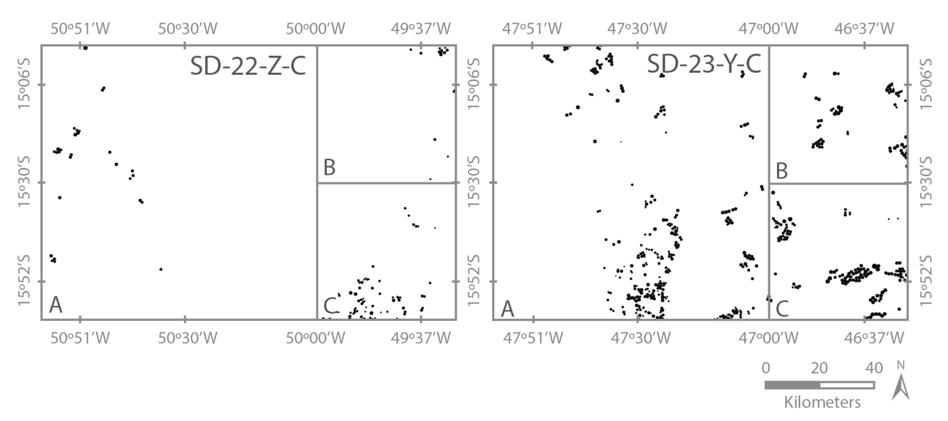
The study area is located between the states of Goiás (GO) and Minas Gerais (MG), in Brazil; more specifically, in the areas covered by grids SD-23-Y-C and SD-22-Z-C (Figure 1) of the Brazilian Continuous Cartographic Base at scale 1:250,000. Both grids are in the Cerrado biome. Each grid covers an area of 1.8 Mha, resulting in a total area close to 3.7 Mha. Goiás is the state with the second largest center pivot irrigated area (272,330 ha) in Brazil (18.4% of the total area irrigated by center pivot systems in Brazil) [8]. In 2017, the SD-23-Y-C grid had 37,285 ha, and the SD-22-Z-C grid had 7357 ha irrigated by center pivot systems, totaling 44,642 ha in both grids of the study area [8].

2.2. Image Dataset

2.2.1. Planet Images

In this study, we used a total of 42,731 Analytic PlanetScope Ortho Scenes with a radiometric resolution of 12 bits and four spectral bands with resolutions of 455–515 nm (Blue), 500–590 nm (Green), 590–670 nm (Red), and 780–860 nm (NIR), each covering an average area of 22,500 ha. We used images of the grid areas from the period of August 2017 to November 2018. These images were acquired by PlanetScope satellites in two orbits: (i) the International Space Station orbit, with an altitude of 400 km (spatial resolution of 3 m per pixel) at an inclination of 51.6 degrees to Earth’s equator, and (ii) heliosynchronous orbit with an altitude of 475 km (spatial resolution of 3.7 m per pixel) with a nearly polar inclination of 98 degrees [16].

2.2.2. Planet Mosaics

Each PlanetScope image tile comes with an unusable data mask (UDM). The UDM offers some indication of pixels with cloud and shadow, but it has low level of precision when detecting those targets, as assessed by our research team via visual inspection. A single PlanetScope image also covers a relatively small area and oftentimes has a tilt angle that adds many nodata pixels at the borders of the image. These factors, among others, make the extraction of noise-free samples from a single PlanetScope image a difficult task. To overcome this problem and generate a dataset free of noise, such as clouds and shadows, we used median mosaics. Initially, all the images were converted from radiance to top-of-atmosphere (TOA) reflectance. From the TOA reflectance images, two mosaics were built, one for each of the selected grids, using the median of the images with cloud cover below 1%. The information about the amount of cloud cover was extracted from the PlanetScope image metadata. All the images from the period of August 2017 to November 2018 in the collection were used in the creation of the median image mosaics. To create a median mosaic, the values of all the images for each band of each pixel are ordered, and the medians of such values are selected as the values of each pixel in each band. This means that a single pixel of the median mosaic may be composed of pixels of several different images, but each band has the value of that exact pixel in a single image. This allowed us to create a cloud-free mosaic to be used in the detection and extraction of center pivot irrigation systems and also helped us to reduce atmospheric noise and to normalize the spectral information across the image tile. Because the cloud pixels tend to have the highest values in the image and shadow pixels tend to have the lowest values, this makes the median of all values a cloud and shadow-free pixel value. Beyond the median, we did not use any atmospheric or radiometric correction techniques. In convolutional neural networks, maintaining noise in the data or even adding artificial noise can contribute to a better generalization of the model, decrease overfitting, and reduce the training loss [17,18]. Our mosaics were generated using the Google Earth Engine [19], a cloud-based geospatial processing platform.

2.2.3. Training Data

Finally, center pivot irrigation systems present in the mosaic images were annotated by a specialist through visual inspection.
We divided each of the two images in our dataset into three regions: one for training, covering two-thirds of each image; one for validation, which covers one-sixth of each image; and one for testing, also covering one-sixth of each image, following the protocol proposed by Hastie et al. [20]. The division was performed as shown in Figure 2. We chose to use different regions for training, validation, and testing, to prevent overlapping patches generated in the data augmentation process (see Section 2.4) from being assigned to different sets, as this could lead to the model overfitting to the validation and training sets.

2.3. Network Architecture

We used U-Net [21], a convolutional neural network (CNN) architecture developed for biomedical image segmentation. U-Net has achieved state-of-the-art results on the ISBI EM segmentation challenge [22] and the ISBI cell tracking challenge [23]. The U-Net has also been successfully employed in remote sensing applications, such as the detection of features [24], the extraction of water bodies from satellite imagery [25], and the extraction of buildings from aerial imagery [26].
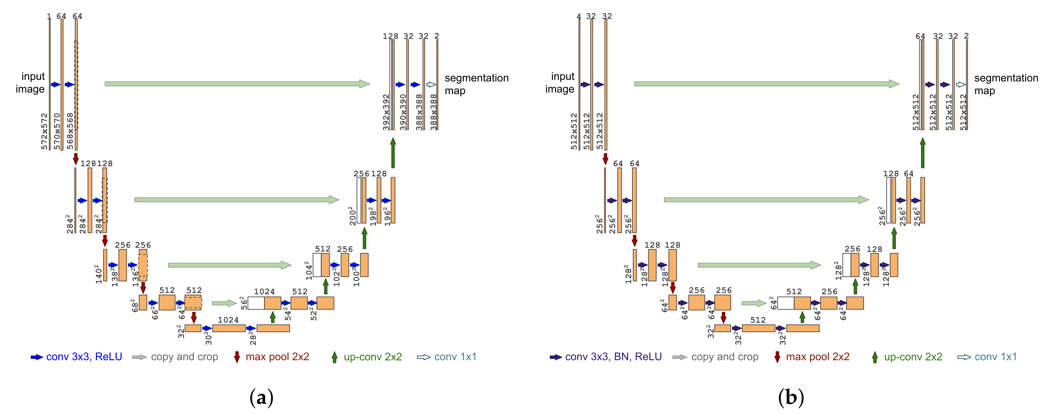
The U-Net architecture is illustrated in Figure 3a. It consists of a contracting path (left side) and an expansive path (right side). The contracting path follows the typical architecture of a deep convolutional network [14,15]. It is composed of successive convolutional (unpadded convolutions), ReLU, and max pooling layers that downsample the input while increasing the number of feature channels. The expansive path does the opposite, upsampling the feature maps while reducing the number of feature channels. Feature maps in the expansive path are concatenated with the corresponding (cropped) feature map in the contracting path to recover details lost in the downsampling operations. In the final layer, a 1 × 1 convolution is used to map each feature vector to the desired number of classes. Altogether, the network has 23 convolutional layers [21].
We made a few modifications to the original U-Net architecture to make it more adequate for our application. The number of channels of the first layer has been increased from one to four. This is necessary because our input is a four channel (blue, green, red, and near-infrared) image. To shorten the training time, we reduced the number of feature channels by half in every layer. A large number of feature maps is only useful when a great amount of training data is available; therefore, this modification did not result in any significant reduction of segmentation performance in our case, and has the additional benefit of reducing overfitting. Another modification we made was the use of zero padding to avoid losing border pixels at each convolution. This resulted in a larger output, with the same dimensions of the input image, and also removed the need for cropping the feature maps in the contracting path in the concatenation steps. Finally, we add a batch normalization [27] layer after each convolution, before the ReLU activation function, with the objective of speeding up convergence. Our modified U-Net architecture is shown in Figure 3b. Our model, implemented using the TensorFlow [28] framework, is publicly available (https://github.com/NexGenMap).

2.4. Preprocessing and Data Augmentation

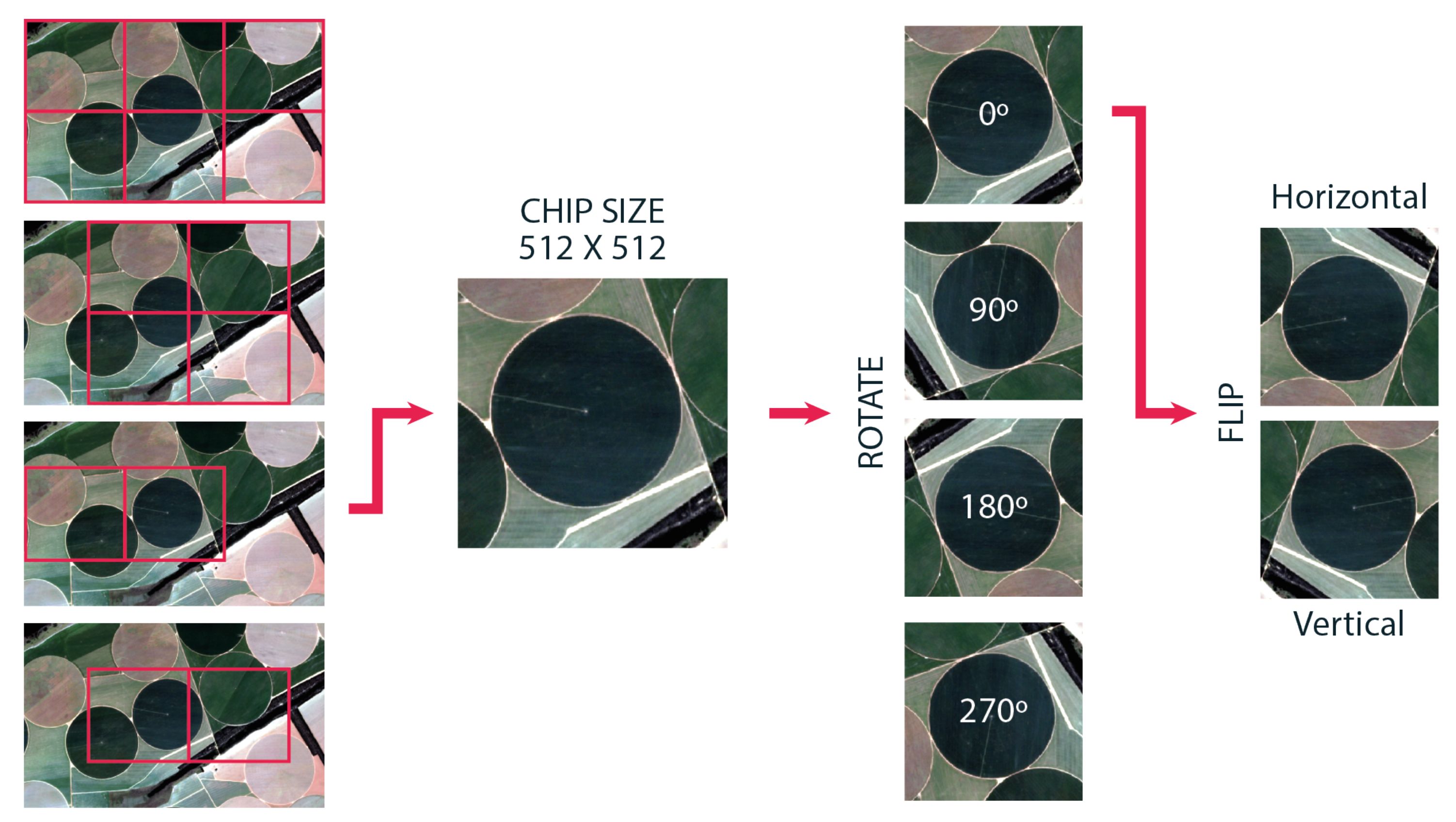
To extract the patches used to train the network, the first step is to run a sliding window of size 512 × 512 over each training image, using a step size of 256 in both dimensions. Patches that contain at least one pixel inside a center pivot irrigation system are used in training; the rest are discarded. The use of a step size that is half the size of the sliding window in both dimensions is a form of data augmentation that increases the amount of available data by nearly four times. Next, we normalize each patch using Z-score normalization [29]. The Z-score normalized value of each pixel in each band is defined by Equation (1).
Z i = x i μ σ ,
where x i is the value of the pixel in the band, μ is the average value for all pixels of that band in the patch, and σ is the standard deviation of the band in that patch. The result of Z-score normalization is that the data will be rescaled so that it will have the properties of a standard normal distribution, with an average of 0 and a standard deviation of 1. In image processing, data standardization is important not only when comparing measurements with different units, but also to allow for the classification of images with different value scales, and even those captured by different sensors after the training process.
After the patches are normalized, we apply data augmentation by rotation. Each patch is rotated by 90, 180, and 270 degrees. This increases the amount of available data by four times. Finally, we perform additional data augmentation by flipping the samples horizontally and vertically. When combined, these data augmentation techniques allow us to increase the size of our training dataset by approximately 48 times. A diagram of the data augmentation process is shown in Figure 4. After data augmentation, we got 4900 training samples, 727 validation samples, and 1059 test samples.

2.5. Training

We train our model to minimize the cross entropy between the pixel-wise softmax of the network’s output and the ground truth, using the NAdam [30] optimization algorithm with a learning rate of 0.00005, β 1 = 0.9, β 2 = 0.999, and ϵ = 1 × 10 8 . To reduce overfitting, we apply l 2 regularization with a scale of 0.01 to every kernel. We train the model with a batch size of 5 until the test and training errors stabilize. Training was performed on Google Cloud Platform using a machine with 4 cores, 50 GB of random access memory (RAM), and an NVIDIA Tesla K80 graphics processing unit (GPU). We validated the model at the end of every epoch, keeping a copy of the checkpoint with the lowest validation error.

2.6. Evaluation Metrics

We evaluated the performance of our model using four metrics: a c c u r a c y s c o r e , p r e c i s i o n , r e c a l l [31], and f 1 - s c o r e [32]. The accuracy score is the ratio of the correctly classified elements over all available elements. It is defined as
a c c u r a c y s c o r e = T P + T N T P + T N + F P + F N ,
where T P is the number of true positives, T N is the number of true negatives, F P is the number of false positives, and F N is the number of false negatives. This metric has a certain sensitivity to class imbalance, which occurs when small or sparse targets are identified. A more reliable metric in these situations is p r e c i s i o n (producer accuracy), which is the ratio of elements identified as members of a class to those which really belong to that class. The p r e c i s i o n is calculated as
p r e c i s i o n = T P T P + F P .
The r e c a l l (user accuracy) is the ratio of elements correctly identified as members of a class to all elements that belong to that class:
r e c a l l = T P T P + F N .
The f 1 - s c o r e is a metric that considers both the precision and the recall:
f 1 - s c o r e = 2 × p r e c i s i o n × r e c a l l p r e c i s i o n + r e c a l l .
We evaluated our results by performing a pixel-wise computation of all metrics; i.e., every pixel of every chip in the test set was classified as T P , T N , F P , or F N .

3. Results

The evolution of the training and validation errors of our model during the training process is shown in Figure 5. The training process took approximately 22 h to complete. The model’s loss showed great instability due to the size of our batch, which, due to computational limitations, was set to five. The use of a larger batch size would likely result in a more stable loss.
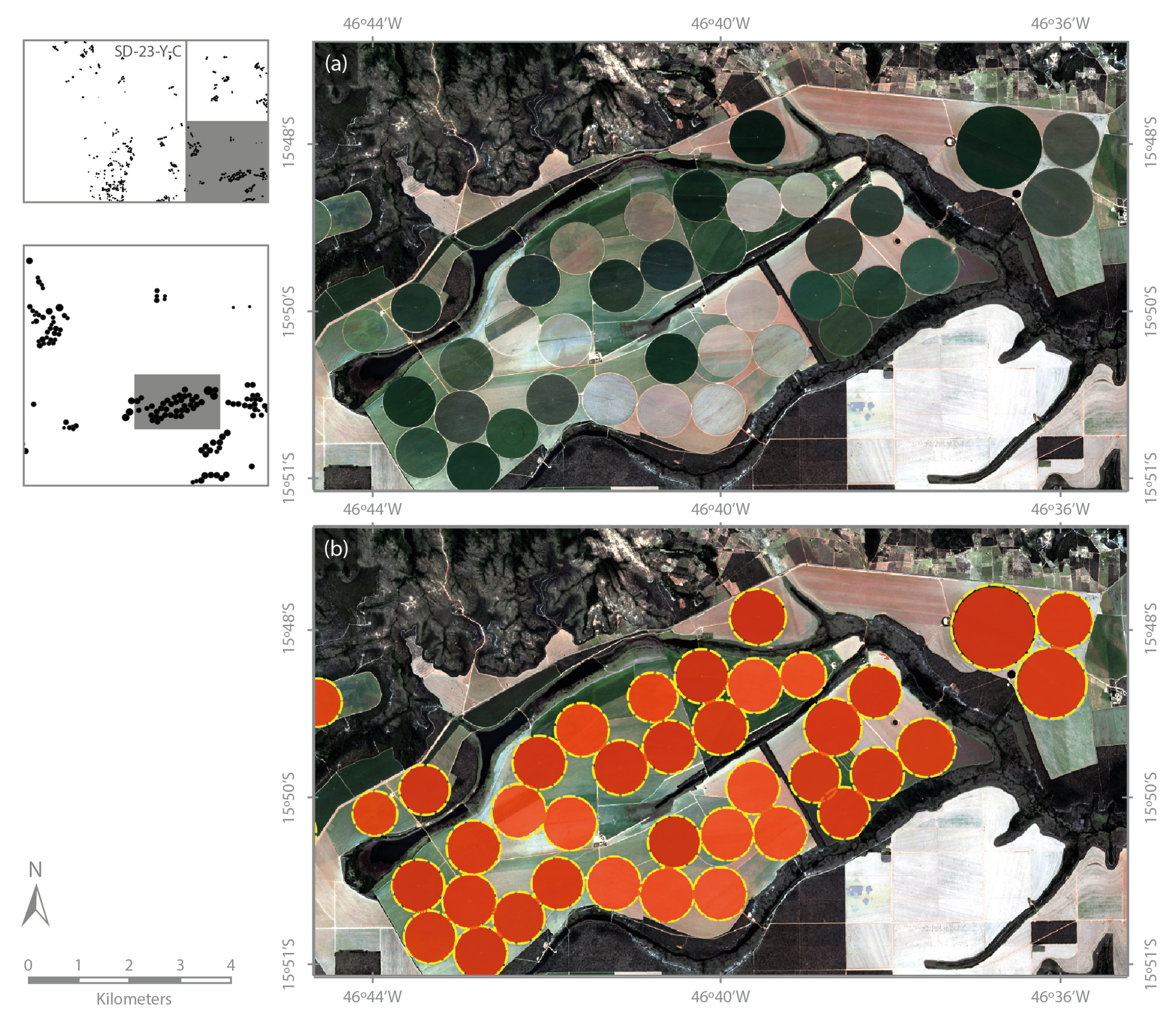
To evaluate the performance of our model, we used the set of U-Net weights that presented the lowest validation error during the entire training process. Our model was evaluated in a test set composed of 1059 labeled samples with 512 × 512 pixels that were not part of the training and validation sets. Table 1 presents the scores of our best modified U-Net model in all evaluation metrics. Qualitative results are shown in Figure 6 and Figure 7.
To test the generalization performance of our model, we applied it to a Landsat 8 OLI image acquired on 9 September 2019, for Path/Row 220/069 localized in the state of Bahia, Brazil. Unlike the training images, which are in TOA reflectance and have a spatial resolution of 3.7 m, this image is in digital number (DN) (a different scale) and has a spatial resolution of 30 m. A comparison between the two sensors is shown in Table 2. As we do not have reference data for this region, we could only perform a qualitative evaluation. Some results are shown in Figure 8.

4. Discussion

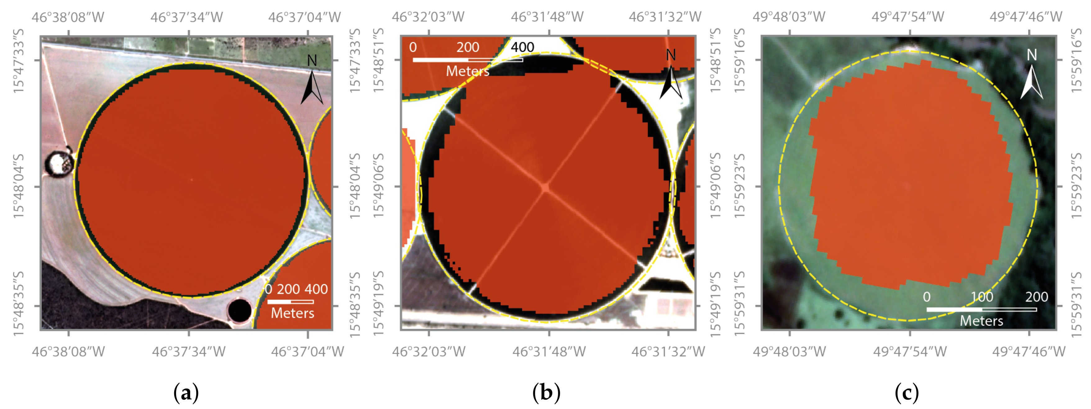
The results show a precision score above 99%, which indicates a low incidence of inclusion errors for Class 1, which corresponds to center pivot irrigation systems. Class 1 recall presented a score of 88%, the lowest among all metrics. This was mostly caused by the model leaving pixels at the edge of the pivots out of the segmentation mask, as shown in Figure 9. The scores above 99% in all metrics for Class 0 are mostly a result of the very large number of correctly labeled background pixels, which is also the main cause of the 99% accuracy score.
In grid SD-23-Y-C, our reference data, annotated by a specialist through visual inspection for the period of August 2017 to November 2018, contains 519 center pivot irrigation systems with a total area of 40,148 ha. In this area, our automatic detection method mapped 495 center pivots, including a false positive (a pivot that did not exist in the reference data), with a total area of 35,157 ha, an overall decrease of 12.43% in comparison to the reference map. In grid SD-22-Z-C, our reference data shows 114 center pivots with a total area of 7339 ha, 112 pivots of which were detected by our deep learning method. Our method also mapped a false positive, bringing the total to 113 center pivots with a total area of 6531 ha, 11.01% less than the reference data. The differences in the number of detected center pivots and total irrigated area between our results and the reference data can be attributed to imperfections in the segmentation mask, as shown in Figure 9, and omission and inclusion errors, exemplified in Figure 10.
One of the main advantages of convolutional neural networks in remote sensing applications is that, rather than considering just the images’ spectral values, these methods base their decisions on several factors, including the mapping target’s spatial context, texture, and shape, as well as more complex features that may not be obvious to human observers. Even though center pivot irrigation has a regular circular shape, it possesses high spectral and textural variability, making the automation of its detection and mapping a complex task. Figure 6 and Figure 7 present an example of how our modified U-Net algorithm is able to detect and map central pivot irrigation systems of different sizes and land cover, including areas of bare ground, earlier stages, and well-developed crops. Our model was able to successfully segment center pivot irrigation systems of different sizes, with radii between 190 and 950 m, which is a problem for the fixed size sliding window approach proposed by Zhang et al. [12]. It was also able to segment pivots that were only partially included in the test area. Our method, however, had some difficulty in segmenting irregularly shaped pivots.
The most common errors presented by our model are the cases shown in Figure 9a,b, where the network successfully identified the center pivot irrigation system, but failed to accurately segment its borders. Other common errors are shown in Figure 10. Figure 10a shows an irregularly shaped pivot that our network was unable to detect. We believe this kind of error was caused by the low occurrence of incomplete pivots in the training dataset and could be reduced by fine tuning the network to such cases. Another error of omission is shown in Figure 10c, where the network was unable to detect a center pivot with faint borders and irregular texture. Figure 10c,d present some inclusion errors caused by the model mistakenly identifying curved roads as edges of the center pivot irrigation system. These errors could probably be reduced by training the network with more examples of such cases.
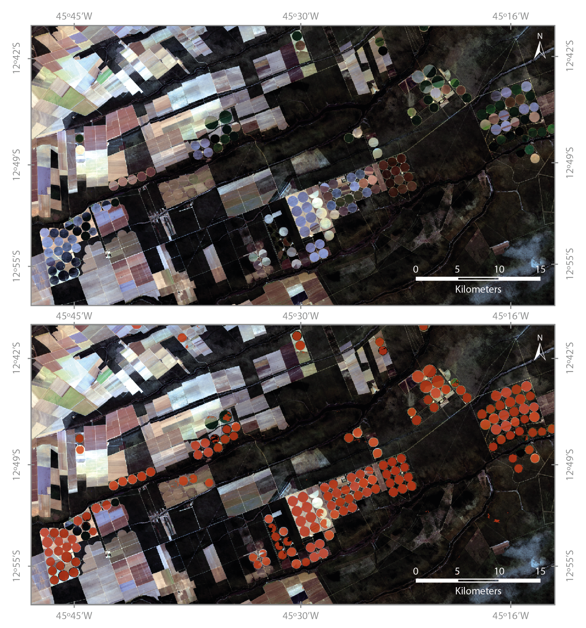
Figure 8 shows the results of the application of our model to a Landsat 8 OLI image. This image is in other location, with another sensor, spectral range, value scale, and spatial resolution, when compared to the data used to train the network. Despite this, our method was able to correctly segment most of the center pivot irrigation systems present in the image. This leads us to believe that our model was able to learn features that could be used to map center pivot irrigation systems in different regions. However, differences in land cover and crop characteristics, among other things, could lead to a significant reduction in segmentation performance in areas far from those used in the extraction of training samples. This could be fixed by retraining the network with samples extracted from regions with characteristics similar to those of the areas we wish to segment. We also believe that our methodology could be adapted to data captured with different sensors with minimal modifications to the network’s architecture.

5. Conclusions

We proposed a novel deep learning approach for the automatic detection and mapping of center pivot irrigation systems using satellite images using a modified U-Net image segmentation algorithm. The proposed method was able to locate, map, and quantify the center pivot irrigation systems within the study area, while also detecting pivots of different sizes with variable land cover and spatial texture. Our approach was capable of providing an estimation of the area equipped with center pivot irrigation systems in a large landscape. It also showed a good generalization performance, being able to work on inputs with different characteristics than those used to train the network. Our deep learning architecture took approximately 22 h to train and about 10 min to perform the segmentation of each grid of our study area. This is much faster, and consequently, cheaper than the manual segmentation by specialists. Our approach also proved to be capable of mapping central pivots of different sizes and in different stages of crop growth, which are problems for other automatic mapping methods reported in the literature. The method presented here can be used to map large areas in a relatively short time and at a relatively low cost, and provides a tool for monitoring the growth of the irrigated areas and the amount of installed center pivot irrigation equipment. This approach can be useful in the monitoring of irrigated agriculture systems and in the estimation of freshwater demand.

Author Contributions

Conceptualization, M.S. (Marciano Saraiva) and M.S. (Moisés Salgado); Methodology, M.S. (Marciano Saraiva), É.P. and M.S. (Moisés Salgado); Software, M.S. (Marciano Saraiva) and É.P.; Validation, M.S. (Marciano Saraiva) and É.P.; Formal analysis, M.S. (Marciano Saraiva), É.P. and M.S. (Moisés Salgado); Investigation, M.S. (Marciano Saraiva), É.P. and M.S. (Moisés Salgado); Resources, C.S.J.; Data curation, M.S. (Marciano Saraiva) and É.P.; Writing—Original draft preparation, M.S. (Marciano Saraiva) and É.P.; Writing—Review and editing, M.S. (Moisés Salgado) and C.S.J.; Visualization, M.S. (Marciano Saraiva), É.P., M.S. (Moisés Salgado) and C.S.J.; Supervision, C.S.J.; Project administration, M.S. (Moisés Salgado); Funding acquisition, C.S.J. All authors have read and agreed to the published version of the manuscript.

Funding

This work, part of the MapBiomas and NextGenMap initiatives, was supported by the Gordon and Betty Moore Foundation.

Acknowledgments

We would like to thank the Gordon and Betty Moore Foundation for funding, Planet for providing the access to daily PlanetScope imagery, and Google for the processing infrastructure made available to the project.

Conflicts of Interest

The authors declare that there is no conflict of interest.

References

  1. Rosegrant, M.W.; Cai, X. Global Water Demand and Supply Projections. Water Int. 2002, 27, 170–182. [Google Scholar] [CrossRef]
  2. Frenken, K.; Gillet, V. Irrigation Water Requirement and Water Withdrawal by Country; FAO: Rome, Italy, 2012. [Google Scholar]
  3. Singh, A. Decision support for on-farm water management and long-term agricultural sustainability in a semi-arid region of India. J. Hydrol. 2010, 391, 63–76. [Google Scholar] [CrossRef]
  4. Yu, Y.; Disse, M.; Yu, R.; Yu, G.; Sun, L.; Huttner, P.; Rumbaur, C. Large-Scale Hydrological Modeling and Decision-Making for Agricultural Water Consumption and Allocation in the Main Stem Tarim River, China. Water 2015, 7, 2821–2839. [Google Scholar] [CrossRef] [Green Version]
  5. Chen, Y.; Ye, Z.; Shen, Y. Desiccationof the Tarim River, Xinjiang, China, and mitigation strategy. Quat. Int. 2011, 244, 264–271. [Google Scholar] [CrossRef]
  6. Liu, Y.; Song, W.; Deng, X. Spatiotemporal Patterns of Crop Irrigation Water Requirements in the Heihe River Basin, China. Water 2017, 9, 616. [Google Scholar] [CrossRef] [Green Version]
  7. Instituto Brasileiro de Geografia e Estatística. Censo Agropecuário 2017: Resultados Preliminares; Instituto Brasileiro de Geografia e Estatística: Rio de Janeiro, Brazil, 2017. [Google Scholar]
  8. Agência Nacional de Águas. Levantamento da Agricultura Irrigada por Pivôs Centrais no Brasil, 2nd ed.; Agencia Nacional de Aguas (ANA): Brasilia, Brazil, 2019. [Google Scholar]
  9. Carlson, M.P. The Nebraska Center-Pivot Inventory: An example of operational satellite remote sensing on a long-term basis. Photogramm. Eng. Remote Sens. 1989, 55, 587–590. [Google Scholar]
  10. Duda, R.O.; Hart, P.E. Use of the Hough Transformation to Detect Lines and Curves in Pictures; Technical Report; SRI International Menlo Park CA Artificial Intelligence Center: Menlo Park, CA, USA, 1971. [Google Scholar]
  11. Yan, L.; Roy, D. Automated crop field extraction from multi-temporal Web Enabled Landsat Data. Remote Sens. Environ. 2014, 144, 42–64. [Google Scholar] [CrossRef] [Green Version]
  12. Zhang, C.; Yue, P.; Di, L.; Wu, Z. Automatic Identification of Center Pivot Irrigation Systems from Landsat Images Using Convolutional Neural Networks. Agriculture 2018, 8, 147. [Google Scholar] [CrossRef] [Green Version]
  13. LeCun, Y.; Bottou, L.; Bengio, Y.; Haffner, P. Gradient-based learning applied to document recognition. Proc. IEEE 1998, 86, 2278–2324. [Google Scholar] [CrossRef] [Green Version]
  14. Krizhevsky, A.; Sutskever, I.; Hinton, G.E. Imagenet classification with deep convolutional neural networks. In Advances in Neural Information Processing Systems; MIT Press: Cambridge, MA, USA, 2012; pp. 1097–1105. [Google Scholar]
  15. Simonyan, K.; Zisserman, A. Very deep convolutional networks for large-scale image recognition. arXiv Prepr. 2014, arXiv:1409.1556. [Google Scholar]
  16. Planet Labs. Planet Imagery Product Specification: PlanetScope & RapidEye. 2016. Available online: https://assets.planet.com/docs/combined-imagery-product-spec-april-2019.pdf (accessed on 1 November 2019).
  17. Neelakantan, A.; Vilnis, L.; Le, Q.; Sutskever, I.; Kaiser, L.; Kurach, K.; Martens, J. Adding Gradient Noise Improves Learning for Very Deep Networks. arXiv 2015, arXiv:1511.06807v1. [Google Scholar]
  18. Koziarski, M.; Cyganek, B. Image recognition with deep neural networks in presence of noise–dealing with and taking advantage of distortions. Integr. Comput. Aided Eng. 2017, 24, 337–349. [Google Scholar] [CrossRef]
  19. Gorelick, N.; Hancher, M.; Dixon, M.; Ilyushchenko, S.; Thau, D.; Moore, R. Google Earth Engine: Planetary-scale geospatial analysis for everyone. Remote Sens. Environ. 2017, 202, 18–27. [Google Scholar] [CrossRef]
  20. Hastie, T.; Tibshirani, R.; Friedman, J.; Franklin, J. The elements of statistical learning: Data mining, inference and prediction. Math. Intell. 2005, 27, 222–223. [Google Scholar]
  21. Ronneberger, O.; Fischer, P.; Brox, T. U-net: Convolutional networks for biomedical image segmentation. In International Conference on Medical Image Computing and Computer-Assisted Intervention; Springer: Berlin, Germany, 2015; pp. 234–241. [Google Scholar]
  22. Arganda-Carreras, I.; Turaga, S.C.; Berger, D.R.; Cireşan, D.; Giusti, A.; Gambardella, L.M.; Schmidhuber, J.; Laptev, D.; Dwivedi, S.; Buhmann, J.M.; et al. Crowdsourcing the creation of image segmentation algorithms for connectomics. Front. Neuroanat. 2015, 9, 142. [Google Scholar] [CrossRef] [PubMed]
  23. Maška, M.; Ulman, V.; Svoboda, D.; Matula, P.; Matula, P.; Ederra, C.; Urbiola, A.; España, T.; Venkatesan, S.; Balak, D.M.; et al. A benchmark for comparison of cell tracking algorithms. Bioinformatics 2014, 30, 1609–1617. [Google Scholar] [CrossRef] [PubMed]
  24. Iglovikov, V.; Mushinskiy, S.; Osin, V. Satellite Imagery Feature Detection using Deep Convolutional Neural Network: A Kaggle Competition. arXiv 2017, arXiv:1706.06169. [Google Scholar]
  25. Feng, W.; Sui, H.; Huang, W.; Xu, C.; An, K. Water Body Extraction From Very High-Resolution Remote Sensing Imagery Using Deep U-Net and a Superpixel-Based Conditional Random Field Model. IEEE Geosci. Remote Sens. Lett. 2018, PP, 1–5. [Google Scholar] [CrossRef]
  26. Pan, X.; Yang, F.; Gao, L.; Chen, Z.; Zhang, B.; Fan, H.; Ren, J. Building Extraction from High-Resolution Aerial Imagery Using a Generative Adversarial Network with Spatial and Channel Attention Mechanisms. Remote Sens. 2019, 11, 917. [Google Scholar] [CrossRef] [Green Version]
  27. Ioffe, S.; Szegedy, C. Batch Normalization: Accelerating Deep Network Training by Reducing Internal Covariate Shift. In Proceedings of the International Conference on Machine Learning, Lille, France, 6–11 July 2015; pp. 448–456. [Google Scholar]
  28. Abadi, M.; Agarwal, A.; Barham, P.; Brevdo, E.; Chen, Z.; Citro, C.; Corrado, G.S.; Davis, A.; Dean, J.; Devin, M.; et al. TensorFlow: Large-Scale Machine Learning on Heterogeneous Systems. 2015. Available online: www.tensorflow.org (accessed on 1 November 2019).
  29. Kreyszig, E. Advanced Engineering Mathematics, 4th ed.; John Wiley and Sons Ltd.: Hoboken, NJ, USA, 1979; p. 880. [Google Scholar]
  30. Dozat, T. Incorporating nesterov momentum into adam. In Proceedings of the ICLR, San Juan, Puerto Rico, 2–4 May 2016. [Google Scholar]
  31. Fernandez-Moral, E.; Martins, R.; Wolf, D.; Rives, P. A new metric for evaluating semantic segmentation: Leveraging global and contour accuracy. In Proceedings of the IEEE Intelligent Vehicles Symposium (IV), Suzhou, China, 26–30 June 2018; pp. 1051–1056. [Google Scholar]
  32. Rijsbergen, C.J.V. Information Retrieval, 2nd ed.; Butterworth-Heinemann: Newton, MA, USA, 1979. [Google Scholar]
  33. Planet Labs. Planet Imagery Product Specifications. 2019. Available online: https://www.planet.com/products/satellite-imagery/files/1610.06_Spec%20Sheet_Combined_Imagery_Product_Letter_ENGv1.pdf (accessed on 1 November 2019).
  34. U.S. Geological Survey. Landsat 8 (L8) Data Users Handbook; U.S. Geological Survey: Reston, VA, USA, 2019. [Google Scholar]
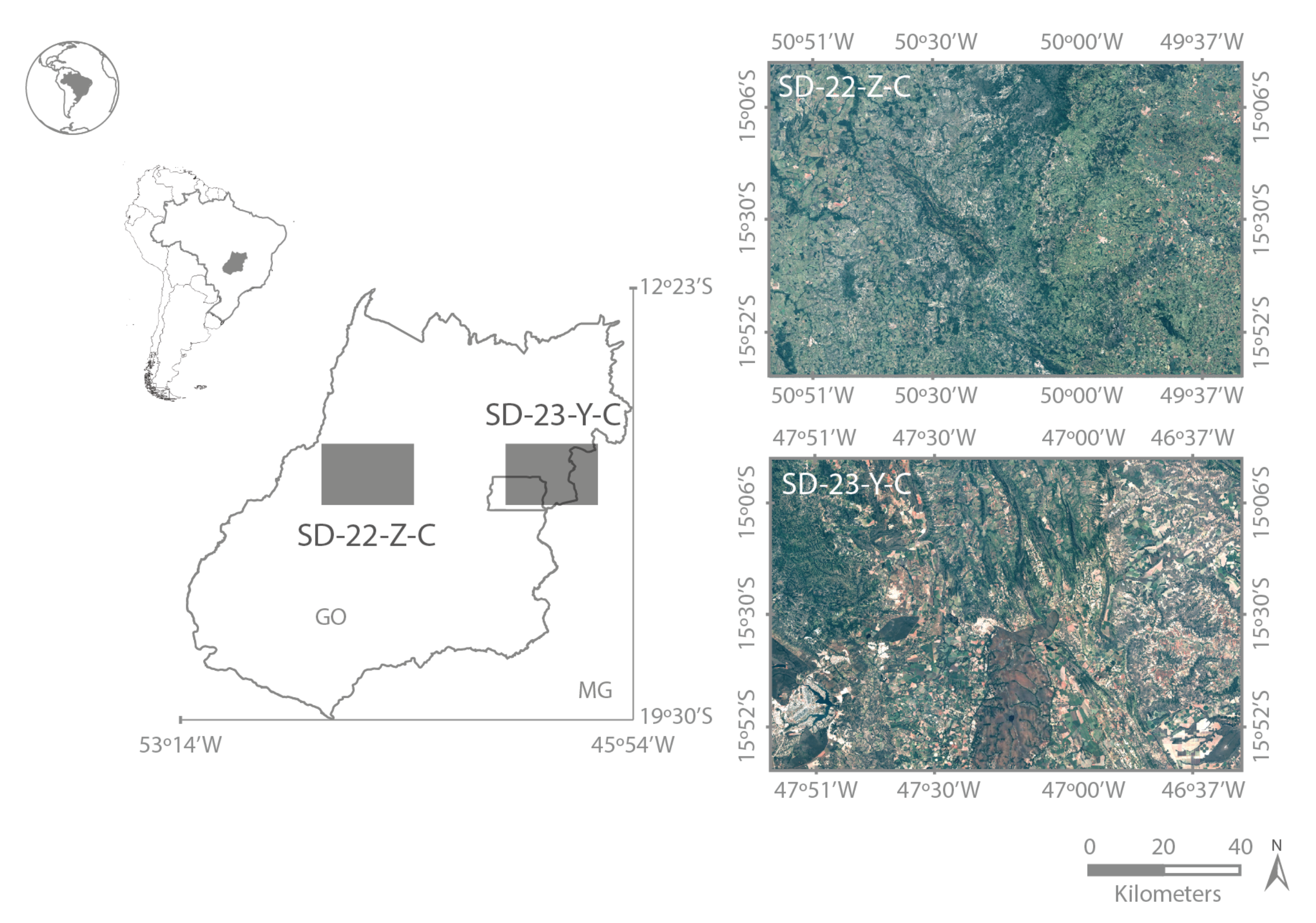
Figure 1. Spatial location of grids SD-23-Y-C and SD-22-Z-C.
Remotesensing 12 00558 g001
Figure 2. Samples collected in Regions A and B were used during the training process to train and to validate the model, respectively. The samples collected in Region C were used to evaluate the model during the accuracy analysis. Labeled center pivot irrigation systems are shown in black.
Remotesensing 12 00558 g002
Figure 3. Original and modified U-net architectures (example for 32 × 32 pixels in the lowest resolution). Each blue box corresponds to a multi-channel feature map. The number of channels is denoted on top of the box. The x-y-size is provided at the lower left edge of the box. White boxes represent copied feature maps. The arrows denote the different operations. Based on Figure 1 from [21]. (a) Original U-Net architecture [21]; (b) Modified U-Net architecture
Remotesensing 12 00558 g003
Figure 4. Data augmentation process. For each training image, we extracted 512 × 512 patches with a step size of 256 pixels. We rotated each patch by 90, 180, and 270 degrees, increasing the amount of available data by four times. Finally, we flipped all patches, including the ones produced by rotation, horizontally and vertically. In total, our data augmentation strategy increased the amount of training samples by 48 times.
Remotesensing 12 00558 g004
Figure 5. The network’s training losses. Orange lines represent the loss on the training set; blue lines represent the loss on the validation set.
Remotesensing 12 00558 g005
Figure 6. Results for an area of grid SD-23-Y-C-5 in the Brazilian Continuous Cartographic Base, located in the municipality of Unaí, in the estate of Minas Gerais. (a) PlanetScope median mosaic, in true color composition, built using images from the period of August 2017 to November 2018; (b) comparison between the reference (yellow dotted lines) and our results (red).
Remotesensing 12 00558 g006
Figure 7. Results for an area of grid SD-22-Z-C-5 in the Brazilian Continuous Cartographic Base, located in the municipalities of Goiás and Itaberaí, in the state of Goiás. (a) PlanetScope median mosaic, in true color composition, built using images from the period from August 2017 to November 2018; (b) comparison between the reference (yellow dotted lines) and our results (red).
Remotesensing 12 00558 g007
Figure 8. Results of the application of our model, trained in PlanetScope images, to a Landsat 8 OLI image localized in the state of Bahia, Brazil. The input image is shown at the top, and the results of the automatic mapping, in red, are at the bottom.
Remotesensing 12 00558 g008
Figure 9. Examples of center pivot irrigation system segmentation using our approach. The yellow dotted lines show the position of center pivot irrigation systems in the reference data, and the results of the automatic mapping using our approach are shown in red. (a) Accurate segmentation mask; (b) Some pixels at the edge are left out; (c) Many pixels at the edge are incorrectly classified.
Remotesensing 12 00558 g009
Figure 10. Examples of segmentation errors using our approach. The areas classified as center pivots are shown in red. (a) Omission error likely caused by irregular shape; (b) Omission error caused by faint borders; (c,d) Inclusion error caused by curved roads.
Remotesensing 12 00558 g010
Table 1. Validation of results of our model using the set of weights with the lowest test error. Class 0 represents the background, and Class 1 corresponds to center pivot irrigation systems.
Class Precision (Producer Accuracy) Recall (User Accuracy) F 1 - Score Accuracy Score
10.990.880.930.99
00.990.990.99
Table 2. Comparison between PlaneScope [33] and Landsat 8 [34] sensors.
PlanetScopeLandsat 8
Sensor namePS2.SDOperational Land Imager—OLI
Spatial resolution3.7 m30 m
Spectral bandsBlue 0.45–0.51 μ m
Green 0.50–0.59 μ m
Red 0.59–0.67 μ m
NIR 0.78–0.86 μ m
Blue 0.45–0.51 μ m
Green 0.53–0.59 μ m
Red 0.64–0.67 μ m
NIR 0.85–0.88 μ m
Pixel valueTOADigital Number
Radiometric resolution16 bit12 bit