Article

Spatial Habitat Shifts of Oceanic Cephalopod (Ommastrephes bartramii) in Oscillating Climate

1
Arctic Research Center, Hokkaido University, N21 W11 Kita-Ku, Sapporo 001-0021, Japan
2
Data Research Center for Marine-Earth Sciences, Japan Agency for Marine Earth-Science and Technology, JAMSTEC, 3173-25 Showamachi, Kanazawa-ward Yokohama City, Kanagawa 236-0001, Japan
3
Fisheries Research Institute, Aomori Prefectural Industrial Technology Research Center, Hiranai, Aomori 039-3381, Japan
*
Author to whom correspondence should be addressed.
Remote Sens. 2020, 12(3), 521; https://doi.org/10.3390/rs12030521
Submission received: 12 December 2019 / Revised: 17 January 2020 / Accepted: 1 February 2020 / Published: 5 February 2020
(This article belongs to the Special Issue Remote Sensing for Fisheries and Aquaculture)

Abstract

:
Short- and long-term climate oscillations impact seascapes, and hence, marine ecosystem structure and dynamics. Here, we explored the spatio-temporal patterns of potential squid habitat in the western and central North Pacific across inter-decadal climate transitions, coincident with periods of persistent warming and cooling. Potential habitat distributions of Ommastrephes bartramii were derived from the outputs of multi-ensemble species distribution models, developed using the most influential environmental factors to squid distribution and occurrence data. Our analyses captured the underlying temporal trends in potential squid habitat in response to environmental changes transpiring at each climatic transition, regulated by phase shifts in Pacific decadal oscillation (PDO) from 1999–2013. The spatial differences in environmental conditions were apparent across transitions and presumably modulate the local changes in suitable squid habitat over time. Specifically, during a cold to warm PDO shift, decreases in the summer potential habitat (mean rate ± standard deviation: −0.04 ± 0.02 habitat suitability index (HSI)/yr) were observed along the southern edge of the subarctic frontal zone (162°E–172°W). Coincidentally, this area also exhibits a warming trend (mean temporal trend: 0.06 ± 0.21 °C/yr), accompanied with the prevalence of cold-core mesoscale eddies, west of the dateline (mean temporal trend in sea surface height: −0.19 ± 1.05 cm/yr). These conditions potentially generate less favorable foraging habitat for squid. However, a warm-to-cold PDO transition underpins a northward shift of suitable habitat and an eastward shift of regions exhibiting the highest rate of potential squid habitat loss (170–160°W; mean temporal trend: −0.05 ± 0.03 HSI/yr). Nonetheless, the emergence of the areas with increasingly suitable habitat regardless of climate transitions suggests the ecological importance of these regions as potential squid habitat hotspots and climatic refugia.

Graphical Abstract

1. Introduction

Neon flying squid (Ommastrephes bartramii) is a large epipelagic cephalopod widely distributed across the subtropical and temperate oceans [1]. It is among the internationally (e.g., Japan, China, South Korea and Taiwan) exploited fishery resources of high commercial value in the North Pacific [2,3]. It has an averaged capture production amounting to 19,245 tonnes from 2001–2010 and is one of the major squid species comprising the world capture production of cephalopods for this decade [4]. Multinational industrial fishery started when the catches of the Japanese flying squid (Todarodes pacificus) experienced a dramatic downturn in the 1970s and commercial harvests of the neon flying squid in the North Pacific waters proceeded since then [3].
O. bartramii population in the North Pacific Ocean encompasses two seasonal cohorts: winter-spring and autumn spawning groups [5]. Their spatial and temporal distributions are linked with the basin-wide oceanic circulation and their life history stages are highly responsive to the variability in ambient oceanographic regimes and concomitant changes in epipelagic environment [6,7,8]. Furthermore, both squid cohorts undergo extensive seasonal and meridional migrations between their spawning (subtropical region; 20–30°N) and foraging sites (Kuroshio–Oyashio transition and subarctic frontal zones; 30–50°N), within their brief 1-year life-span (Figure 1A) [5,9,10]. Concurrent with its summer feeding migration, industrial Japanese fishing activities primarily occur in the offshore waters of the western and central North Pacific (Figure 1B). In an ecological context, O. bartramii adopts significant roles in the epipelagic ecosystems owing to its mid-trophic position in oceanic food webs. Previous work on the feeding habits and diet of neon flying squid revealed that it is an opportunistic/generalist feeder that preys on crustaceans, small mesopelagic fishes and other cephalopods. It is also a major prey item for larger predators and is, hence, thought to create vital mid-level trophic links between animals of tertiary trophic level and apex predators [11,12,13].
A growing number of research points to the significance of looking into regional and short- to mid-term patterns in species’ habitat distributions, as interactions of environmental gradients vary across multiple spatio-temporal scales [14,15,16]. In particular, habitat distribution patterns in marine ecosystems are largely dictated by the species’ sensitivity to diverse environmental and climatic cues. As cephalopods are generally short-lived taxa, they are known to swiftly respond to drastic climate and environmental perturbations, thus, making them effective biological sentinel of climatic changes [17,18]. In light of the rapidly changing climate, sentinel species can provide valuable information on ecosystem function, distinguish ocean and human health-related risks and forecast future changes [19,20,21]. Taking these characteristics into account and building upon the results of our foregoing work [6,22,23], we hereby extended our present analyses of squid–environment interactions to implement a simple yet ecologically pertinent approach to quantify the changes in potential squid habitat in the North Pacific under the recent thermal regimes, marked by distinct phase transitions of the Pacific decadal oscillation (PDO) between 1999 and 2013. Here, we used the outputs from the multi-model habitat ensemble to infer the potential squid habitat over a 15-year period and quantify the rates of habitat change across different PDO-governed thermal regimes. In doing so, we were able to evaluate the spatial changes of potential squid habitat distributions in response to the decadal shifts in the dominant year-round pattern of sea surface temperature (SST) variability in the North Pacific Ocean.
Furthermore, our analyses, albeit on a shorter time-scale relative to earlier studies on climate refugia [24,25], provided some insights on potential sites that could act as open-ocean refugia under changing environmental conditions in the western and central North Pacific Ocean. In the literature, climate refugia are increasingly recognized for their importance in ecology and conservation studies, as they facilitate the persistence of biodiversity under changing climates [24,25]. While this concept has been broadly investigated in terrestrial ecosystems, identification of these sites in aquatic and marine systems could assist conservation efforts and spatial planning in a changing ocean climate. In the global ocean, climate refugia are generally characterized by areas where some or all variables influenced by climate variability exhibit the least changes and often overlap with oceanographic features that preclude climate change exposure [26]. Examples of these oceanographic features are seamounts and persistent frontal structures that create retention areas and habitat hotspots for many marine species [27,28,29]. In the present study, potential local refugia, referred to sites where the inferred squid habitat exhibited increasing trends regardless of the PDO phase transitions.
Overall, this study seeks to examine the spatial patterns of temporal trends in potential squid habitat in the North Pacific over the 15-year period, punctuated by persistent warm and cold phases of PDO-associated oceanographic regimes. Specifically, we aim to (1) estimate the annual changes in habitat suitability for the neon flying squid from late spring to summer (May–July) in the western and central North Pacific, across contrasting PDO phase transitions, and (2) identify climatically-sensitive zones to shifting contemporary patterns of oceanographic conditions and suitable climatic squid habitat over time.

2. Materials and Methods

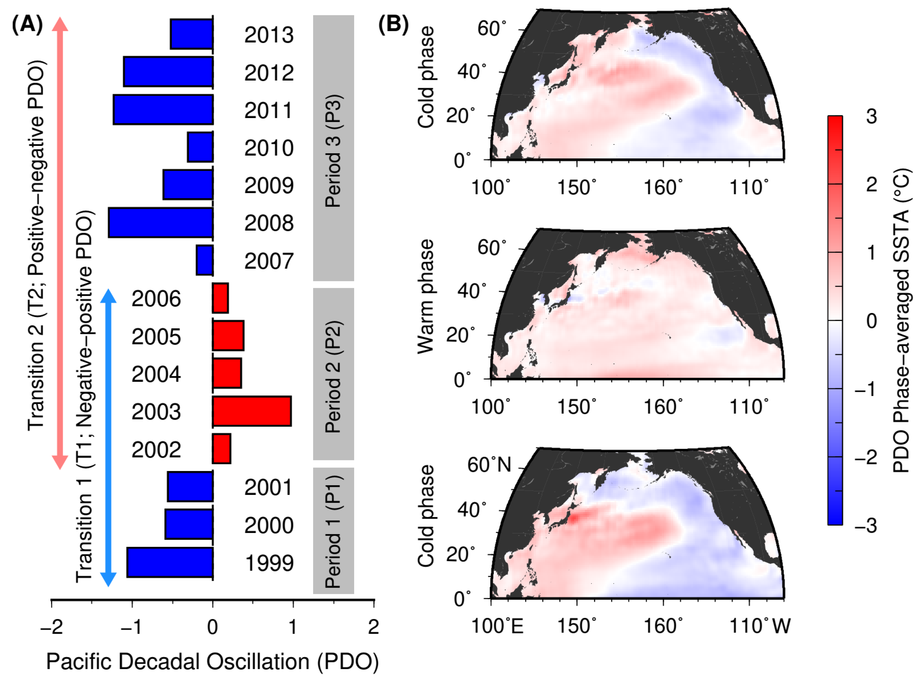
2.1. Pacific Decadal Oscillation (PDO)-Based Climatic Phase Shifts

During the duration of study, climate transitions were identified based on the patterns of Pacific decadal oscillation (PDO) from January to December, 1999–2013 (Figure 2A). The PDO was initially introduced by [30] as the leading empirical orthogonal function (EOF) of the North Pacific (20°–70°N) SST monthly averaged anomalies (SSTAs). The anomalies were computed as the departures from the climatological annual cycle after the removal of global mean SSTs. Since its introduction, PDO has been linked to the other components of the climate system [31] and to its profound impacts on marine ecosystems and fisheries [30,32,33].
Here, monthly PDO data were downloaded from the Joint Institute for the Study of Atmosphere and Ocean (JISAO) (http://research.jisao.washington.edu/pdo/PDO.latest.txt, date accessed: 20 June 2017). The monthly time-series data were annually-averaged and plotted to visually identify PDO patterns. The annual averages of PDO index were used for the analyses as the neon flying squid has a one-year life-span [5,11], and thus, this temporal resolution better captures the climate conditions experienced by the species throughout its lifetime. Similarly, monthly sea surface temperature (SST) anomaly data computed using a 30-year base period (1971–2000) were from the International Research Institute for Climate and Society (IRI) (iridl.ldeo.columbia.edu/SOURCES/.NOAA/.NCEP/.EMC/.CMB/.GLOBAL/.Reyn_SmithOIv2/.monthly/.ssta, date accessed: 20 June 2017). The data were used to examine the corresponding spatial SSTA patterns at each respective PDO phase. Due to the long-lived and year-long SST-based climate variability pattern associated with PDO signals [31,34], we were able to capture two PDO phase transitions within our study period (Figure 2A). Each of the periods within a given transition was represented by a basin-wide warming or cooling (Figure 2B). Here, transition 1 (T1) is defined by a shift from the cold (period 1, P1; 1999–2001) to warm (period 2, P2; 2002–2006) phase and transition 2 (T2) is characterized by a shift on opposite direction, from warm (P2) to cold PDO phase (period 3, P3; 2007–2013).

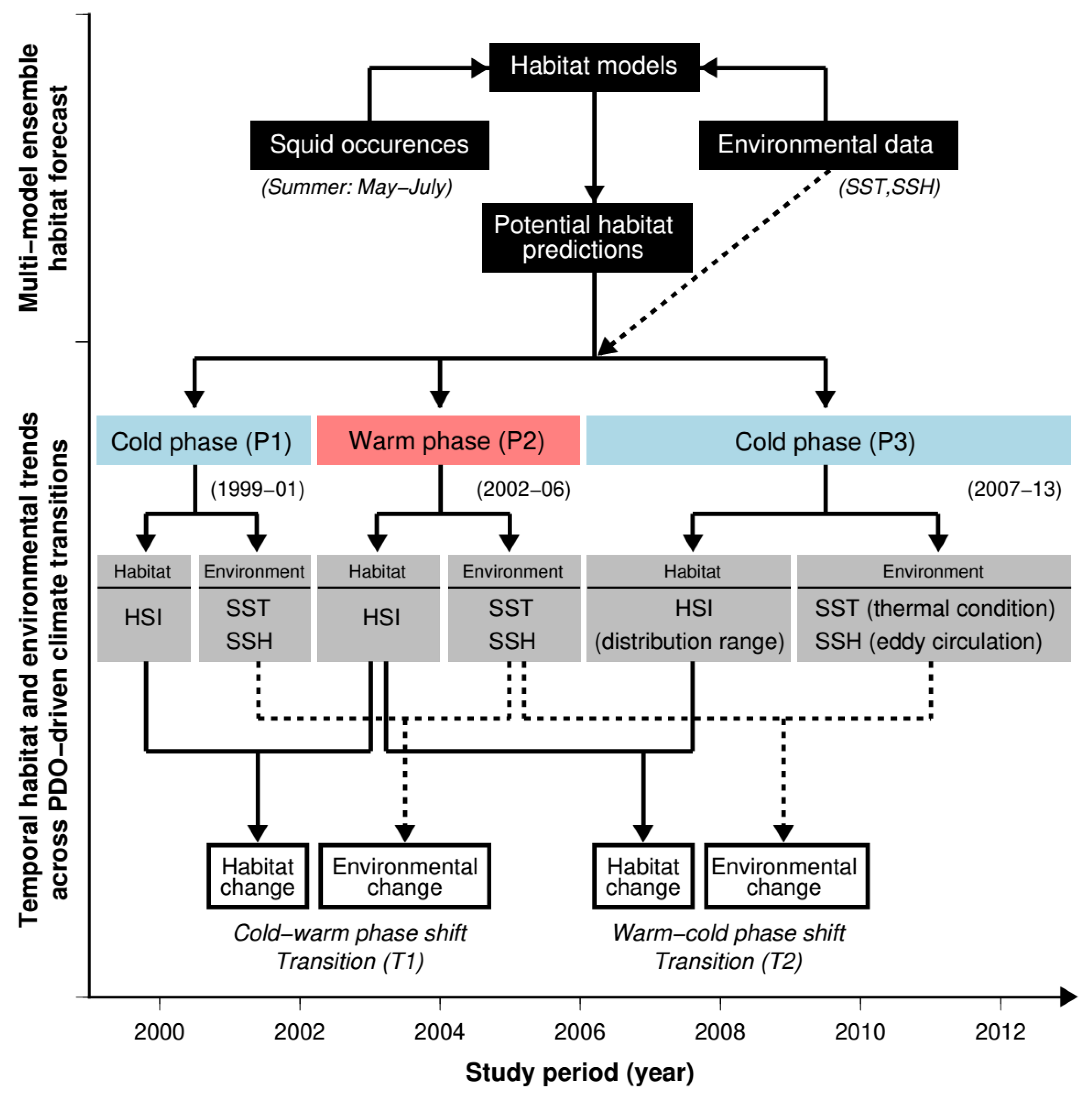
2.2. Analytical Framework

Our analyses were implemented following the framework proposed in Figure 3. Here, multi-model habitat forecasts were generated using the monthly-pooled (May–July) information of squid occurrences and set of most influential environmental factors (i.e. sea surface temperature, SST and sea surface height, SSH) to squid habitat distribution. These variables are related to the thermal and mesoscale environments, respectively, that significantly impact the summer feeding areas for squid and other pelagic species. Annual seasonal averages of multi-model habitat predictions (May–July, 1999–2013) were computed and temporal trends for each climatic transition between two consecutive periods of PDO-specific phase were then calculated. These calculations were also carried out for SST and SSH to examine the rates at which the thermal and mesoscale environments were changing across PDO phase transitions. Finally, comparison of spatial patterns between temporal trends for potential squid habitat and oceanographic conditions was undertaken to identify areas that are particularly sensitive to climatic changes.

2.3. Squid Occurrences and Environmental Data

The monthly-compiled squid jigging vessel positions (Longitude, Latitude) from daily fishing logs (point data) from May to July 1999–2013 (corresponding to Japanese commercial jigging months in summer, Figure 1B) were provided by the Aomori Prefectural Industrial Technology Research Center (APITRC). The environmental variables used for the habitat model construction comprised the monthly-averaged sea surface temperature (SST) computed from the daily optimally-interpolated Advanced Very High Resolution Radiometer- Optimally interpolated (AVHRR-OI) SST (ftp.podaac-ftp.jpl.nasa.gov/allData/ghrsst/data/L4/GLOB/NCDC/AVHRR_OI/; date accessed: 4 February 2016) and monthly-averaged sea surface height (SSH) calculated from daily-resolved altimeter measurements from the Archiving, Validation and Interpretation of Satellite Oceanographic data (AVISO) website (ftp.aviso.oceanobs.com; date accessed: 4 February 2016) between May and July 1999–2013. The selection of environmental variables used in the analyses were supported by the results of earlier studies, suggesting that these factors were most influential to squid habitat distributions [22,23,35]. All the environmental data were resampled to a common spatial resolution (0.25° × 0.25°) prior to habitat model construction and subsequent analyses. Finally, using a bicubic interpolation [36], the grid at each fishing point location was also interpolated (0.25° × 0.25°) to extract the corresponding environmental values at the given fishing position.

2.4. Multi-Model Ensemble of Potential Squid Habitat

Using a set of environmental factors and squid occurrences, a total of 10 single-algorithm models available within the BIOMOD2 r package [37] were trained and fitted to predict the species habitat distributions in the study area. BIOMOD2 invokes regression and machine-learning based presence-only models to compute for the habitat suitability index (HSI), where values close to or equal to 1 suggest areas of favorable species habitat. The parametrizations and settings used for the development of the single-algorithm models are summarized in Table 1.
Since the pixels with no squid jigging activity cannot be classified as true absences, a total of 500 pseudo-absences for each squid jigging observation compiled daily were randomly selected across all environmental layers. These data were then pooled together across each period and final pseudo-absences used for subsequent single-algorithm model runs were randomly subsampled from the pooled data using a 1:10 presence to pseudo-absence ratio [38]. The random sub-sampling of pseudo-absences was carried out to make model simulations computationally feasible yet within a moderate sampling prevalence [39]. The subsequent selection of the single-algorithm models used to generate a weighted mean multi-model ensemble was based on an arbitrary threshold for the true skill statistic (TSS). As there is no known consensus yet as to the most appropriate evaluation metric for ensemble forecasts [40], we used the TSS for model selection (TSS ≥ 0.80; Table 2). Unlike the other performance metrics (area under the curve (AUC) and Cohen’s Kappa, hereafter Kappa), TSS is independent of the model prevalence and thus, provides a more robust measure [41]. Here, the weights for ensemble model were proportional to the computed TSS of best-performing models [37]. Finally, the compiled occurrences at each given period were randomly divided into training (70%) and testing (30%) sets, for fitting and evaluating the models, respectively.

2.5. Computing for Temporal Trends at Each Climatic Transition

The temporal trend for potential squid habitat at each PDO phase transition between successive periods Figure 2), correspond to the slope of the cell-wise linear regressions between HSI and year, as response and independent variables, respectively. This calculation was also performed for environmental parameters (SST and SSH) against year at each given phase transition. Doing so enables us to quantify the magnitude and direction of habitat and environmental changes across space under different PDO phase transitions. All the analyses were performed in R version 3.6.0 [42] and all the mapping routines were carried out using general mapping tools (GMT) version 4.5.15 [36].
Moreover, to identify potential local refugia, we classified the temporal trends for HSI, SST and SSH in areas with the highest predicted squid habitat (165°E–160°W and 39–46°N) into equal quintiles, resulting into five categories of habitat and oceanographic changes at each transition (Table 3): large decrease, small decrease, largely unchanged, small increase, and large increase [26]. Subsequently, we mapped and examined the spatial overlap of small and large increases in HSI with, classified maps of SST and SSH at each PDO phase transition.

3. Results

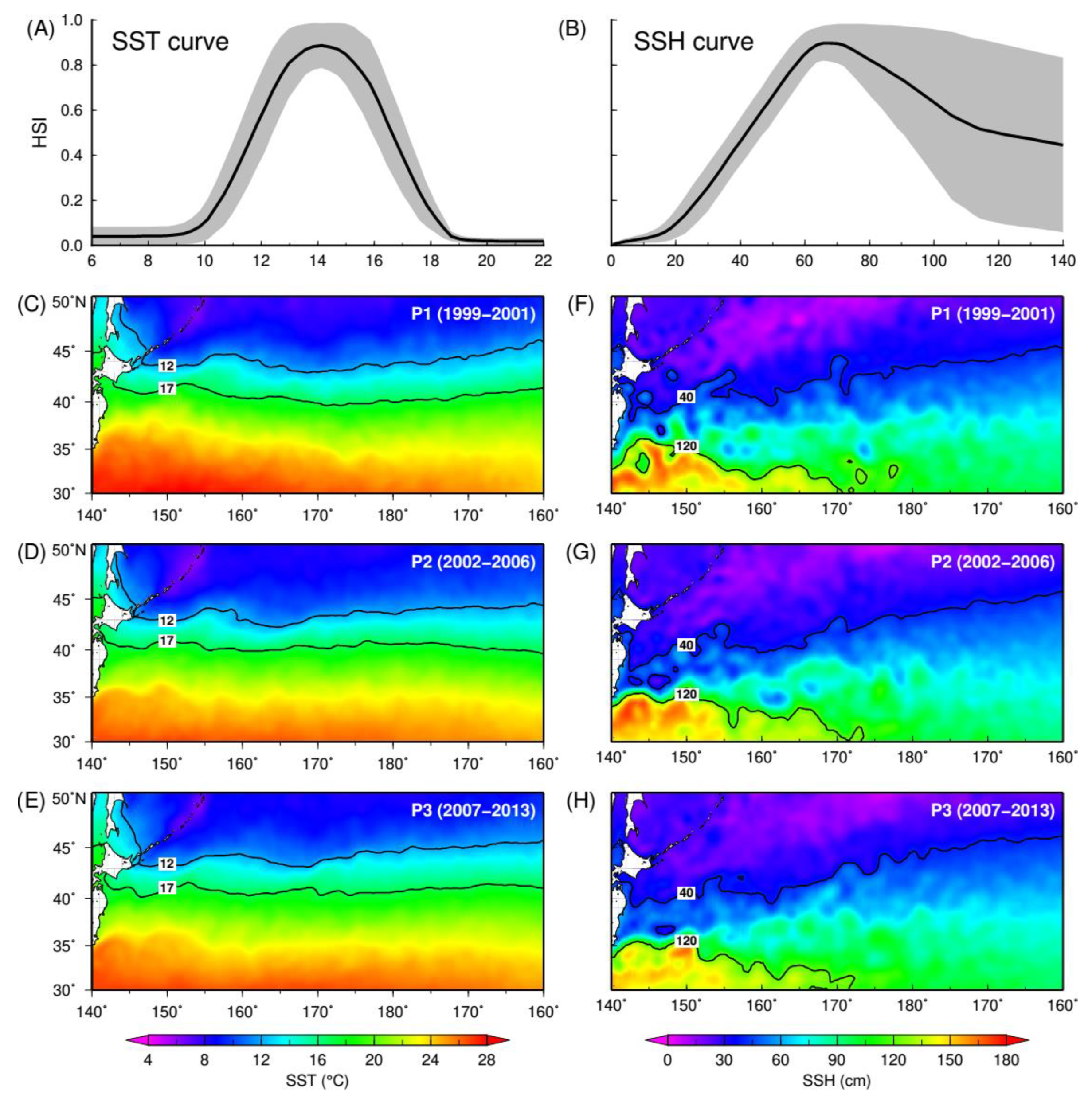
3.1. Squid Environmental Preferences

Preferred environmental ranges defining potential squid habitat were obtained from the multi-model simulations (from the best performing single-algorithm models; Table 2) and response curves for each of the environmental factors are shown in Figure 4A,B. The thermal conditions and mesoscale environment of squid habitat (HSI ≥ 0.5) were situated within the SST (Figure 4A) and SSH (Figure 4B) ranges from 12–17 °C and 40–120 cm, respectively. Period-specific spatial extents of optimal isotherms (Figure 4C–E) showed northward advance under the cold PDO phases (P1 and P3; Figure 4C,E) relative to its alternate phase (P2; Figure 4D). In contrast, the optimal isolines for SSH showed minimal differences in their geographic extent across PDO periods (Figure 4F–H). Nonetheless, the total area of pixels within the optimal SST and SSH limits was higher in the cold than in warm PDO phases (Table 4).

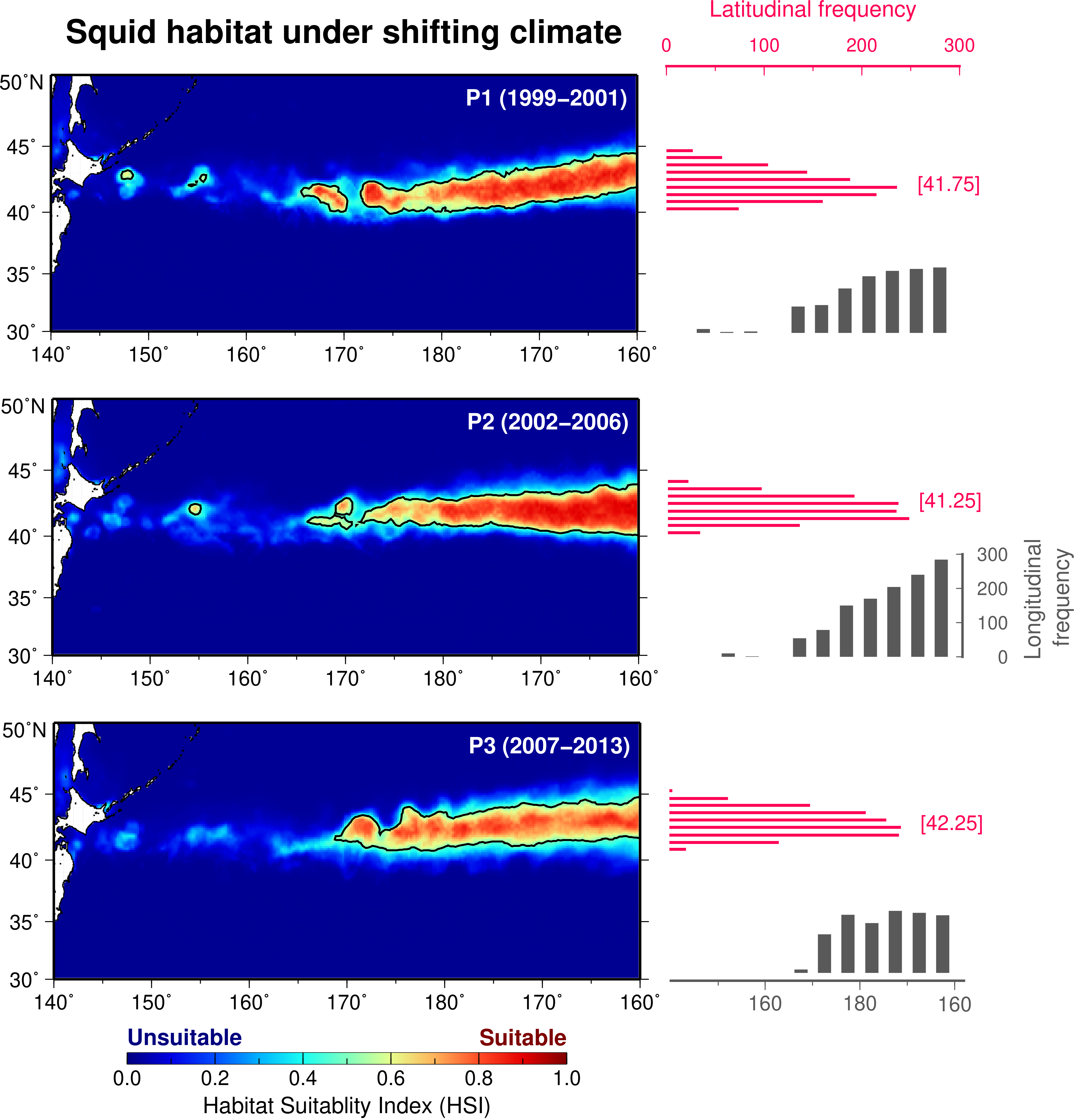
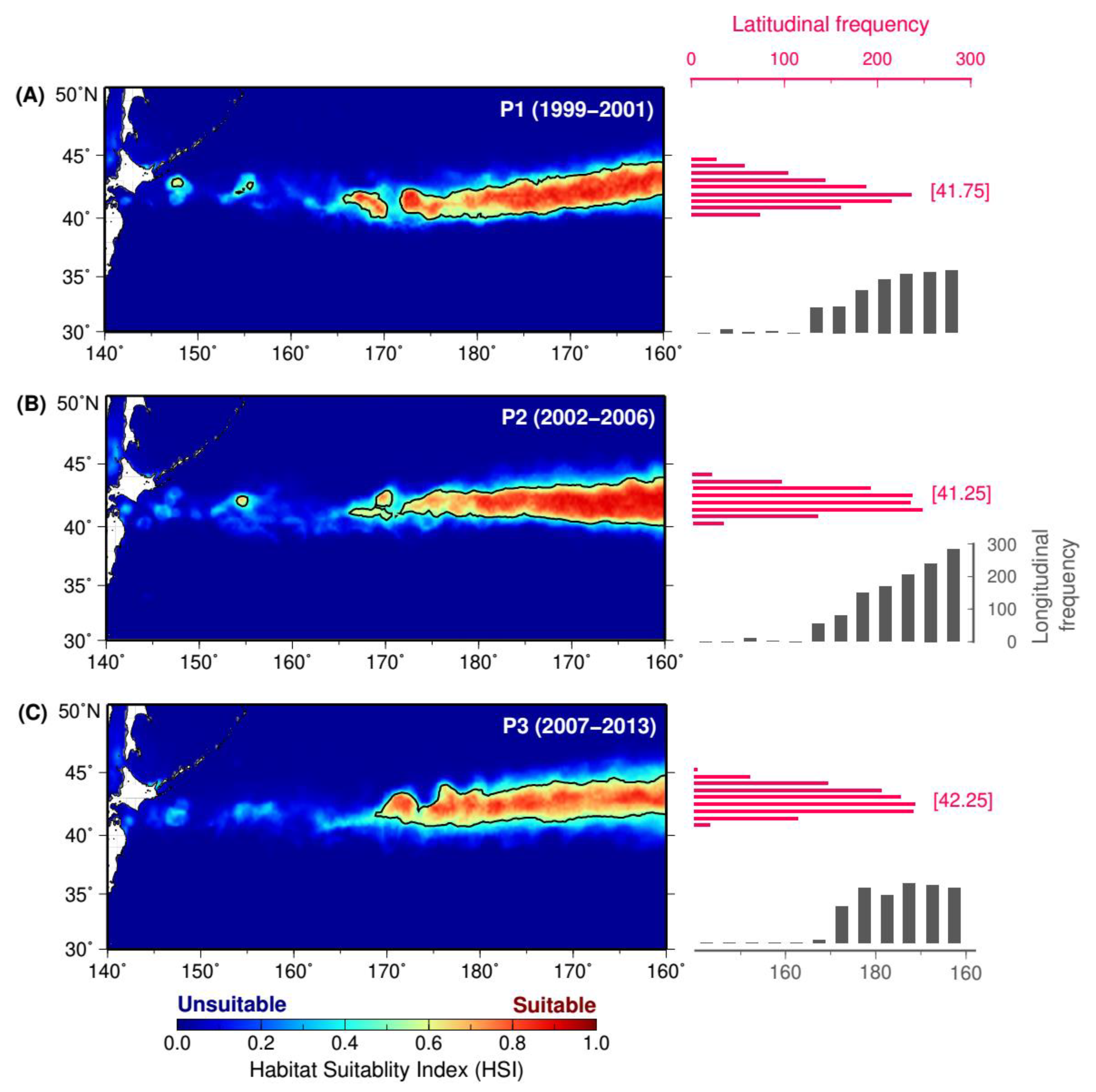
3.2. Spatial Patterns of Period-Specific Squid Habitat Forecasts

Potential squid habitat predictions obtained from the multi-model habitat ensemble highlighted differences in spatial distribution across PDO periods (Figure 5A–C, left panels). In particular, periods of cold PDO phases covered slightly broader, albeit patchy zones (Figure 5A,C left panels) of potential squid habitat relative to those predicted during the warm PDO phase (Figure 5B, left panel). Moreover, the zonal and meridional HSI frequencies (Figure 5A–C, right panels) further showed a northward advance of habitat suitability frequency peaks by as much as 1°N (~110 km) between the cold (P1 and P3) and warm (P2) PDO phases. Zonal pattern-wise, the frequency peak of habitat suitability also revealed a westward displacement in the latter period, concomitant with a spatial reduction in the total potential squid habitat area (Table 5).

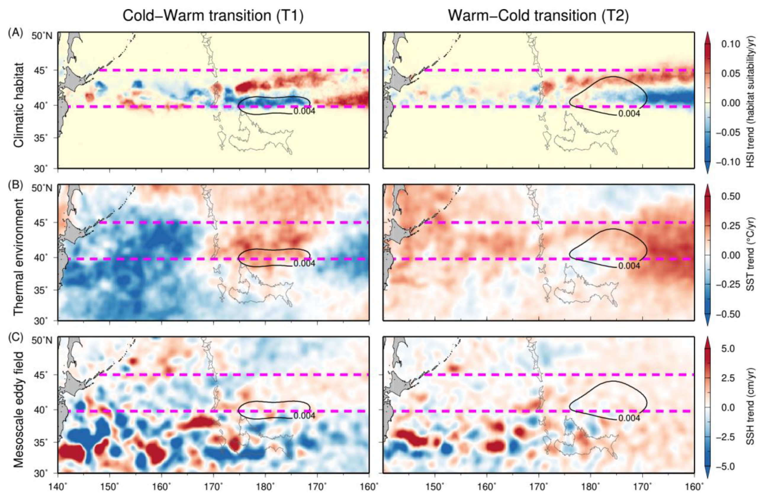
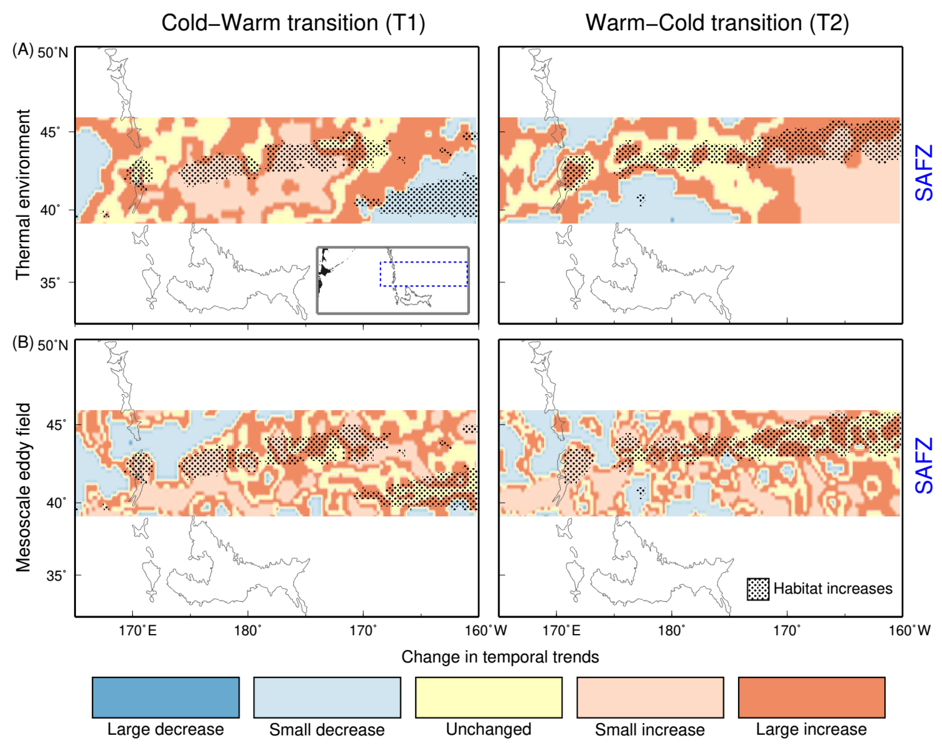
3.3. Temporal Trends in Squid Habitat and Environmental Conditions

Spatial distributions of temporal trends computed across contrasting PDO phase transitions for potential squid habitat and oceanographic conditions are shown in Figure 6A–C. Salient changes in trend patterns of potential squid habitat suitability emerged between the two phase transitions (Figure 6A). Highest rates of habitat loss (negative trend) and gain (positive trend) were located at the southern edge and northern part of the subarctic frontal zone (SAFZ, 40–45°N), respectively. In particular, during the first transition (T1; 1999–2006), positive trends in squid habitat suitability (0.03 ± 0.02 HSI/yr; mean annual rate ± 1 standard deviation) were observed along the northern part between 172°E–170°W and southeastern edge between 170–160°W of the SAFZ (Figure 6A, left panel). However, squid habitat losses were particularly pronounced at the southern border of the SAFZ between 162°E and 172°W (−0.04 ± 0.02 HSI/yr), further coinciding with the highest spatial density of the squid-fishing effort. During the second transition (T2; 2002–2013), the largest signal of habitat decline (−0.05 ± 0.03 HSI/yr) shifted east between 170° and 160°W (Figure 6A, right panel), with an average trend significantly higher than T1 (p < 0.001; unpaired t-test). Areas with positive HSI trend expanded east of the SAFZ, generating a continuous zone of squid habitat accretion. While the zonal extent of high squid fishing effort density remained considerably constant between the two transitions, squid fishing activity during T2 exhibited meridional expansion towards the northern fringe of the SAFZ (43–45°N). This concomitant spatial change in squid-fishing pattern suggested that squid jigging fleets were tracking the captured north-directed shifts in potential squid habitat quite reasonably during this climate phase transition.
Temporal trends in thermal and mesoscale environment similarly showed pronounced meridional and zonal patterns (Figure 6B,C). For instance, the latitudinal patterns in temporal trend for SST showed an extensive cooling signal (−0.07 ± 0.17 °C/yr) during the first transition (T1), further flanking a warming water parcel situated between 170°W and 170°E (Figure 6B, left panel). During the second transition (T2), however, thermal trend reversed toward a general warming pattern (0.09 ± 0.09 °C/yr), with highest warming rate east of the basin (175°–160°W; Figure 6B, right panel). Moreover, temporal SSH trends also revealed characteristic spatial patterns, capturing the ambient mesoscale environment at each climatic transition. For instance, meridional patterns showed consistent elevated temporal SSH trends between 175°E–160°W and within the latitudinal boundaries of SAFZ (40–45°N) across all transitions (Figure 6C, left and right panels). Overall, the mesoscale environment in the west and central North Pacific (140°E–160°W and 30–50°N) was characterized by the distinct overturn from cold-core (−0.39 ± 2.00 cm/yr) to warm-core (0.22 ± 1.08 cm/yr) dominated eddy field during the first (T1) and second (T2) transition, respectively.
Furthermore, the examination of temporal trends in potential squid habitat and oceanographic environment across PDO phase transitions showed salient spatial patterns, possibly regulating the transition-specific habitat responses. In general, the zonal habitat shifts showed differences in relative importance of the thermal and mesoscale forcing under contrasting PDO transitions. In particular, changes in habitat trends in the central (162°E–172°W; 40–44°N) North Pacific were likely modulated by transition-specific changes in both mesoscale and thermal conditions. Contrariwise, in the eastern North Pacific (170–160°W; 40–43°N), habitat trend changes appears to be responding more to thermal cues than mesoscale forcing. However, areas of increasing habitat irrespective of climatic transition have also been identified close to topographic features (i.e. emperor seamount chain) and northern part of the quasi-permanent temperate frontal zone (170°E–160°W; 43–45°N; SAFZ).
Further classification of the spatial overlap of regions classified with small and large increases in potential squid habitat with categorized changes in temporal trends of SST (Figure 7A) and SSH (Figure 7B) across phase transitions, showed that, indeed, areas sitting atop or close to the Emperor seamounts exhibited persistent habitat increases regardless of the PDO transition. Similarly, the patches of squid habitat increases proximal to the northern part of SAFZ (175°E–170°W; 43–45°N) were characterized by small increases to largely unchanged trends in thermal environment (Figure 7A) and mesoscale eddy field (Figure 7B) across the PDO phase transitions (left and right panels).

4. Discussion

While there are quite a vast number of studies looking at the patterns of suitable habitats for neon flying squid using the species distribution modeling approach [22,43,44,45], the framework of analyses implemented in the present study provided both qualitative and quantitative means of elucidating the effects of the dominant modes of climatic variability in the North Pacific Ocean at a decadal time-scale. Our results underpinned the differences in the temporal trends for suitable squid habitat across climatic transitions and, more importantly, afforded a quantitative estimate of the spatial changes in the squid habitat suitability over time. This allowed the characterization of sites that were particularly exposed and vulnerable to climatic oscillations while highlighting climate-resilient zones, exhibiting minimal changes in physical oceanographic properties over time.
Previous studies have described the spatial and temporal patterns of potential habitat of neon flying squid in response to dominant modes of high-frequency climate variability such as the El Niño Southern Oscillation (ENSO) [6,46,47]. Moreover, the impacts of the basin-wide regime shifts based on PDO patterns on relative abundances of autumn [7,8] and winter [35] cohorts of neon flying squid in the northwestern Pacific have been previously explored. Our analyses, however, focused on temporal habitat and environmental gradients in summer foraging zones of the autumn cohort (central Pacific; 160°W–160°E) under the contemporary PDO phase transitions, hence, affording insights into its distributional response to shifting climate and setting this work apart from previous studies. While the cold PDO phases (P1 and P3) revealed almost similar spatial extents of potential feeding habitats relative to the warm phase (P2), the averaged magnitude of squid habitat suitability was significantly higher in the latter (Table 3; p < 0.001; unpaired t-test). Such spatial and temporal patterns in potential squid habitat were likely modulated by the contrast in temporal trends in thermal and mesoscale features across a given PDO transition. Our previous analyses have shown a strong association of squid to warm-core eddies as important foraging features [22,23]. Henceforth, the prevalence of cold-core mesoscale circulation during T1 (Figure 6C, left panel) potentially explains the decline in the squid habitat around the south margin of the SAFZ. Similarly, our results reinforced earlier findings on the important roles of bathymetric and non-transient frontal structures in creating local, yet persistent, zones of climate-resilient foraging grounds for migratory taxa in the western and central North Pacific Ocean [23,48]. For instance, in oceanic environments where climatic parameters often exhibit minimal variability over wide spatial extents, the presence of topographic features can decouple climatic processes at local scales from basin-wide conditions [26,29]. In fact, this appears to be the case in our study area, as shown by an increasing squid habitat suitability trends (habitat gain) in waters proximal to seafloor features and temperate frontal zone, regardless of the climate transition (Figure 6A, left and right panels; Figure 7A,B). This suggests the potential of these sites as local refugia for squid and other pelagic resources [49,50] under changing environmental and climatic conditions in the open waters of the North Pacific Ocean.
In contrast, the climate-driven spatial potential habitat shifts across PDO phase transitions were particularly high between 39° and 47°N, with notable temporal trend reversal along the east–west direction. These results highlight and reassert the spatially-complex squid habitat responses not only to high-frequency modes of climate oscillation, but to low-frequency climate variability in the central and western North Pacific as well. In general, PDO impacts the basin-wide circulation patterns in the North Pacific basin, and ensuing changes in ocean currents have consequences on the heat, material and nutrient transport [51] which, in turn, could modulate the rates of biological production [52]. Further, zonal habitat shifts in the area within 162°E–172°W and 40–44°N suggest that these regions are most exposed to climate-driven changes in both thermal and mesoscale environments; thus, are potentially vulnerable to these impacts. The circulation dynamics in the transition zone (140°E–180; 35–40°N) between major frontal zones (i.e., sub-tropical and subarctic fronts) are highly variable due to the convergence of cold (Oyashio) and warm (Kuroshio) boundary currents [53,54]. The associated mesoscale eddies and flow instabilities that propagate northwestward of 40°N generate productive, albeit ephemeral feeding zones for numerous pelagic species [55,56,57]. In this region, the increasing trends in squid habitat during a mesoscale environment dominated by warm-core eddies (T2) suggest the higher affinity of squid to these features relative to the otherwise more productive cold-core rings. A similar response was recently observed from the tagging experiment of pelagic shark species in the Gulf Stream region [58]. The results from this work suggest that sharks use the core of anticyclonic ocean eddies as channels to forage at depths otherwise, unreachable due to the thermal physiological constraints. This could explain the reported affinity of neon flying squid (this study) and tuna species [55] to warm-core eddies in the pelagic waters of the Kuroshio region.
Moreover, in the temperate frontal zone (SAFZ; 170°E–160°W and 43–45°N), a region of increasing habitat suitability concurrent with warming waters were observed across all PDO phase transitions. In this area, the transition zone chlorophyll-a (TZCF) front were shown to assume its northernmost position during summer within our study region [6,23]. The TCZF is a permanent gradient in the sea surface color, persisting zonally across the North Pacific basin, with high and low chlorophyll to the north and south of the front, respectively [59,60]. Studies have suggested that this frontal feature could be important as a forage and migration habitat for pelagic species [61]. In the present analyses, periods of the extensive and sustained warming in these areas across the PDO phase transitions were likely to augment the potential squid habitat. This is particularly so, as the thermal conditions could become physiologically favorable (i.e., within the species’ thermal tolerance), allowing the squid to move further north and closer to the boundary of the TCZF. This similar distributional response of neon flying squid to elevated temperature in the central North Pacific was also noted earlier [6,47].
Finally, the analyses implemented in this work offered, to some extent, insights that substantiate the growing consensus on the significant effects of environmental and climatic variability on species habitat distributions across the marine and aquatic systems [62,63,64,65]. These impacts have important consequences, in terms of ecosystem functioning and provision of its services [66]. Furthermore, the rapidly accelerating pace of climate change warrants the exploration of means to monitor its ecological effects (e.g., using biological sentinels) [67] and consequently to create conservation and adaptation strategies (e.g., establishment of climate-smart protected areas and identification of potential climate refugia) [26,68]. Here, we have explored these aspects briefly, nonetheless, it is worth noting that our present analyses are subject to potential caveats and highlight areas of future research that can be done to reinforce our current findings. These caveats stem largely from the limited temporal span of available data (i.e., species occurrence records) that allow the robust detection of long-term trends in climate oscillations (basin-wide climate teleconnections, e.g., PDO) and resulting climate-driven ecological impacts. Thus, future work should aim at addressing these key issues through the incorporation of more recent data when made available.

5. Conclusions

Climate is a major driver in the spatial redistribution of marine species through its effects on the environment and on species’ optimal habitat. In the North Pacific, apart from high-frequency modes of climate oscillations, the low-frequency decadal-scale climate variability such as PDO significantly impacts the summer pelagic habitat of large oceanic squid. The effects ensued from the basin-wide changes in the ocean temperature and circulation, which in turn alters the foraging conditions for squid and translates to spatial shifts in the distribution of its potential habitat. Furthermore, the squid’s distributional responses exhibited zonal and meridional patterns, highlighting the relative sensitivity and exposure of certain areas to climate-modulated changes. The emergence of squid habitat patches and persistent zones of increasing habitat suitability across the PDO phase transitions (Figure 7A,B) underpins the importance of these sites as potential local climate refugia under anticipated threats of abruptly transpiring climate-driven environmental changes.

Author Contributions

I.D.A. and S.-I.S. conceived the idea for this study; H.I. and Y.I. (Yutaka Imamura) prepared and provided the squid fishery data used for analyses; S.-I.S., Y.I. (Yoichi Ishikawa) and H.I. contributed in the early discussions and framework design; I.D.A. wrote the paper with inputs from all of the authors. All authors have read and agreed to the published version of the manuscript.

Funding

This research was funded by Japan’s Research Program on Climate Change Adaptation (RECCA).

Acknowledgments

We thank the Research Program on Climate Change Adaptation (RECCA) of the Grant-in-Aid from Japan’s Ministry of Education, Culture, Sports, Science and Technology (MEXT) and Arctic Research Center, Hokkaido University for supporting this work. We are also extending our thanks to Aomori Prefectural Industrial Technology Research Center and the different research agencies for providing the data used in the analyses.

Conflicts of Interest

The authors declare no conflict of interest.

References

  1. Roper, C.F.E.; Sweeney, M.; Nauen, C. Cephalopods of the World, an Annotated and illustrated Catalogue of Species of Interest to Fisheries; FAO Fish Finder: Rome, Italy, 1984; Volume 3, pp. 1–277. [Google Scholar]
  2. Ichii, T.; Mahapatra, K.; Okamura, H.; Okada, Y. Stock assessment of the autumn cohort of neon flying squid (Ommastrephes bartramii) in the north pacific based on past large-scale high seas driftnet fishery data. Fish. Res. 2006, 78, 286–297. [Google Scholar] [CrossRef]
  3. Chen, X.; Liu, B.; Chen, Y. A review of the development of Chinese distant-water squid jigging fisheries. Fish. Res. 2008, 89, 211–221. [Google Scholar] [CrossRef]
  4. Arkhipkin, A.I.; Rodhouse, P.G.K.; Pierce, G.J.; Sauer, W.; Sakai, M.; Allcock, L.; Arguelles, J.; Bower, J.R.; Castillo, G.; Ceriola, L.; et al. World squid fisheries. Rev. Fish. Sci. Aquac. 2015, 23, 92–252. [Google Scholar] [CrossRef] [Green Version]
  5. Yatsu, A.; Midorikawa, S.; Shimada, T.; Uozumi, Y. Age and growth of the neon flying squid, Ommastrephes bartrami, in the North Pacific Ocean. Fish. Res. 1997, 29, 257–270. [Google Scholar] [CrossRef]
  6. Alabia, I.D.; Saitoh, S.-I.; Hirawake, T.; Igarashi, H.; Ishikawa, Y.; Usui, N.; Kamachi, M.; Awaji, T.; Seito, M. Elucidating the potential squid habitat responses in the central North Pacific to the recent ENSO flavors. Hydrobiologia 2016, 772, 1–13. [Google Scholar] [CrossRef]
  7. Ichii, T.; Mahapatra, K.; Sakai, M.; Wakabayashi, T.; Okamura, H.; Igarashi, H.; Inagake, D.; Okada, Y. Changes in abundance of the neon flying squid Ommastrephes bartramii in relation to climate change in the central North Pacific Ocean. Mar. Ecol. Prog. Ser. 2011, 441, 151–164. [Google Scholar] [CrossRef] [Green Version]
  8. Igarashi, H.; Ichii, T.; Sakai, M.; Ishikawa, Y.; Toyoda, T.; Masuda, S.; Sugiura, N.; Mahapatra, K.; Awaji, T. Possible link between interannual variation of neon flying squid (Ommastrephes bartramii) abundance in the North Pacific and the climate phase shift in 1998/1999. Prog. Oceanogr. 2017, 150, 20–34. [Google Scholar] [CrossRef]
  9. Ichii, T.; Mahapatra, K.; Sakai, M.; Okada, Y. Life history of the neon flying squid: Effect of the oceanographic regime in the North Pacific Ocean. Mar. Ecol. Prog. Ser. 2009, 378, 1–11. [Google Scholar] [CrossRef]
  10. Doubleday, Z.A.; Prowse, T.A.A.; Arkhipkin, A.; Pierce, G.J.; Semmens, J.; Steer, M.; Leporati, S.C.; Lourenço, S.; Quetglas, A.; Sauer, W.; et al. Global proliferation of cephalopods. Curr. Biol. 2016, 26, R406–R407. [Google Scholar] [CrossRef] [Green Version]
  11. Bower, J.R.; Ichii, T. The red flying squid (Ommastrephes bartramii): A review of recent research and the fishery in Japan. Fish. Res. 2005, 76, 39–55. [Google Scholar] [CrossRef]
  12. Parry, M. Feeding behavior of two ommastrephid squids Ommastrephes bartramii and Sthenoteuthis oualaniensis off Hawaii. Mar. Ecol. Prog. Ser. 2006, 318, 229–235. [Google Scholar] [CrossRef]
  13. Watanabe, H.; Kubodera, T.; Ichii, T.; Kawahara, S. Feeding habits of neon flying squid Ommastrephes bartramii in the transitional region of the central North Pacific. Mar. Ecol. Prog. Ser. 2004, 266, 173–184. [Google Scholar] [CrossRef] [Green Version]
  14. Bates, A.E.; Pecl, G.T.; Frusher, S.; Hobday, A.J.; Wernberg, T.; Smale, D.A.; Sunday, J.M.; Hill, N.A.; Dulvy, N.K.; Colwell, R.K.; et al. Defining and observing stages of climate-mediated range shifts in marine systems. Glob. Environ. Chang. 2014, 26, 27–38. [Google Scholar] [CrossRef]
  15. Gunderson, A.R.; Armstrong, E.J.; Stillman, J.H. Multiple stressors in a changing world: The need for an improved perspective on physiological responses to the dynamic marine environment. Annu. Rev. Mar. Sci. 2016, 8, 357–378. [Google Scholar] [CrossRef]
  16. Salinger, M.J.; Bell, J.D.; Evans, K.; Hobday, A.J.; Allain, V.; Brander, K.; Dexter, P.; Harrison, D.E.; Hollowed, A.B.; Lee, B.; et al. Climate and oceanic fisheries: Recent observations and projections and future needs. Clim. Chang. 2013, 119, 213–221. [Google Scholar] [CrossRef]
  17. Anderson, C.I.H.; Rodhouse, P.G. Life cycles, oceanography and variability: Ommastrephid squid in variable oceanographic environments. Fish. Res. 2001, 54, 133–143. [Google Scholar] [CrossRef]
  18. Rodhouse, P.G. Managing and forecasting squid fisheries in variable environments. Fish. Res. 2001, 54, 3–8. [Google Scholar] [CrossRef]
  19. Abrahms, B.; Welch, H.; Brodie, S.; Jacox, M.G.; Becker, E.A.; Bograd, S.J.; Irvine, L.M.; Palacios, D.M.; Mate, B.R.; Hazen, E.L. Dynamic ensemble models to predict distributions and anthropogenic risk exposure for highly mobile species. Divers. Distrib. 2019, 25, 1182–1193. [Google Scholar] [CrossRef] [Green Version]
  20. Burgeot, T.; Akcha, F.; Ménard, D.; Robinson, C.; Loizeau, V.; Brach-Papa, C.; Martínez-Gòmez, C.; Le Goff, J.; Budzinski, H.; Le Menach, K.; et al. Integrated monitoring of chemicals and their effects on four sentinel species, Limanda limanda, Platichthys flesus, Nucella lapillus and Mytilus sp., in Seine Bay: A key step towards applying biological effects to monitoring. Mar. Environ. Res. 2017, 124, 92–105. [Google Scholar] [CrossRef] [Green Version]
  21. Fossi, M.C.; Panti, C.; Baini, M.; Lavers, J.L. A review of plastic-associated pressures: Cetaceans of the mediterranean sea and eastern australian shearwaters as case studies. Front. Mar. Sci. 2018, 5, 173. [Google Scholar] [CrossRef]
  22. Alabia, I.D.; Saitoh, S.-I.; Mugo, R.; Igarashi, H.; Ishikawa, Y.; Usui, N.; Kamachi, M.; Awaji, T.; Seito, M. Seasonal potential fishing ground prediction of neon flying squid (Ommastrephes bartramii) in the western and central North Pacific. Fish. Oceanogr. 2015, 24, 190–203. [Google Scholar] [CrossRef]
  23. Alabia, I.D.; Saitoh, S.-I.; Mugo, R.; Igarashi, H.; Ishikawa, Y.; Usui, N.; Kamachi, M.; Awaji, T.; Seito, M. Identifying pelagic habitat hotspots of neon flying squid in the temperate waters of the central North Pacific. PLoS ONE 2015, 10, e0142885. [Google Scholar] [CrossRef] [Green Version]
  24. Keppel, G.; Van Niel, K.P.; Wardell-Johnson, G.W.; Yates, C.J.; Byrne, M.; Mucina, L.; Schut, A.G.T.; Hopper, S.D.; Franklin, S.E. Refugia: Identifying and understanding safe havens for biodiversity under climate change. Glob. Ecol. Biogeogr. 2012, 21, 393–404. [Google Scholar] [CrossRef]
  25. Ashcroft, M.B. Identifying refugia from climate change. J. Biogeogr. 2010, 37, 1407–1413. [Google Scholar] [CrossRef]
  26. Ban, S.S.; Alidina, H.M.; Okey, T.A.; Gregg, R.M.; Ban, N.C. Identifying potential marine climate change refugia: A case study in Canada’s Pacific marine ecosystems. Glob. Ecol. Conserv. 2016, 8, 41–54. [Google Scholar] [CrossRef] [Green Version]
  27. Clark, M.R.; Schlacher, T.A.; Rowden, A.A.; Stocks, K.I.; Consalvey, M. Science priorities for seamounts: Research links to conservation and management. PLoS ONE 2012, 7, e29232. [Google Scholar] [CrossRef] [Green Version]
  28. Scales, K.L.; Miller, P.I.; Hawkes, L.A.; Ingram, S.N.; Sims, D.W.; Votier, S.C. Review: On the front line: Frontal zones as priority at-sea conservation areas for mobile marine vertebrates. J. Appl. Ecol. 2014, 51, 1575–1583. [Google Scholar] [CrossRef] [Green Version]
  29. Morato, T.; Hoyle, S.D.; Allain, V.; Nicol, S.J. Seamounts are hotspots of pelagic biodiversity in the open ocean. Proc. Natl. Acad. Sci. USA 2010, 107, 9707–9711. [Google Scholar] [CrossRef] [Green Version]
  30. Mantua, N.J.; Hare, S.R.; Zhang, Y.; Wallace, J.M.; Francis, R.C. A Pacific interdecadal climate oscillation with impacts on salmon production. Bull. Am. Meteorol. Soc. 1997, 78, 1069–1079. [Google Scholar] [CrossRef]
  31. Newman, M.; Alexander, M.A.; Ault, T.R.; Cobb, K.M.; Deser, C.; Di Lorenzo, E.; Mantua, N.J.; Miller, A.J.; Minobe, S.; Nakamura, H.; et al. The Pacific Decadal Oscillation, revisited. J. Clim. 2016, 29, 4399–4427. [Google Scholar] [CrossRef] [Green Version]
  32. Zwolinski, J.P.; Demer, D.A. Environmental and parental control of Pacific sardine (Sardinops sagax) recruitment. ICES J. Mar. Sci. 2014, 71, 2198–2207. [Google Scholar] [CrossRef] [Green Version]
  33. Litzow, M.A.; Ciannelli, L.; Puerta, P.; Wettstein, J.J.; Rykaczewski, R.R.; Opiekun, M. Non-stationary climate–salmon relationships in the Gulf of Alaska. Proceed. R. Soc. B Biol. Sci. 2018, 285, 20181855. [Google Scholar] [CrossRef] [PubMed] [Green Version]
  34. Mantua, N.J.; Hare, S.R. The Pacific Decadal Oscillation. J. Oceanogr. 2002, 58, 35–44. [Google Scholar] [CrossRef]
  35. Yu, W.; Chen, X.; Yi, Q.; Chen, Y. Influence of oceanic climate variability on stock level of western winter–spring cohort of Ommastrephes bartramii in the northwest Pacific Ocean. Int. J. Remote Sens. 2016, 37, 3974–3994. [Google Scholar] [CrossRef]
  36. Wessel, P.; Smith, W.H.F.; Scharroo, R.; Luis, J.; Wobbe, F. Generic mapping tools: Improved version released. Eos Trans. Am. Geophys. Union 2013, 94, 409–410. [Google Scholar] [CrossRef] [Green Version]
  37. Thuiller, W.; Georges, D.; Engler, R.; Breiner, F. Biomod2: Ensemble Platform for Species Distribution Modeling. R Package Version 3.3-7. 2016. Available online: http://CRAN.R-project.org/package=biomod2 (accessed on 10 January 2016).
  38. Barbet-Massin, M.; Jiguet, F.; Albert, C.H.; Thuiller, W. Selecting pseudo-absences for species distribution models: How, where and how many? Methods Ecol. Evol. 2012, 3, 327–338. [Google Scholar] [CrossRef]
  39. Alabia, I.D.; Saitoh, S.-I.; Igarashi, H.; Ishikawa, Y.; Usui, N.; Kamachi, M.; Awaji, T.; Seito, M. Ensemble squid habitat model using three-dimensional ocean data. ICES J. Mar. Sci. 2016, 73, 1863–1874. [Google Scholar] [CrossRef] [Green Version]
  40. Scales, K.L.; Miller, P.I.; Ingram, S.N.; Hazen, E.L.; Bograd, S.J.; Phillips, R.A. Identifying predictable foraging habitats for a wide-ranging marine predator using ensemble ecological niche models. Divers. Distrib. 2016, 22, 212–224. [Google Scholar] [CrossRef] [Green Version]
  41. Allouche, O.; Tsoar, A.; Kadmon, R. Assessing the accuracy of species distribution models: Prevalence, kappa and the true skill statistic (tss). J. Appl. Ecol. 2006, 43, 1223–1232. [Google Scholar] [CrossRef]
  42. R Core Team. R: A Language and Environment for Statistical Computing; R Foundation for Statistical Computing: Vienna, Austria, 2019. [Google Scholar]
  43. Chen, X.; Tian, S.; Chen, Y.; Liu, B. A modeling approach to identify optimal habitat and suitable fishing grounds for neon flying squid (Ommastrephes bartramii) in the northwest Pacific Ocean. Fish. Bull. 2010, 108, 14. [Google Scholar]
  44. Igarashi, H.; Ishikawa, Y.; Nishikawa, H.; Usui, N.; Sakai, M.; Saitoh, S.I.; Imamura, Y. Habitat Suitability Index Model for Neon Flying Squid Adding Its Stock Effect; Techno-Ocean: Kobe, Japan, 2016; pp. 449–453. [Google Scholar]
  45. Igarashi, H.; Saitoh, S.-I.; Ishikawa, Y.; Kamachi, M.; Usui, N.; Sakai, M.; Imamura, Y. Identifying potential habitat distribution of the neon flying squid (Ommastrephes bartramii) off the eastern coast of Japan in winter. Fish. Oceanogr. 2018, 27, 16–27. [Google Scholar] [CrossRef]
  46. Chen, X.J.; Zhao, X.H.; Chen, Y. Influence of el niño/la niña on the western winter–spring cohort of neon flying squid (Ommastrephes bartramii) in the northwestern pacific ocean. ICES J. Mar. Sci. 2007, 64, 1152–1160. [Google Scholar] [CrossRef] [Green Version]
  47. Yu, W.; Chen, X.; Yi, Q.; Chen, Y.; Zhang, Y. Variability of suitable habitat of western winter-spring cohort for neon flying squid in the northwest Pacific under anomalous environments. PLoS ONE 2015, 10, e0122997. [Google Scholar] [CrossRef] [PubMed] [Green Version]
  48. Kai, M.; Thorson, J.T.; Piner, K.R.; Maunder, M.N. Predicting the spatio-temporal distributions of pelagic sharks in the western and central North Pacific. Fish. Oceanogr. 2017, 26, 569–582. [Google Scholar] [CrossRef]
  49. Morato, T.; Hoyle, S.D.; Allain, V.; Nicol, S.J. Tuna longline fishing around west and central pacific seamounts. PLoS ONE 2011, 5, e14453. [Google Scholar] [CrossRef] [PubMed]
  50. Morato, T.; Varkey, D.A.; Damaso, C.; Machete, M.; Santos, M.; Prieto, R.; Pitcher, T.J.; Santos, R.S. Evidence of a seamount effect on aggregating visitors. Mar. Ecol. Prog. Ser. 2008, 357, 23–32. [Google Scholar] [CrossRef]
  51. Chiba, S.; Di Lorenzo, E.; Davis, A.; Keister, J.E.; Taguchi, B.; Sasai, Y.; Sugisaki, H. Large-scale climate control of zooplankton transport and biogeography in the Kuroshio-Oyashio extension region. Geophys. Res. Lett. 2013, 40, 5182–5187. [Google Scholar] [CrossRef]
  52. Macias, D.; Landry, M.R.; Gershunov, A.; Miller, A.J.; Franks, P.J.S. Climatic control of upwelling variability along the western north-american coast. PLoS ONE 2012, 7, e30436. [Google Scholar] [CrossRef] [Green Version]
  53. Chiba, S.; Sugisaki, H.; Nonaka, M.; Saino, T. Geographical shift of zooplankton communities and decadal dynamics of the Kuroshio–Oyashio currents in the western North Pacific. Glob. Chang. Biol. 2009, 15, 1846–1858. [Google Scholar] [CrossRef]
  54. Qiu, B.; Chen, S.; Schneider, N. Dynamical links between the decadal variability of the Oyashio and Kuroshio extensions. J. Clim. 2017, 30, 9591–9605. [Google Scholar] [CrossRef]
  55. Mugo, R.; Saitoh, S.-I.; Nihira, A.; Kuroyama, T. Habitat characteristics of skipjack tuna (Katsuwonus pelamis) in the western North Pacific: A remote sensing perspective. Fish. Oceanogr. 2010, 19, 382–396. [Google Scholar] [CrossRef]
  56. Zainuddin, M.; Kiyofuji, H.; Saitoh, K.; Saitoh, S.-I. Using multi-sensor satellite remote sensing and catch data to detect ocean hot spots for albacore (Thunnus alalunga) in the northwestern North Pacific. Deep Sea Res. Part II Top. Stud. Oceanogr. 2006, 53, 419–431. [Google Scholar] [CrossRef]
  57. Yatsu, A.; Chiba, S.; Yamanaka, Y.; Ito, S.-I.; Shimizu, Y.; Kaeriyama, M.; Watanabe, Y. Climate forcing and the Kuroshio/Oyashio ecosystem. ICES J. Mar. Sci. 2013, 70, 922–933. [Google Scholar] [CrossRef] [Green Version]
  58. Braun, C.D.; Gaube, P.; Sinclair-Taylor, T.H.; Skomal, G.B.; Thorrold, S.R. Mesoscale eddies release pelagic sharks from thermal constraints to foraging in the ocean twilight zone. Proc. Natl. Acad. Sci. USA 2019, 116, 17187. [Google Scholar] [CrossRef] [Green Version]
  59. Ayers, J.M.; Lozier, M.S. Physical controls on the seasonal migration of the North Pacific transition zone chlorophyll front. J. Geophys. Res. Oceans 2010, 115, 1–11. [Google Scholar] [CrossRef] [Green Version]
  60. Polovina, J.J.; Howell, E.; Kobayashi, D.R.; Seki, M.P. The transition zone chlorophyll front, a dynamic global feature defining migration and forage habitat for marine resources. Prog. Oceanogr. 2001, 49, 469–483. [Google Scholar] [CrossRef]
  61. Polovina, J.J.; Howell, E.A.; Kobayashi, D.R.; Seki, M.P. The transition zone chlorophyll front updated: Advances from a decade of research. Prog. Oceanogr. 2017, 150, 79–85. [Google Scholar] [CrossRef]
  62. Pecl, G.; Jackson, G. The potential impacts of climate change on inshore squid: Biology, ecology and fisheries. Rev. Fish. Biol. Fish. 2008, 18, 373–385. [Google Scholar] [CrossRef]
  63. Poloczanska, E.S.; Burrows, M.T.; Brown, C.J.; García Molinos, J.; Halpern, B.S.; Hoegh-Guldberg, O.; Kappel, C.V.; Moore, P.J.; Richardson, A.J.; Schoeman, D.S.; et al. Responses of marine organisms to climate change across oceans. Front. Mar. Sci. 2016, 3, 1–21. [Google Scholar] [CrossRef] [Green Version]
  64. Guraslan, C.; Fach, B.A.; Oguz, T. Understanding the impact of environmental variability on anchovy overwintering migration in the black sea and its implications for the fishing industry. Front. Mar. Sci. 2017, 4, 275. [Google Scholar] [CrossRef] [Green Version]
  65. Alabia, I.D.; García Molinos, J.; Saitoh, S.-I.; Hirawake, T.; Hirata, T.; Mueter, F.J. Distribution shifts of marine taxa in the Pacific Arctic under contemporary climate changes. Divers. Distrib. 2018, 24, 1583–1597. [Google Scholar] [CrossRef] [Green Version]
  66. Townsend, M.; Davies, K.; Hanley, N.; Hewitt, J.E.; Lundquist, C.J.; Lohrer, A.M. The challenge of implementing the marine ecosystem service concept. Front. Mar. Sci. 2018, 5, 359. [Google Scholar] [CrossRef] [Green Version]
  67. Hazen, E.L.; Abrahms, B.; Brodie, S.; Carroll, G.; Jacox, M.G.; Savoca, M.S.; Scales, K.L.; Sydeman, W.J.; Bograd, S.J. Marine top predators as climate and ecosystem sentinels. Front. Ecol. Environ. 2019, 17, 565–574. [Google Scholar] [CrossRef] [Green Version]
  68. Tittensor, D.P.; Beger, M.; Boerder, K.; Boyce, D.G.; Cavanagh, R.D.; Cosandey-Godin, A.; Crespo, G.O.; Dunn, D.C.; Ghiffary, W.; Grant, S.M.; et al. Integrating climate adaptation and biodiversity conservation in the global ocean. Sci. Adv. 2019, 5, 9969. [Google Scholar] [CrossRef] [Green Version]
Figure 1. (A) Map of the North Pacific, showing the study area enclosed by the dotted box. Further highlighted are the major oceanographic (currents and frontal zones) and topographic features, along with the putative geographical extents of the annual migration between the spawning and foraging grounds for the autumn cohort of the neon flying squid [7]. (B) Spatial distributions of Japanese squid fishing effort (expressed as the total number of fishing vessel per 0.25° geographic grid) in summers between May and July 1999–2013.
Remotesensing 12 00521 g001
Figure 2. (A) Annual-averaged index of Pacific decadal oscillation (PDO) used to identify the climatic periods, representing the cold (Period 1, P1: 1999–2001 and Period 3, P3: 2007–2013) and warm (Period 2, P2: 2002–2006) PDO phases. The climatic transitions were defined by the PDO phase shifts between consecutive periods (Transition 1, T1: 1999–2006 and Transition 2, T2: 2002–2013) (B) Spatial maps of sea surface temperature anomalies (SSTA) relative to the 15-year climatological average in the North Pacific for periods of distinct PDO climatic regime.
Remotesensing 12 00521 g002
Figure 3. Analytical framework used for the study. Multi-model ensemble were constructed to elucidate the summer potential squid habitat over a 15-year period, punctuated by distinct phase transitions of Pacific decadal oscillation (PDO). The magnitude and rate of spatial changes in the potential squid habitat and oceanographic conditions were quantified based on the temporal trends in the habitat suitability index (HSI), thermal environment (sea surface temperature; SST) and mesoscale circulation (sea surface height; SSH) across the climatic transitions from cold to warm (Transition 1, T1: 1999–2006) and warm to cold PDO phase shift (Transition 2, T2: 2002–2013).
Remotesensing 12 00521 g003
Figure 4. Multi-model squid habitat response curves for the (A) SST and (B) SSH, averaged from eight (8) single-algorithm models with the corresponding ±1 standard deviation (SD; gray shading). Spatial distributions of the summer-averaged (May–July) SST and SSH for the following periods, respectively: (C,F) P1 (1999–2001), (D,G) P2 (2002–2006), and (E,H) P3 (2007–2013). Overlain as solid lines are the model-derived optimal ranges for SST (12–17 °C) and SSH (40–120 cm) at each period.
Remotesensing 12 00521 g004
Figure 5. Spatial maps of potential squid habitat (left panels) with corresponding zonal (gray bars) and meridional (red bars) frequencies (right panels) for the following periods: (A) P1 (1999–2001), (B) P2 (2002–2006), and (C) P3 (2007–2013). Overlain on the spatial maps are contours delineating the regions with moderate to high squid habitat suitability (HSI ≥ 0.5). Latitudinal bin corresponding to the HSI frequency peaks for each period were also labeled (values in brackets).
Remotesensing 12 00521 g005
Figure 6. Spatial maps of the temporal trends computed for (A) potential squid habitat, (B) thermal environment, and (C) mesoscale eddy field, during the PDO phase transitions from a cold to warm (T1, left panels) and warm to cold (T2, right panels) phase. The spatial signals of the decrease and increase in the climatic habitat suitability, temperature and mesoscale activity for a given phase transition are represented by blue and red shades, respectively. The solid contours correspond to the highest spatial density of squid fishing effort for each climatic transition, gray polygons represent the topographic features and the region within the broken lines correspond to the spatial domain of the subarctic frontal zone (SAFZ).
Remotesensing 12 00521 g006
Figure 7. Maps showing the spatial overlap in regions of small and large increases in potential squid habitat (overlain dot-filled polygons) with the categorized temporal trend changes in the (A) thermal environment and (B) mesoscale eddy field, during the cold-warm (T1, left panels) and warm-cold (T2, right panels) PDO phase transitions. The subset area (subarctic frontal zone, SAFZ) corresponds to the dashed bordered polygon in the inset map. Seafloor features are also highlighted in solid gray lined polygons.
Remotesensing 12 00521 g007
Table 1. List of the species habitat models and the parametrization settings used to generate the summer potential squid habitat in the study area, available through the BIOMOD2 package version 3.3-7.
Model AlgorithmAbbrevModel Parameterization SettingsR Packages
Generalized linear modelGLMfamily = ‘binomial’ (link = ‘logit’), type = ‘quadratic’stats ver. 3.4.4
Generalized additive modelGAMfamily = ‘binomial’ (link = ‘logit’), type = ‘s_smoother’,mgcv ver. 1.8-23
Boosted Regression TreesGBMdistribution = ‘bernoulli’, number of trees = 2500, shrinkage = 0.001, bag fraction = 0.5, train fraction = 1, cross-validation folds = 3gbm ver. 2.1.3
Classification Tree AnalysisCTAmethod = class, complexity parameter = 0.001, cross-validation folds = 5 rpart ver. 4.1–13
Artificial Neural NetworkANNmaximum iteration = 200, cross-validation folds = 5, random weight = 0.1nnet ver. 7.3–12
Surface Range EnvelopSREtolerance boundary cut-off = 0.025biomod2 3.3–7
Flexible Discriminant AnalysisFDAregression method = ‘mars’biomod2 3.3–7
Multiple Adaptive Regression SplinesMARSmaximum interaction degree = 2, penalty = 2, forward stepwise stopping threshold = 0.001, prune feature enabled biomod2 3.3–7
Random ForestRFnumber of trees = 500, node size = 5biomod2 3.3–7
Maximum EntropyMaxEntmaximum training iterations = 200, linear/quadratic/product/hinge features enabled, default prevalence = 0.5MaxEnt ver. 3.4.0
Table 2. List of single-algorithm species distribution models used for mapping potential squid habitat distribution with the respective performance metrics obtained during the model runs. Based on the true skill statistics (TSS), multi-model ensemble was developed using models with TSS ≥ 0.80. Model algorithms in bold were excluded in the final ensemble habitat model as their TSS values were below the cut-off.
Species Distribution Models (SDMs)AbbreviationsModel Performance Metrics
AUCKappaTSS
Generalized additive modelGAM0.9520.6460.810
Generalized linear modelGLM0.9500.6440.803
Generalized boosting modelGBM0.9570.6590.822
Artificial neural networkANN0.9550.6540.814
Random forestRF0.9550.6510.810
Maximum entropyMaxEnt0.9540.6410.801
Classification tree analysisCTA0.9240.6370.807
Surface range envelopeSRE0.8880.6030.776
Flexible discriminant analysisFDA0.9450.6170.785
Multivariate adaptive regression splinesMARS0.9520.6480.810
Table 3. Computed quintiles for the temporal trends of potential habitat (HSI), thermal environment (SST) and mesoscale eddy field (SSH) for each PDO phase transition. The corresponding values were used to classify the variable-specific changes in the temporal trends.
PDO Phase TransitionsCategoriesLarge DecreaseSmall DecreaseLargely UnchangedSmall IncreaseLarge Increase
Variables (Unit)0%20%40%60%80%100%
Cold-Warm (T1)Habitat (HSI)−0.0928−0.0133−0.00020.00610.02900.1339
SST (°C/yr)−2.8460−0.58050.02520.33110.62112.9051
SSH (cm/yr)−0.3578−0.10930.02630.10420.18220.3739
Warm-Cold (T2)Habitat (HSI)−0.0943−0.01990.00000.00360.02400.0712
SST (°C/yr)−1.47250.09960.30720.44630.65373.0849
SSH (cm/yr)−0.09830.03880.09670.15690.23840.3722
Table 4. Preferred ranges for SST and SSH derived from the multi-model habitat ensemble, with the corresponding total area falling within these optimal environmental conditions for the neon flying squid under PDO-specific periods.
Environmental FactorsOptimal RangesTotal Area (1 × 10⁶ km2)
P1 (1999–2001)P2 (2002–2006)P3 (2007–2013)
SST12–17 °C1.961.851.98
SSH40–120 cm6.266.006.37
Table 5. Summary statistics of the spatial extent of inferred potential squid habitat across the different PDO periods. The total area with moderate to high potential squid habitat (HSI ≥ 0.5), overall habitat suitability (HSI) average and standard deviation (SD) were computed for each PDO-specific periods from 1999–2013.
PDO-Based Climatic PeriodsRanges (Minimum, Maximum)HSI Mean ± 1SDTotal Area
(1 × 10⁵ km2)
LongitudeLatitudeHSI
P1 (1999–2001)147.25, 200.0040.00, 44.500.50, 0.900.70 ± 0.116.93
P2 (2002–2006)154.00, 200.0040.00, 44.000.50, 0.920.72 ± 0.126.87
P3 (2007–2013)168.75, 200.0040.75, 44.750.50, 0.870.67 ± 0.097.01

