Abstract
Simplified models are widely applied in finite element computations regarding mechanical and structural problems. However, the simplified model sometimes causes many deviations in the finite element analysis (FEA) of structures, especially in the non-designed structures which have undergone unknowable deformation features. Hence, a novel FEA methodology based on the parametric model by approximating three-dimensional (3D) feature data is proposed to solve this problem in the present manuscript. Many significant and effective technologies have been developed to detect 3D feature information accurately, e.g., terrestrial laser scanning (TLS), digital photogrammetry, and radar technology. In this manuscript, the parametric FEA model combines 3D point clouds from TLS and the parametric surface approximation method to generate 3D surfaces and models accurately. TLS is a popular measurement method for reliable 3D point clouds acquisition and monitoring deformations of structures with high accuracy and precision. The B-spline method is applied to approximate the measured point clouds data automatically and generate a parametric description of the structure accurately. The final target is to reduce the effects of the model description and deviations of the FEA. Both static and dynamic computations regarding a composite structure are carried out by comparing the parametric and general simplified models. The comparison of the deformation and equivalent stress of future behaviors are reflected by different models. Results indicate that the parametric model based on the TLS data is superior in the finite element computation. Therefore, it is of great significance to apply the parametric model in the FEA to compute and predict the future behavior of the structures with unknowable deformations in engineering accurately.
1. Introduction
The present manuscript proposes a novel finite element analysis (FEA) methodology which is based on the accurate parametric surface model by fitting the actual three-dimensional (3D) feature data. 3D feature data can be detected by many efficient measurement methods, e.g., terrestrial laser scanning (TLS), digital photogrammetry, and radar technology. This parametric model is realized by approximating the point clouds data from TLS which is an accurate and real-time measurement method. The final goal is to improve the accuracy of finite element (FE) computation results due to geometric model errors, especially in the analysis of structures which have undergone unknowable deformation features.
1.1. Background
It is widely recognized today that FE methods permit the analysis of engineering systems to be increasingly accurate and intelligent. The influence of the computational uncertainties regarding the system behavior leads the scientific community to recognize the importance of accuracy in engineering application problems [1]. An accurate FE computation can improve the design efficiency and the reliability of the analysis and prediction in the actual engineering applications. Engineering experiences show that the accuracy problems do not only include the assessment of the material [2,3,4,5] but also the geometry model of the engineering structures [6]. The use of the geometric constitution has been verified in the field of the virtual modelling application [7,8].
Geometric simplifications generally have to be adapted in the FE computation process. Losses of geometric information and connection inconsistencies between numerical models and true objects are obvious during the simplification. Consequently, issues related to the geometric model generation and its accuracy in the computational models are continuously gaining significance [9]. The geometric accuracy and structural optimization are still highlights and challenging topics in the field of the FEA. Therefore, accurate and fast measurement technologies play important roles in the object acquisition and geometric description. This is a reasonable and feasible solution to improve the accuracy of the geometry in this FEA process.
1.2. Geometric Model Generation Technologies
Computational model generation techniques play significant roles in the accuracy, the reliability, and usability of the FEA. Computer-aided design (CAD) describes the object in a visualization model, while computer-aided engineering (CAE) focuses on the analysis of the model designed. Simplification in the CAD model generation is commonly applied in describing actual problems, which leads to inaccuracies in the final FEA. Hence, the bottlenecks between model description in the design of CAD and the analysis of CAE still exist [10]. Therefore, structural model generation methods in CAD are powerfully developed and have raised a lot of interest of researchers in recent years, especially regarding the accurate surface geometry which is also necessary in the CAE computation. The robustness, higher accuracy, and lower simulation cost are required in the geometric model generation [9].
Unknowable deformed surfaces are commonly challenging objects when describing complex structures in 3D environments [11]. The B-splines and non-uniform rational B-splines (NURBS) methods in [12] are advanced choices and solutions in terms of processing free-form geometries, especially for complex deformed shapes.
The B-splines approximation enables the geometry surface control to be efficient by adjusting the control points and basis functions [12]. The B-spline-based approximation normally contains three main steps, which includes the parameterization of the data measured, the knot adjustment, and the control point determination. Advantages regarding the spatial approximation robustness of the B-spline method are affirmed in [13,14]. The basic theory about B-splines is discussed in Section 2.
The application of the B-spline fitting in the field of rail track model generation is introduced in [13]. Their B-spline algorithm is robust against outliers when determining the knot vector of B-spline with a mixture of Monte-Carlo methods and an evolutionary algorithm. Researchers in [15] present a B-spline-based procedure to construct a topological surface model from a point set. This reconstruction method shows obvious effectiveness in complex models with corner structures. An efficient generation method is applied in 3D human bone reconstruction based on the B-spline interpolation scheme [16]. The basic surface is the implicit surface which is interpolated to the Computed Tomography image data reliably. The B-spline surfaces are subsequently adopted by extracting the smooth curve net and nodes from the implicit surfaces. The final bone integration of the B-spline model is obtained by means of the projection of all nodes onto the continuous implicit surfaces [16].
When noisy point clouds are processed, a B-spline fitting model is calculated by least-squares through the singular value decomposition and LU methods [17]. This procedure offers a flexible way and extreme accurate results when the object contains complicated shapes, concavities, and singularities. Another reconstruction method based on the B-spline approximation is proposed in [18]. The reconstruction basis is the deformed mesh which is computed from the numerical simulation. It applies the weighted displacement estimation to solve the unorganized 3D points from the calculation results. The triangular B-spline-based modelling technique is introduced in [19]. The innovation is that knots and control points are determined by means of minimizing a linear combination of interpolation and fairness functional. High accuracies of the modelling technique are ensured when applied in several examples.
A rotation-free model is developed in [20] using the NURBS theory and Kirchhoff–Love shell theory. The advantage of both NURBS and B-splines is that curvatures of the model surface can be evaluated in the exact geometric description. This is a popular and preferred method in shape optimization. When aiming at the geometric shape optimization, the NURBS method is an efficient choice [21]. Both the weights and positions of NURBS are helpful and beneficial to adjust the surface shape. This allows an accurate calculation of the surface. An optimized reconstructed NURBS model is successfully obtained. Researchers show the powerful potential of the NURBS model construction ability in a medical application [22]. Hexahedral solid mesh models based on NURBS are generated to analyze the patient-specific blood flow geometry. NURBS application also causes the link between the CAD and the polyhedral model [23]. However, the choice regarding the weight of NURBS is of great challenge when the approximated shape is complicated, especially in the complex and deformed structure. The weight part in the description of B-splines is omitted, which simplifies the approximation process.
The isogeometric analysis (IGA) concept is introduced to perform FE computation about exact geometries of solid, fluid, and structure models to analyze the problems [24] when integrating the accurate geometry design and analysis of the object. IGA constructs CAD geometries to approximate the solution fields by means of NURBS in MATLAB [24]. It bridges the gap between the design in the CAD geometry and the analysis in the FEA [25]. One of the most significant contributions described by Hughes et al. is to apply the NURBS method not only as a geometric but also an analytical discretization tool. On the basis of the IGA concept, a new algorithm is proposed with the application of bivariate B-spline spaces [26,27]. B-spline-based spaces form a De Rham diagram and they are subsequently applied to solve the Maxwell equation and eigenvalue problems in the electromagnetics aspect. Other methods concerning the IGA concept which have been developed have been made very successful by many researchers in recent decades [10,26,27,28,29,30,31]. However, patching multiple IGA parametrizations to form complex topologies is far from trivial when maintaining certain continuity requirements in the complex structures is required [25].
1.3. Geometric Information Acquisition from Sensors
Advanced sensor technologies are becoming increasingly useful tools for on-site measuring and modelling. The sensor system allows the geometric generation of the surveyed structure in its current condition to be realized in a short time. TLS is a modern measuring instrument which allows the real-time geometry to be measured rapidly with high accuracy and spatial resolution.
The detection of geometric deformation is realized by TLS which rapidly capture high precision 3D point clouds of hillside areas [32]. It is proposed to use a novel registration algorithm in the deformation detection which registers TLS stations to the unmanned aerial vehicle dense image points accurately. A method to construct accurate structure models is presented by means of TLS in [33]. This method takes the point clouds from TLS as the input, while final results reveal an efficient and accurate extraction of various structural models regarding forest trees. It is pointed out in [34] that newly available platforms based on mobile laser scanning and multispectral laser scanner make great efforts to the highly qualified acquisition of the forest geometry. 3D virtual individual geometries are created with the use of highly detailed 3D TLS data [35]. The modeling framework in [35] is highly generic, transferable, and adjustable to data acquired from other TLS sensors. TLS is now widely applied in historic building information modelling [36]. It aims at constructing a novel prototype library of parametric historic building models. A system of cross platform programs is obtained to collect historic building information. Furthermore, a real mediaeval bridge geometry is described with benefits from the advanced TLS technique to obtain more reliable results [37]. Based on the resulting geometry surveyed, the aim is to carry out the limit analysis to obtain the collapse load positions and experimental values.
The integration of different multi-sensors is reported in [38] which proposes the integration of TLS and the radar technology. A 3D radar interferometric model is obtained in [38] to facilitate the spatial interpretation of displacements affecting archaeological monuments. Finally, early health warning procedures are suggested. An accurate and efficient 3D model is described according to specific requirements and visibility analysis combining digital photogrammetry and laser scanning [39]. A practical framework for the integration of photogrammetry and TLS is reported in [40]. The proposed method obtains a decimeter-level accuracy for the generated digital surface models and maps [40]. Modern integration innovations and technologies in works published previously can also be found in other references [41,42,43]. Correspondingly, measuring technologies are developing at an increasingly advanced speed, therefore, the reliability and accuracy of 3D geometry acquisition are also increasing.
1.4. Finite Element Analysis Model with High Accuracy
The authors of [44] point out that the structural analysis in the FE computation requires highly accurate spatial models. Traditional model acquisition methods rely on manual measurements. They are prone to obtain lots of errors in the results. Therefore, geometries with unknown accuracies and many geometric simplifications are applied into numerical computation, which results in distortions of the computation results [45]. Combining TLS and FEA was proposed previously, aiming at reducing the errors in the health monitoring of structures [46]. Complex FEA models with more detailed accuracies and less errors have become available by employing remote sensing technologies, such as TLS and photogrammetry. This is also a main trend and method to obtain more accurate FE computation results.
The CLOUD2FEM procedure is presented and validated to transform 3D point clouds of complex and irregular objects to 3D FEA models [47,48]. The flowchart of this method is shown in Figure 1. The procedure includes the point cloud as a stacking of point sections from TLS. Voxel elements are constructed by transforming the points into the eight-node hexahedral finite elements required. In this way, a discretized geometry is constructed with voxel elements and ready to be used in numerical computation. If both inner and outer surfaces of the object are detected by TLS, the whole 3D numerical structure can be obtained efficiently. Detailed parts with greater curvature in the model are processed with smaller discretization to obtain smoother features. This procedure helps to improve the final accuracy of the FE computation.
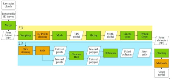
Figure 1.
Flowchart of CLOUD2FEM procedure [47].
A pixelated fusion method regarding solid model generation via actual points-based voxelization to carry out FEA is proposed by [49]. The flowchart can be found in Figure 2a. The input of this research is the point cloud which is segmented from light detection and ranging (LiDAR) data. The asterisk in Figure 2a means the preparation of LiDAR and detection of the building object involve multiple steps outside the scope of this reference’s scientific contribution. Most previous voxelization methods focus on the surface representations of structures. Hence, the key step of these methods must identify through which voxels the surfaces pass [49]. By contrast, as it is shown in Figure 2b, the innovation is in the voxel generation step. The voxelization based on point clouds in this research operates on the points data directly. Taking the measured points as internal points, the hexahedral elements are created around them. In this process, the surface derived is not required. The pixelated model is obtained. The resulting pixelated model maps directly to the FE discretization model to realize the whole FE computation process.
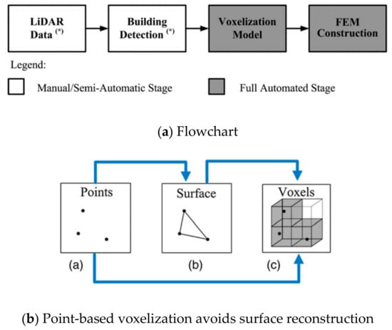
Figure 2.
(a,b) Pixelated method about solid model generation [49].
A new fusion model strategy for the FE computation is presented in [48] which integrates TLS, deviation analysis, and FE computation. The reference objects with respect to the plane, sphere, cylinder, and cone are optimized through the deviation analysis. The computation of the distance between the point clouds and reference shapes are obtained to provide local deviations. Hence, well-described geometric deformations can be obtained by this comparison in the deviation maps. A 3D FE model is constructed in this way with high accuracy.
In [50] the authors introduce an automatic method which is similar to the method in [47,48] but performs better. The mesh model transformed from point clouds is constructed by four-node tetrahedral elements. Nodes from the bottom part are projected to the horizontal plane for the easy operation of the boundary conditions. The re-topology step is carried out to obtain optimized solid meshes. The mesh model is characterized by a large reduced number of solid finite elements.
An updated numerical mesh model is proposed to obtain the knowledge of the actual structural behavior in the current damaged objects [51]. Damaged structure features are described in the mesh model. This is helpful to gather further in-depth insights into current conditions. Crack behaviors are identified in the final results [51]. This plays a critical role to guarantee the good accuracy of the FE computation.
There are two different disciplines in the development, CAD and CAE, while different model representations are requirements [52]. Consequently, the integration of both CAD and CAE is a key step. Most methods introduced in this section focus on meshing the CAD geometry and combining the meshes with a CAE discretization model. Other branches, B-spline and NURBS approximation introduced in Section 1.2, representing the CAD model, are developing rapidly. Many researchers have made great contributions in this topic.
The IGA is a significant product used for solving problems regarding structural mechanics, solid mechanics, and the fluid field [25]. The NURBS-based IGA method outlined in [24] integrates the accurate geometric design with analysis. This is discussed mainly in Section 1.2. However, major shortcomings are obvious in this method. The greatest difficulty is that IGA makes mesh generation complicated in the computation [25]. This is still a highlighted topic to be developed in the FE computation.
In recent years, a methodology framework has been suggested to integrate the highly accurate two-dimensional (2D) model into the commercial simulation software ANSYS, which shows possibilities to provide a suitable and accurate CAD model for FE computations [6]. This framework also offers a brief to construct a 2D FE geometry with TLS. The integrated geometry is based on B-splines. After the extraction of the point clouds measured by TLS, B-spline is applied to approximate the external structure of the arch concerned, as is shown in Figure 3. Obtained B-spline points are converged to describe the 2D geometry. The B-spline-based geometry captures the deformed details and gaps accurately. The error rate regarding the average displacement is obviously improved when the computational model applies the B-spline-based 2D model.
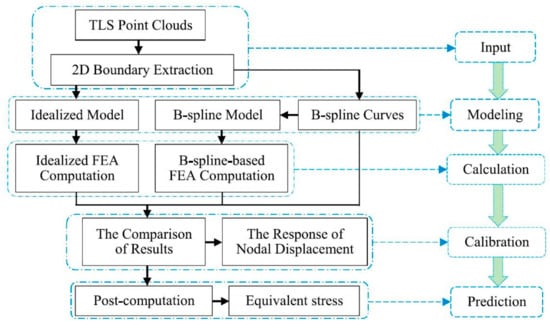
Figure 3.
The framework of B-spline-based computation [6].
1.5. Motivation and Framework
The common mechanical and structural models contain unknowable deformations after the unexpected mechanical process. It is necessary to apply advanced measurement methods to detect the accurate deformed surface information. This research focuses on the FEA based on the parametric model by approximating point clouds from TLS. It is expected to apply the parametric approximation method to improve the accuracy in describing the measured data of 3D structural surfaces. Therefore, the entire FE model of composite structures can be generated in a novel parametric method. The parametric model provides a continuous and parametric expression that can be applied in both CAD and CAE. This method makes up for the shortcomings of the FE geometric description regarding the discontinuity of the mesh-based model in Section 1.4. The final goal is to reduce computation errors in FEA due to the geometric simplification of structural models.
A reliable FE computation can decrease the number of actual experiments and reasonably reduce the expensive cost of the experiments. Therefore, improving the computation accuracy has become one of the key goals in the FE computation process of structural problems [53,54,55,56].
The general method to carry out the structural analysis is to apply the simplified model mainly. This method is separated into three steps, as is shown in the blue parts of Figure 4. The first step is to idealize the detailed structures into simplified CAD geometries or designed geometries. The main features following the geometric details in the simplification process are normally the height, the width, the length, and the thickness. The second step is to transfer the CAD model to the CAE model. The third is to compute the CAE model. This is a scientific and significant method if the task is to design and improve the object structure in the computations of structural problems [57,58]. However, there is an inaccurate simplification when the structure contains detailed gaps and irregular parts. It is essential to describe the detailed structures in a more scientific and accurate way.
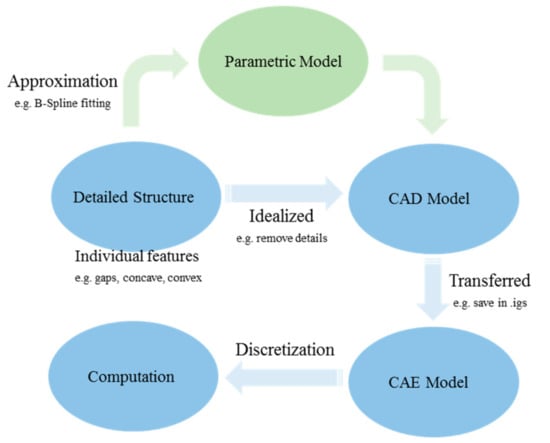
Figure 4.
Model computation progress.
Accurate model approximation of the structural problem leads to more physically accurate results in the final computation process. The mesh discretization of the geometry based on point clouds is a significant method to obtain accurate model reconstruction, which was confirmed in the previous Section 1.4. Their main advantage lies in their continuity characteristic describing surfaces and curves. Attempts to apply B-spline curves in a 2D arch model indicates and validates the significance of the parametric model for the FEA [6]. However, it should be noticed that the main limits lie in the discontinuity of the discretized model description. This can lead to incompatibilities in processing grids using different commercial FE computation software. Therefore, if an effective geometric description that satisfies the continuity requirements is provided, the discontinuity problem of the mesh discretization can be avoided. Using the IGA concept developed, it is found that B-Spline or NURBS-based geometry description can improve the smoothness and accuracy of the parametric model. There is no mature and significant technology on the practice of B-spline-based or NURBS-based numerical model description for very complex objects [59]. Therefore, this still needs to be developed, especially in the case of dealing with complex parametric structures characterized by more irregularities and deformations.
Since the accurate free-form property of B-splines is so beneficial, this research chooses this method to generate the parametric model for the FEA. As it is shown in the green parts of Figure 4, the parametric model is created here as a mediation tool. The approximation task of point clouds measured from TLS can be accomplished by B-spline fitting. In this case, the advanced parametric model can meet the continuity requirement and, subsequently, be adopted in commercial FE computation.
Attention should be paid to the fact that the choices of measurement methods are diversified. Many excellent and efficient methods have been developed, e.g., TLS, digital photogrammetry, and radar technology [60]. The data measured to generate the parametric FE model in this research is acquired by means of TLS. In other references, the radar, the photogrammetry, and the integration technologies of multi-sensors can also be alternatively developed to measure the geometry surface information [38,39,40,41,42,43]. Analogously, the T-spline method, and NURBS approximation can be an alternative to the B-spline methods in fitting the geometric surface.
There are five main sections in this paper. Section 1 describes the geometric generation and advanced measurement methods regarding structural problems. A contrast analysis is carried out to understand the advantages and disadvantages of different methods comprehensively. Meanwhile, the kernel motivation and the overall framework of this paper are declared. Section 2 discusses the key methodology of the parametric model and applies the novel parametric model in the FEA. The process to acquire the data measured, the parametric function of B-spline approximation, and the model generation steps are listed in detail in this section. Section 3 applies the parametric model regarding structural problems into a FE computation and computes the results in both the static structural and dynamic computations. Section 4 discusses the static and dynamic computation results and analyzes the model quality based on point clouds, the errors between the parametric model and the simplified model, and the result deviations between both models regarding the static and dynamic computation. Section 5 draws the main conclusions of this paper.
2. Methodology of the Parametric Model
The methodology of the parametric computation regarding the structural problems contains four main steps in total: the measurement, the parametric approximation, the parametric modelling, and the computation, as is shown in Figure 5. The common computation method constructs the target object as a simplified form in the CAD modelling software, which only keeps basic features regarding some sizes, while the deformed details are omitted. Measurement experiments with accurate sensors are desired, which aims to reconstruct the deformed information. Measured data is converted to the available parameter set and then extracted into different features. The 3D model can be fitted by the B-spline volume directly if the model shape is not complex [28], which is not common in structural problems. Therefore, volume features are further decomposed into surface patches. The B-spline surface approximation is applied to fit the decomposed surfaces. The final parametric surfaces are only acceptable when the fitting accuracy is satisfactory. The parametric surfaces are converted to the CAD modelling software. The parametric geometric modelling is processed based on the parametric surfaces and transformed into the computational model. Lastly, the computation progress can be accomplished after the mesh generation and boundary condition application. Kernel links are listed in the next sections in details and applied into a composite structural building.
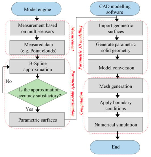
Figure 5.
The flow chart of parametric methodology.
2.1. Feature Acquisition of the Object
In the feature acquisition progress, it is initially necessary to obtain the global feature of the target object through measurement methods by advance sensors. A TLS-based sensor system is adopted in this step. Secondly, the task is to transform the large datasets into the key and useful coordinate values. Thirdly, the patch decomposition is carried out due to the discontinuity characteristics in the right angle parts, which is ubiquitous for complex building and mechanical structures. There are also some windows, entrance and exit passages, and non-removable parts on the surfaces. Finally, as a result, it is necessary to recognize the boundary features that represent windows, passages, and non-removable parts. In the following, the detailed experiment and operations are introduced to obtain the object feature with the application of these steps.
The researched object is used on the basis of a composite structure regarding a warehouse building with a north-wall length of about 16 m, south-wall length of about 16.5 m, width of about 14.2 m, height of 3.6 m, and wall thickness of 0.2 m. The point cloud of this structure is sample data from PointCab GmbH which offers powerful software to make the processing of high-resolution point clouds easy. It also offers open access for users to download sample data regarding point clouds. The aim is to research weak situations and positions in this deformed structure by combining TLS with the FE computation. The TLS equipment (FARO FocusS 350) and laser tracker equipment (FARO Laser Tracker Xi) were used here to obtain the 3D point clouds [46,61,62,63]. The systematic distance error of this type TLS is. The vertical and horizontal resolution of the TLS is. The maximum vertical scanning speed of the TLS is. The laser tracker, which has an angular accuracy of in angle measurement performance, is applied for the purpose of reference and validation.
The scanning positions are separated into three parts, as it is shown in Figure 6 from the top view. The north direction is marked as N here. There is a total of 13 positions for scanning totally. From the ground-based scanning positions outside the building, there are five positions to capture the outside details: 1, 2, 3, 4, and 5. There are also five scanning positions inside the building: 6, 7, 8, 9, and 10. There are normally only one or two scanning positions inside such a building. However, there are four forced pillars inside the building. Consequently, the number of scanning positions is increased to five to capture the details of the forced pillar. The final scanning positions 11, 12, and 13 are based on the building roof.
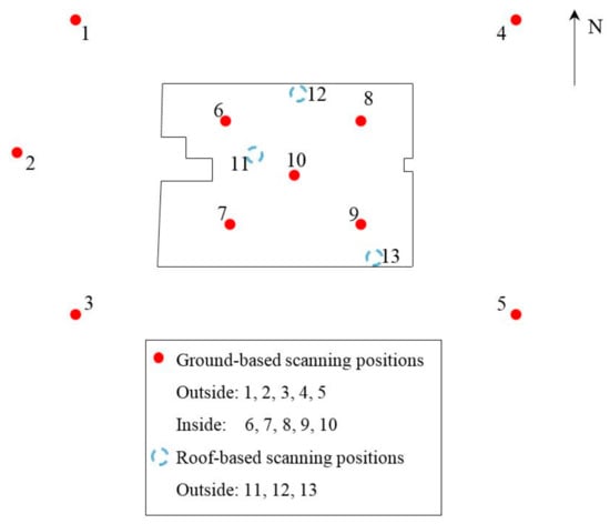
Figure 6.
Terrestrial laser scanning (TLS) scanning positions.
The point clouds measured from PointCab contain not only the data needed, but also the unexpected noisy points. A smoothing operation is commonly applied when the initial images are dealt with. This is known as blurring. The role of the smoothing operation here is to reduce the noisy points in point clouds from the TLS. The Gaussian Filter applying the OpenCV function “GaussianBlur” is adopted in this research. The size value and application of the function can be referred to in [64]. The detailed structure of this warehouse building can be found in the point clouds of Figure 7 after the smoothing operation. There are coordinate, scalar, RGB color, and normal values in the scanning results. The kernel information in Figure 7 is the coordinate value of every point which is finally extracted as a P matrix by deleting the unexpected values in MATLAB R2018b, see Equation (1).
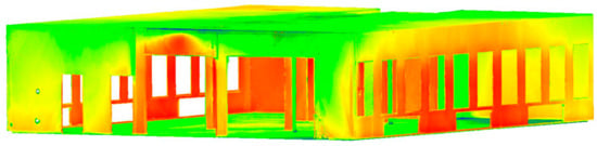
Figure 7.
Reflectance image from TLS point cloud.
The focus of this research lies in the reconstruction of the complex composite structures with unknown deformations based on the parametric solution. Hence, points on the volume are firstly decomposed into points on the surface patches. The parametric solid volume is assembled again by these patches after accomplishing the appropriate surface approximations. This is the solution to reconstruct the parametric solid model in this research. The decomposed patches are shown in Figure 8.
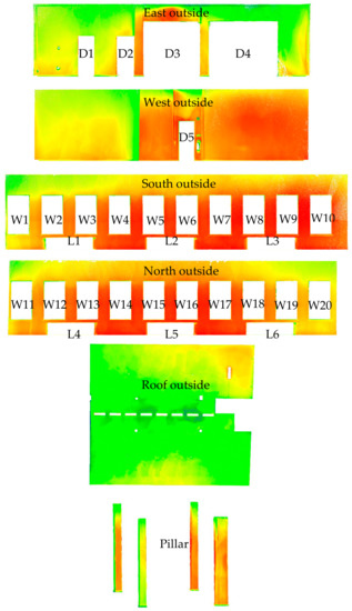
Figure 8.
Decomposition diagram of point clouds.
As shown in Figure 8, the global volume is decomposed into five parts which are marked as east, west, south, north, and pillar. The door, window, and lower window features are represented as D1 to D5, W1 to W20, and L1 to L6, respectively. The following fitting process is based on the continuous B-spline surfaces. Consequently, surfaces connected with right-angle interface layer should be subdivided into smaller patches. The east outside wall in Figure 9, which is implemented in the open access software CloudCompare V2.8, is subdivided into five patches by blue dotted layers. The purpose is to guarantee the continuity of every independent patch. As a result, the subdivision is adopted in other parts in Figure 8, which is followed by the same method in Figure 9. The boundary extractions of the window and door features apply the boundary threshold method [6] using the principle of Delaunay triangulation [64,65] with a threshold value of 10 mm. The aim of this extraction is to recognize the boundary features of different surfaces for the future trimming step in the B-spline surface.
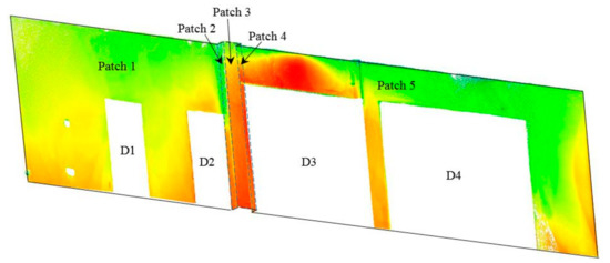
Figure 9.
Subdivided patches of east outside wall.
2.2. B-Spline Approximation
2.2.1. B-Spline Basis Function
Given a knot vector, the B-spline basis function starts with a zeroth order basis function () as is shown in Equation (2). It is known as the Cox–deBoor recursion function [66]. The values of are elements of knot vectors. Here, the parameter is the coordinate in the parametric space that is needed to satisfy the relationship in Equation (2). The parameter varies from the minimum value to the maximum value along the calculated curve.
The B-spline basis functions are defined recursively by Equation (3), for. is the degree of the basic function. Here, it is possible for the status during the molecular formula computation in Equation (3) to behave in special situation asin the ratio of the numerator and the denominator. The convention of this special situation is to default this as 0 in the recursion work. For detailed explanations, please refer to [12,67].
2.2.2. B-Spline Curves and Surfaces
The last remaining step is to create the control points of the B-spline. They form the so-called control polygon in the calculation. Interested readers can refer to [12,13,63] for more details regarding the B-spline parameter calculation.
The B-spline curve can be constructed by linearizing the B-spline basis functions, as is given by Equation (4). Coefficients of the basis functions are referred to as control points.
The B-spline surface is represented as Equation (5), which is a tensor product of B-spline curves. The control points of the B-spline surface form a control net,, and are basis functions of B-spline curves which approximate B-spline curves in two directions.
2.2.3. B-Spline Approximation
The first B-spline approximation task is based on curves which are of significance to describe different feature boundaries of the structure, for example, windows and doors. The degree value of basis functions is 3 [6,67]. The values of the control point number of different feature boundaries regarding the east side wall in Figure 9 are listed in Table 1. Four feature regions have to be extracted on the east outside surface. Ground-based sides of each feature are ignored. Other sides obtain reasonable numbers of controlled points as is shown in Table 1, which are referred to in detail in [12,63]. The extracted B-spline feature curves are then applied as the trimming and projection boundaries to the B-spline surfaces.

Table 1.
Numbers of control points of B-spline curves regarding feature parts.
Aiming at reconstructing the solid parametric model of composite structures, the surface-based approximation is a key step in the reconstruction step. Taking the south side surface as an example, the deformed surface is approximated as a parametric surface with the application of B-splines, as is shown in Figure 10a. The degree value of the basis functions is 3. The degree value can be adjusted according to the approximation demands. The choice in this manuscript is based on previous papers [6,63]. The control points are distributed in two directions in the surface fitting process, as mentioned in Equation (5). In the south surface example, numbers of control points are 36 in the height direction and 165 in the length direction. The accuracy characteristic of B-spline surfaces in [6,63,67] is proved which adopts 20 control points in the approximation progress regarding an arch structure with the length of 2 m, which indicated that there is a control point every 0.1 m. The determination regarding the quantity of control points affects the quality of the approximated surface. Detailed explanations regarding the parameter and model selection problem are given in [63]. The length of this surface is about 16.5 m. The height is about 3.6 m. Hence, control points are added to the model every 0.1 m in this example. The standard deviations are calculated in Section 4.1, which indicates that the quality of the parametric model is more accurate than the simplified model. Consequently, the number of the control points can be considered as reasonable and reliable in this computation.
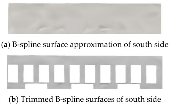
Figure 10.
(a,b) B-spline surface approximation of the south side surface.
Parametric surface trimming is a complex activity [68]. The shape of B-spline curves regarding the feature parts are not absolutely compatible with the shape of the B-spline surface due to the uncertainty of the boundary extraction progress. Hence, the surface trimming step is of great significance to obtain accurate boundary recognition regarding the feature parts in the solid model. The final B-spline surface with window features after trimming is shown in Figure 10b.
3. Finite Element Method
3.1. Computations
The final reconstructed parametric model and the designed simplified model are shown in Figure 11. The simplified model here is a similar model that keeps the same length, width, height, and thickness as the measured data. It also ensures the same small feature parts, for example, windows, doors, and holes. The most obvious difference is that the parametric model contains the detailed deformed surfaces while the simplified model is constructed with flat surfaces only. Deformed surfaces regarding this building are obtained by the TLS. The description of these deformed surfaces takes advantage of the B-spline approximation to fit the point clouds. The surface features can be found in the dark parts of Figure 10a,b. The detailed analysis regarding the model quality and accuracy is discussed in Section 4.
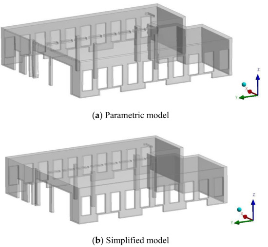
Figure 11.
(a,b) Reconstruction of parametric and simplified models.
It should be noticed that the final reconstructed model only generates the detailed geometric surfaces from the TLS data. The internal information regarding the material should be taken into account in the future.
Here, the pillar parts consist of reinforced concrete, as is shown in Figure 12. Hence, the reinforced concrete characteristic [69] is added into the final composite structures based on the parametric and simplified models. The diameter of the reinforcement is 25 mm. One pillar contains four steel bars. The concrete density applied here is. The Young’s modulus and Poisson’s ratio of the concrete are and , respectively. Additionally, the reinforcement is structural steel material, which contains the density of , Young’s modulus of , and Poisson’s ratio of . The reference temperature of the reinforcement is the same as that of the concrete. The properties of the concrete and the reinforcement are listed in detail in Table 2. The reconstructed composite models after compounding the characteristics of the reinforcement and the concrete are finally computed in the ANSYS Workbench software.
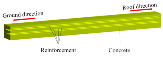
Figure 12.
Reinforced concrete pillar.
Table 2.
The main properties of the computation.
There are many future behaviors and loading types of the structural problems. The structural loading and small vibrations are common destructive performances in engineering [48,70]. Hence, the force-loading and vibration progresses are two main reasons leading to the possible future behaviors. This manuscript compute two kinds of mechanical behaviors based on the static and dynamic analysis.
In the static analysis based on the force-loading computation, surfaces in contact with the ground are defined as fixed supports. The roof surface is loaded with a 2 kN force in the negative direction of coordinate z. The overall loading process is based on the static structure computation. The aim of this computation is to find the weak zones in different models and validate the significance of the parametric model in a static structure analysis.
The dynamic analysis in this computation focuses mainly on the vibration computation based on the modal computation. It is combined with the random vibration module. The aim is to evaluate the response characteristics of different model structures in dynamic processes. Here, surfaces in contact with the ground are set as fixed supports in the dynamic computation.
3.2. Static Computation Results
The deformation results regarding both models in the static structure computation are shown in Figure 13. The red color bar in this figure indicates the largest deformation zones in the deformation progress. The maximum deformation of the parametric model is 0.193 mm, which appears in the north-central location. The maximum deformation 1.36 mm of the simplified model appears in the central part, which is seven times the value of that in the parametric model. One of the possible reason is the wall weight difference between the two models. From the perspective of Figure 13, small deformations can be found in the north side wall of the parametric model. It should be noticed that both models contain the similar deformation diffusion and development laws generally.
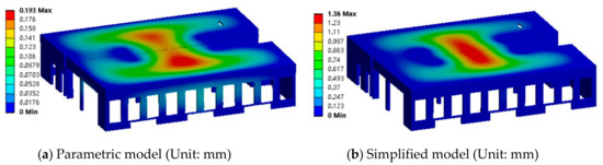
Figure 13.
(a,b) Deformation of parametric and simplified models.
3.3. Dynamic Computation Results
In the dynamic computation, the focus of this paper is based on the modal analysis regarding the structure which is a basis of the vibration analysis. It indicates natural frequencies and mode shapes of this structure. Figure 14 shows the deformation shape in different modes of two models.
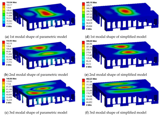
Figure 14.
(a–f) Different modal shapes of parametric and simplified models (unit: ×10−3 mm).
Generally, the deformation contour based on the vibration computation is different with those based on the static computation. The modal shapes in different modal conditions regarding the same model are completely inconsistent. The maximum modal deformations in the parametric model are 159.94 × 10⁻³ mm, 159.95 × 10⁻³ mm, and 146.06 × 10⁻³ mm, while the maximum modal deformations in the simplified model are 445.18 × 10⁻³ mm, 388.08 × 10⁻³ mm, and 402.23 × 10⁻³ mm, respectively. The development laws regarding the maximum modal deformation are inconsistent. This indicates that the dynamic results in the simplified model computation are invalid. Hence, the accurate parametric model is necessary in the composite structural computation and it is beneficial to improve the reliability and accuracy of the behavior prediction in the FEA progress.
4. Discussion and Analysis
This research is based on the model reconstruction of the composite structures. The evaluation of different models is unknown. Consequently, it is necessary to validate the model quality and describe the main effects due to the model deviations in following subsections. Section 4.1 discusses the quality of the reconstructed model itself and the deviation between the measured point cloud data and reconstructed models. Section 4.2 analyzes the deviations between two researched models. Section 4.3 extracts the deformation contour of both models into one figure and analyzes development laws regarding the deformation. Section 4.4 carries out a detailed discussion regarding the stress result. Section 4.5 analyzes the modal features of the dynamic computation.
4.1. Model Quality Based on Measured Data
Model errors based on different surfaces are listed in detail in Table 3 in order to determine the model qualities. The error analysis is based on the comparison between the point cloud matrix P and the analyzed model surfaces. The standard deviation is calculated by Equation (6). In the parametric model based on B-splines, the standard deviations of all fitting surfaces are about or within 1 mm. The maximum standard deviation is 1.15 mm which is on the south outside surface. The maximum standard deviation in the simplified model is 22.56 mm which is on the north outside surface.
Table 3.
Approximation deviations of surfaces.
The maximum deviations in the parametric model are in the interval of [26,51] mm. These values are much larger than the standard deviations. This is due to the remaining noise points on these surfaces. Hence, the maximum deviation also partly contains outliers. The standard deviations of the east, south, and north surfaces are larger than that of other surfaces from Table 3. It is also obvious from Figure 8 that the boundary regions of door or window features are large. The possible reason for the larger standard deviation is that some outliers exist in large boundary regions in the TLS measurement. Both maximum and standard deviations in the simplified model are obvious due to neglecting of the surface deformation in the reconstruction progress of the simplified model.
Generally speaking, the approximation quality of the parametric model behaves superior to that of the simplified model on the basis of surface deviation comparisons, which is indicated in Table 3. The average approximation accuracy of the parametric model can reach the millimeter level. The maximum deviations of all outside surfaces in the simplified model are dozens of times larger than the corresponding standard deviations in the parametric model. This indicates that the simplified model is far from the true measured data.
The standard deviation of the parametric model can still be reduced by increasing the control points and adjusting the order of basis functions in the approximation progress of the composite structures. However, the calculation cost and the workload of the model reconstruction will increase greatly. Meanwhile, the mesh generation and the FE computation will be more complex. As a result, the global computation of the parametric model will perform extremely inefficiently in this condition. In this manuscript, the object researched is a large scale model. It is important to balance the calculation cost and computation accuracy. The present accuracy of the parametric model is much higher than the accuracy of the common simplified model. The determination of the geometric accuracy differs in different scale simulations. The computational model reconstruction of details in composite structures with multi-scales can be improved by adjusting control points and basis function orders based on multi-scales.
4.2. Deviation Analysis of Two Models
Details about the centroid position and moment of inertia regarding to different models are extracted in Table 4. The mass volume refers to the size of the volume filled with model materials, which differs from the common solid enclosed volume. The mass volume of the simplified model is 67.8 m3, which is 88.6% of the mass volume of the parametric model. This indicates the weights of both models are different. As is generally known, the deformation exists when the force is loaded on the non-ideal rigid body. Therefore, the effects due to the different self-weights cause different predeformation effects. Hence, the computation based on the simplified model brings predeviation before the FE computation.
Table 4.
Properties of solid models.
The centroid positions are listed in Table 4. The local origin points of both models are set at the endpoint on the north lower side of the east outside surface. The local origin point coordinate in the global coordinate system of the simplified model is (0, 10.1, −9.9) m. The local origin point coordinate in the global coordinate system of the parametric model is (−21.2, −6.8, 0.2) m. The relative centroids in the global coordinate system can be calculated by Equation (7). In this equation, is the coordinate of the relative centroid, is the coordinate of the centroid in global system, and is the global coordinate of the local origin point of each model. The coordinates of each relative centroid are shown in Table 4, respectively. The coordinate difference between two relative centroids is (0.4, 0.5, 0.26) m, respectively. The deviation rate of the centroid coordinate based on the parametric model centroid is about (5.3%, 5.8%, 9.4%). As a result, the deviation rate of the moment of inertia in different directions is (4.8%, 6.7%, 6.1%). While the moment of inertia is greater, the ability to resist deformation of the object is stronger. Hence, the difference of the centroids and moments of inertia is also a possible reason for the deformation deviation after loading.
Surfaces in the simplified model are all based on flat planes. The surface of the simplified model constructed in this research is described by Equation (8) which is a plane. Hence, the distance of the B-spline surface point in the parametric model to the simplified flat surface is obtained by Equation (9). . The total amount of approximated B-spline points is. The global average deviation between the B-spline surface and the simplified surface can be indicated by Equation (10). Hence, the global average deviation regarding 11 surfaces can be calculated by Equation (11). The final average deviation of the global surfaces is 8.76 mm. This value indicates the obvious shortcomings of the simplified model which is applied commonly. The parametric model describes the deformed details on all surfaces with the advantage of B-splines. However, the simplified model reconstructs the surfaces as idealized and flat ones and ignores the deformation information description. This is the main reason for this obvious deviation between both models.
In summary, it is of great significance to compare the deviation performance when the geometric models of structural problems are reconstructed before the FE computation. The deviations between the parametric and the simplified models are obvious. The mass volume of the parametric model is larger than that of the simplified model which results in the deviation of the predeformation due to the self-weight. The relative centroid of the parametric model offsets from the simplified model relative centroid in the global coordinate system. The average deviation between two models is finally very large, which leads to influence the parametric model in the model selection progress regarding the structural problems.
4.3. Deformation Analysis Based on Static Structure
Aiming at researching the effect of different geometries on the FE computation, it is of significance to carry out the deformation analysis. The deformation contour figure regarding different deformation values of the roof surface is extracted in Figure 15. The blue lines indicate deformation results based on the parametric model, while the red dashed lines show the deformation results based on the simplified model. The centroids of both models are marked in this figure.
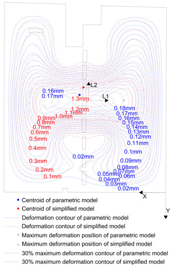
Figure 15.
Deformation contour of parametric and simplified models.
The deformation contour spacing of the parametric model in the L1 positive direction gradually decreases from the maximum deformation zone, while that in the L2 positive direction decreases initially and then increases. There is the same changing law of the deformation contour in the simplified model. Here, 30% of the maximum deformation is defined as the large deformation zone, which is marked as a red solid line in the simplified model and a blue dashed line in the parametric model. It is obvious that the total areas regarding both large deformations are similar. With the decrease of the deformation, the contours of both models are closer. This indicates that the simplified model can also fit a relatively accurate deformation-changing law outside the large deformation zones.
Obvious differences between both models are the maximum deformation positions and large deformation zones. The maximum deformation position in the simplified model is almost in the center of the roof surface. With the application of the parametric model, this position moves to the positive direction of L1 and L2. However, the deviation of two maximum deformation positions in the L2 direction is not as obvious as that in the L1 direction. With the combination of the centroids in Figure 13, the relative position of two centroids is opposite to the relative position of the maximum deformation points. The reason focuses on the effect of the centroids’ position and values of moments of inertia in different directions. With the movement of the centroid to the left and lower sides, here from the simplified model to the parametric model, the anti-deformation ability in the left and lower zones improves in the parametric model. Consequently, the large deformation zone of the parametric model moves to the right and upper direction when compared to the simplified model. The large deformation position changes more obviously in the L1 direction than in the L2 direction. This is due to the geometric characteristics of this object. From the relative perspective in Figure 13, the left and right sides are, respectively, the south and north surfaces of the building. Their architecture and locations are more symmetrical. However, due to the existence of the obvious concave part in the upper zone, this feature structure can better support the loading force of the object. Therefore, the large deformation zone does not move upwards obviously.
4.4. Stress Analysis Based on Static Process
Equivalent stress is of great significance to monitor the strength of the damage possibility in the loading progress, as it is shown in Figure 16.
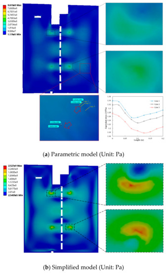
Figure 16.
(a,b) Equivalent stress of parametric and simplified models.
The color difference in the deformed zones of the surfaces is obvious. This indicates the stress change. There are two concave strip shapes in the red enlarged area of Figure 16, while the equivalent stress contour of this zone is smooth in the simplified model of Figure 16b. The equivalent stress of the upper concave peak part is 125.24 MPa, while the equivalent stress of the concave valley part is 123.93 MPa. The equivalent stress of the lower concave peak part is 131.99 MPa, while the equivalent stress of the concave valley part is 130.49 MPa. Three line examples are extracted in the same concave change part. The length is about 0.2m which is close to the width of the concave region. The equivalent stress along the line length is listed in this figure. It indicates that the deformed concave shape affects the stress results. By contrast, this detailed feature cannot be found on the flat surface of the simplified model. It indicates that the deformed surfaces have a direct effect on the surface stress behaviors in the loading progress. There is a great difference regarding the maximum equivalent stress between the parametric model and simplified model, which is enlarged as the black dashed frame zones in Figure 16. Two black enlarged zones in the simplified model show that the maximum equivalent stress on the roof surface is close to the maximum value of the global model. However, the maximum stress of the parametric roof surface is far less than the global maximum stress value. The damage behavior in the engineering application will be predicted inaccurately if the parametric model is ignored.
The contour shape regarding the large stress zone of both models is generally similar. There is a similar development law of the equivalent stress contour if the specific value is not considered seriously. Consequently, similar models contain similar stress development laws in the same conditions. Hence, the common simplified model can be reasonably adopted in the computation of structural problems when the research focus is on the overall laws because the simplified model is more efficient.
4.5. Vibration Analysis
Modal analysis is the basis of the dynamic structural computation. With the help of the modal analysis, it is helpful to recognize different responses of the structural problems to different dynamic loadings. The vibration analysis involves a wide range of knowledge. However, this research focuses on the analysis of two reconstructed geometric models. Therefore, only a contrast dynamic analysis between two models is carried out based on the frequency and the vibration deformation.
The relative modal data in Table 5 are beneficial for comparing the vibration characteristics of the structural problems [71]. Error 1 calculates the relative deviation regarding the maximum vibration deformation between the parametric and simplified models. Error 2 calculates the relative deviation regarding the modal frequency of two models. Two errors are obvious, which implies the inadequacies of the common simplified model. By contrast, the maximum deformations of the parametric model in the 1st, 2nd, and 3rd modal conditions are far less than those of the simplified model, while the frequencies in the parametric model are higher than in the simplified model. This indicates that the parametric model is more capable in the dynamic computation of structural problems.
Table 5.
Contrast vibration analysis between two models.
5. Conclusions
This manuscript offers a generic methodology which focuses on the FEA based on the parametric model by approximating 3D actual feature data. 3D actual feature data can be acquired from many efficient measurement methods, e.g., TLS, digital photogrammetry, and radar technology. The methods in approximating parametric surface models accurately are diverse, e.g., the T-spline method, the B-spline method, and NURBS approximation.
It was applied to detect the deformed surface information by TLS which is an accurate and reliable measurement technology in this research. The B-spline method was applied to approximate the measured point clouds data and generate the parametric 3D model of structural problems. The parametric model can be applied in both CAD modelling and CAE analysis innovatively. The model quality and some deviations were discussed. The static and dynamic computations were carried out to imply the advantages and disadvantages of both models regarding the responses of different loadings. The main conclusions are as follows.
1. The numerical parametric model of structural problems satisfies the continuity characteristic in constructing the 3D model with the advantage of the parametric description method B-splines.
2. The parametric model can reserve deformed features of the structures accurately. When the data measured is compared, both the maximum and standard deviations of the parametric model are far less than the simplified model. The mass volume of the simplified model is smaller than that of the parametric model due to the lack of the description of deformed walls. This is one of the main reasons why there are obvious deformations between the parametric and simplified models in the static and dynamic computations.
3. In the static structural analysis, the simplified model is acceptable and it is more convenient and efficient to analyze and predict the overall development law regarding the deformation and stress outside the large deformation zones. The simplified model has obvious shortcomings and inaccuracies in large deformation zones compared to the parametric model in the static structural computation.
4. The FEA computation based on the parametric model is more reliable which benefits from the parametric description of the actual object, e.g., B-Spline method.
5. The parametric model contains fewer errors in the dynamic computation. It indicates that the parametric model is more reasonable and acceptable in the dynamic computation and analysis, especially in the large deformation and stress zones.
6. There is an obvious effect of predeformed parametric surfaces on the equivalent stress of the composite structures in the loading progress. Therefore, the parametric model is more accurate in predicting the future behavior by analyzing the equivalent stress of composite structures.
Attention should be paid to the fact that the FEA model simplification can bring some efficiency to researchers to a certain extent, e.g., when the research purpose is only to predict some simple regularity problems or development trends. However, numerical features, e.g., the deformation, the stress, and the strain, should be focused on significantly in most cases when it is in the accurate design, optimization, and prediction stages. Therefore, the FEA model simplification is not desirable in this case and the accurate parametric model is significantly desired.
In summary, the FEA based on the parametric model is instructive for understanding the structural progress and predicting the damage behaviors in this paper. The novel parametric model method is efficient and beneficial to improve the reliability and accuracy of the FE computation regarding the composite structural problems. Moreover, it is of great significance to apply the FEA parametric model to health to monitor the future damage behavior of the composite structures in the engineering application.
Author Contributions
W.X. wrote main parts of the paper, analyzed the data and performed the 3D computation. I.N. supported with consultations and carried out the final review and proofreading of the paper. All authors have read and agreed to the published version of the manuscript.
Funding
The publication of this article was funded by the Open Access fund of Leibniz Universität Hannover.
Acknowledgments
Authors gratefully acknowledge the use of the sample data of PointCab GmbH for this research.
Conflicts of Interest
The authors declare no potential conflicts of interest with respect to the research, authorship, and/or publication of this article.
References
- Stefanou, G. The stochastic finite element method: Past, present and future. Comput. Methods Appl. Mech. Eng. 2009, 198, 1031–1051. [Google Scholar] [CrossRef]
- Hou, T.Y.; Wu, X.H. A multiscale finite element method for elliptic problems in composite materials and porous media. J. Comput. Phys. 1997, 134, 169–189. [Google Scholar] [CrossRef]
- Holzapfel, G.A.; Gasser, T.C.; Ogden, R.W. A new constitutive framework for arterial wall mechanics and a comparative study of material models. J. Elast. 2000, 61, 1–48. [Google Scholar] [CrossRef]
- Birman, V.; Byrd, L.W. Modeling and analysis of functionally graded materials and structures. Appl. Mech. Rev. 2007, 60, 195–216. [Google Scholar] [CrossRef]
- Pramod, A.L.N.; Ooi, E.T.; Song, C.; Natarajan, S. Numerical estimation of stress intensity factors in cracked functionally graded piezoelectric materials—A scaled boundary finite element approach. Compos. Struct. 2018, 206, 301–312. [Google Scholar] [CrossRef]
- Xu, W.; Xu, X.; Yang, H.; Neumann, I. Optimized finite element analysis model based on terrestrial laser scanning data. Compos. Struct. 2019, 207, 62–71. [Google Scholar] [CrossRef]
- Gómez, S.; Vlad, M.D.; López, J.; Fernández, E. Design and properties of 3D scaffolds for bone tissue engineering. Acta Biomater. 2016, 42, 341–350. [Google Scholar] [CrossRef]
- Peng, X.; Atroshchenko, E.; Kerfriden, P.; Bordas, S.P.A. Isogeometric boundary element methods for three dimensional static fracture and fatigue crack growth. Comput. Methods Appl. Mech. Eng. 2017, 316, 151–185. [Google Scholar] [CrossRef]
- Wang, D.; Hu, F.; Ma, Z.; Wu, Z.; Zhang, W. A CAD/CAE integrated framework for structural design optimization using sequential approximation optimization. Adv. Eng. Softw. 2014, 76, 56–68. [Google Scholar] [CrossRef]
- Breitenberger, M.; Apostolatos, A.; Philipp, B.; Wüchner, R.; Bletzinger, K.U. Analysis in computer aided design: Nonlinear isogeometric B-Rep analysis of shell structures. Comput. Methods Appl. Mech. Eng. 2015, 284, 401–457. [Google Scholar] [CrossRef]
- Montagnat, J.; Delingette, H.; Ayache, N. A review of deformable surfaces: Topology, geometry and deformation. Image Vis. Comput. 2001, 19, 1023–1040. [Google Scholar] [CrossRef]
- Piegl, L.; Tiller, W. The NURBS book, 2nd edition; Springer-Verleg: Berlin/Heidelberg, Germany, 1997. [Google Scholar]
- Bureick, J.; Alkhatib, H.; Neumann, I. Robust Spatial Approximation of laser scanner point clouds by means of free-form curve approaches in deformation analysis. J. Appl. Geod. 2016, 10, 27–35. [Google Scholar] [CrossRef]
- Park, H.; Lee, J.H. B-spline curve fitting based on adaptive curve refinement using dominant points. CAD Comput. Aided Des. 2007, 39, 439–451. [Google Scholar] [CrossRef]
- Yoshihara, H.; Yoshii, T.; Shibutani, T.; Maekawa, T. Topologically robust B-spline surface reconstruction from point clouds using level set methods and iterative geometric fitting algorithms. Comput. Aided Geom. Des. 2012, 29, 422–434. [Google Scholar] [CrossRef]
- Yoo, D.J. Three-dimensional surface reconstruction of human bone using a B-spline based interpolation approach. CAD Comput. Aided Des. 2011, 43, 934–947. [Google Scholar] [CrossRef]
- Gálvez, A.; Iglesias, A.; Puig-Pey, J. Iterative two-step genetic-algorithm-based method for efficient polynomial B-spline surface reconstruction. Inf. Sci. 2012, 182, 56–76. [Google Scholar] [CrossRef]
- Louhichi, B.; Abenhaim, G.N.; Tahan, A.S. CAD/CAE integration: updating the CAD model after a FEM analysis. Int. J. Adv. Manuf. Technol. 2015, 76, 391–400. [Google Scholar] [CrossRef]
- He, Y.; Qin, H. Surface reconstruction with triangular b-splines. In Proceedings of the Geometric Modeling and Processing 2004, Beijing, China, 13–15 April 2004; pp. 279–287. [Google Scholar]
- Kiendl, J.; Bletzinger, K.U.; Linhard, J.; Wüchner, R. Isogeometric shell analysis with Kirchhoff-Love elements. Comput. Methods Appl. Mech. Eng. 2009, 198, 3902–3914. [Google Scholar] [CrossRef]
- Qian, X. Full analytical sensitivities in NURBS based isogeometric shape optimization. Comput. Methods Appl. Mech. Eng. 2010, 199, 2059–2071. [Google Scholar] [CrossRef]
- Zhang, Y.; Bazilevs, Y.; Goswami, S.; Bajaj, C.L.; Hughes, T.J.R. Patient-specific vascular NURBS modeling for isogeometric analysis of blood flow. Comput. Methods Appl. Mech. Eng. 2007, 196, 2943–2959. [Google Scholar] [CrossRef] [PubMed]
- Xia, Z.; Wang, Q.; Wang, Y.; Yu, C. A CAD/CAE incorporate software framework using a unified representation architecture. Adv. Eng. Softw. 2015, 87, 68–85. [Google Scholar] [CrossRef]
- Hughes, T.J.R.; Cottrell, J.A.; Bazilevs, Y. Isogeometric analysis: CAD, finite elements, NURBS, exact geometry and mesh refinement. Comput. Methods Appl. Mech. Eng. 2005, 194, 4135–4195. [Google Scholar] [CrossRef]
- Nguyen, V.P.; Anitescu, C.; Bordas, S.P.A.; Rabczuk, T. Isogeometric analysis: An overview and computer implementation aspects. Math. Comput. Simul. 2015, 117, 89–116. [Google Scholar] [CrossRef]
- Buffa, A.; Sangalli, G.; Vázquez, R. Isogeometric analysis in electromagnetics: B-splines approximation. Comput. Methods Appl. Mech. Eng. 2010, 199, 1143–1152. [Google Scholar] [CrossRef]
- Xu, G.; Mourrain, B.; Duvigneau, R.; Galligo, A. Analysis-suitable volume parameterization of multi-block computational domain in isogeometric applications. CAD Comput. Aided Des. 2013, 45, 395–404. [Google Scholar] [CrossRef]
- Bazilevs, Y.; Calo, V.M.; Hughes, T.J.R.; Zhang, Y. Isogeometric fluid-structure interaction: Theory, algorithms, and computations. Comput. Mech. 2008, 43, 3–37. [Google Scholar] [CrossRef]
- Bazilevs, Y.; Calo, V.M.; Cottrell, J.A.; Evans, J.A.; Hughes, T.J.R.; Lipton, S.; Scott, M.A.; Sederberg, T.W. Isogeometric analysis using T-splines. Comput. Methods Appl. Mech. Eng. 2010, 199, 229–263. [Google Scholar] [CrossRef]
- Benson, D.J.; Bazilevs, Y.; Hsu, M.C.; Hughes, T.J.R. Isogeometric shell analysis: The Reissner-Mindlin shell. Comput. Methods Appl. Mech. Eng. 2010, 199, 276–289. [Google Scholar] [CrossRef]
- Schillinger, D.; Dedè, L.; Scott, M.A.; Evans, J.A.; Borden, M.J.; Rank, E.; Hughes, T.J.R. An isogeometric design-through-analysis methodology based on adaptive hierarchical refinement of NURBS, immersed boundary methods, and T-spline CAD surfaces. Comput. Methods Appl. Mech. Eng. 2012, 249–252, 116–150. [Google Scholar] [CrossRef]
- Zang, Y.; Yang, B.; Li, J.; Guan, H. An accurate TLS and UAV image point clouds registration method for deformation detection of Chaotic hillside areas. Remote Sens. 2019, 11, 647. [Google Scholar] [CrossRef]
- Raumonen, P.; Kaasalainen, M.; Markku, Å.; Kaasalainen, S.; Kaartinen, H.; Vastaranta, M.; Holopainen, M.; Disney, M.; Lewis, P. Fast automatic precision tree models from terrestrial laser scanner data. Remote Sens. 2013, 5, 491–520. [Google Scholar] [CrossRef]
- Marchi, N.; Pirotti, F.; Lingua, E. Airborne and Terrestrial Laser Scanning Data for the Assessment of Standing and Lying Deadwood: Current Situation and New Perspectives. Remote Sens. 2018, 10, 1356. [Google Scholar] [CrossRef]
- Calders, K.; Origo, N.; Burt, A.; Disney, M.; Nightingale, J.; Raumonen, P.; Åkerblom, M.; Malhi, Y.; Lewis, P. Realistic Forest Stand Reconstruction from Terrestrial LiDAR for Radiative Transfer Modelling. Remote Sens. 2018, 10, 933. [Google Scholar] [CrossRef]
- Murphy, M.; McGovern, E.; Pavia, S. Historic Building Information Modelling - Adding intelligence to laser and image based surveys of European classical architecture. ISPRS J. Photogramm. Remote Sens. 2013, 76, 89–102. [Google Scholar] [CrossRef]
- Riveiro, B.; Morer, P.; Arias, P.; De Arteaga, I. Terrestrial laser scanning and limit analysis of masonry arch bridges. Constr. Build. Mater. 2011, 25, 1726–1735. [Google Scholar] [CrossRef]
- Tapete, D.; Casagli, N.; Luzi, G.; Fanti, R.; Gigli, G.; Leva, D. Integrating radar and laser-based remote sensing techniques for monitoring structural deformation of archaeological monuments. J. Archaeol. Sci. 2013, 40, 176–189. [Google Scholar] [CrossRef]
- Lambers, K.; Eisenbeiss, H.; Sauerbier, M.; Kupferschmidt, D.; Gaisecker, T.; Sotoodeh, S.; Hanusch, T. Combining photogrammetry and laser scanning for the recording and modelling of the Late Intermediate Period site of Pinchango Alto, Palpa, Peru. J. Archaeol. Sci. 2007, 34, 1702–1712. [Google Scholar] [CrossRef]
- Tong, X.; Liu, X.; Chen, P.; Liu, S.; Luan, K.; Li, L.; Liu, S.; Liu, X.; Xie, H.; Jin, Y.; et al. Integration of UAV-based photogrammetry and terrestrial laser scanning for the three-dimensional mapping and monitoring of open-pit mine areas. Remote Sens. 2015, 7, 6635–6662. [Google Scholar] [CrossRef]
- Lingua, A.; Piatti, D.; Rinaudo, F. Remote monitoring of landslide using an integration of GB-INSAR and Lidar techniques. ISPRS Intern. Arch. Photogramm. Remote Sens. Spat. Inf. Sci. 2008, XXXVII, 133–139. [Google Scholar]
- Bardi, F.; Frodella, W.; Ciampalini, A.; Bianchini, S.; Del Ventisette, C.; Gigli, G.; Fanti, R.; Moretti, S.; Basile, G.; Casagli, N. Integration between ground based and satellite SAR data in landslide mapping: The San Fratello case study. Geomorphology 2014, 223, 45–60. [Google Scholar] [CrossRef]
- Yin, Y.; Zheng, W.; Liu, Y.; Zhang, J.; Li, X. Integration of GPS with InSAR to monitoring of the Jiaju landslide in Sichuan, China. Landslides 2010, 7, 359–365. [Google Scholar] [CrossRef]
- Bassier, M.; Hardy, G.; Bejarano-Urrego, L.; Drougkas, A.; Verstrynge, E.; Van Balen, K.; Vergauwen, M. Semi-automated creation of accurate FE meshes of heritage masonry walls from point cloud data. In RILEM Bookseries; Springer: Cham, Switzerland, 2019. [Google Scholar] [CrossRef]
- Chen, G.; Xu, W.; Zhao, J.; Zhang, H. Energy-Saving performance of flap-Adjustment-based centrifugal fan. Energies 2018, 11, 162. [Google Scholar] [CrossRef]
- Park, H.S.; Lee, H.M.; Adeli, H.; Lee, I. A new approach for health monitoring of structures: Terrestrial laser scanning. Comput. Civ. Infrastruct. Eng. 2007, 22, 19–30. [Google Scholar] [CrossRef]
- Castellazzi, G.; D’Altri, A.M.; Bitelli, G.; Selvaggi, I.; Lambertini, A. From laser scanning to finite element analysis of complex buildings by using a semi-automatic procedure. Sensors 2015, 15, 18360–18380. [Google Scholar] [CrossRef] [PubMed]
- Castellazzi, G.; D’Altri, A.M.; de Miranda, S.; Ubertini, F. An innovative numerical modeling strategy for the structural analysis of historical monumental buildings. Eng. Struct. 2017, 132, 229–248. [Google Scholar] [CrossRef]
- Hinks, T.; Carr, H.; Truong-Hong, L.; Laefer, D.F. Point cloud data conversion into solid models via point-based voxelization. J. Surv. Eng. 2012, 139, 72–83. [Google Scholar] [CrossRef]
- D’Altri, A.M.; Milani, G.; de Miranda, S.; Castellazzi, G.; Sarhosis, V. Stability analysis of leaning historic masonry structures. Autom. Constr. 2018, 92, 199–213. [Google Scholar] [CrossRef]
- Bassoli, E.; Vincenzi, L.; D’Altri, A.M.; de Miranda, S.; Forghieri, M.; Castellazzi, G. Ambient vibration-based finite element model updating of an earthquake-damaged masonry tower. Struct. Control Heal. Monit. 2018, 25, e2150. [Google Scholar] [CrossRef]
- Hamri, O.; Léon, J.C.; Giannini, F.; Falcidieno, B. Software environment for CAD/CAE integration. Adv. Eng. Softw. 2010, 41, 1211–1222. [Google Scholar] [CrossRef]
- Liu, G.R.; Nguyen-Thoi, T.; Lam, K.Y. An edge-based smoothed finite element method (ES-FEM) for static, free and forced vibration analyses of solids. J. Sound Vib. 2009, 320, 1100–1130. [Google Scholar] [CrossRef]
- Harper, P.W.; Hallett, S.R. Cohesive zone length in numerical simulations of composite delamination. Eng. Fract. Mech. 2008, 75, 4774–4792. [Google Scholar] [CrossRef]
- Nguyen-Xuan, H.; Rabczuk, T.; Nguyen-Thanh, N.; Nguyen-Thoi, T.; Bordas, S. A node-based smoothed finite element method with stabilized discrete shear gap technique for analysis of Reissner-Mindlin plates. Comput. Mech. 2010, 46, 679–701. [Google Scholar] [CrossRef]
- Temizer, I.; Wriggers, P.; Hughes, T.J.R. Contact treatment in isogeometric analysis with NURBS. Comput. Methods Appl. Mech. Eng. 2011, 200, 1100–1112. [Google Scholar] [CrossRef]
- Kang, M.J.; Kim, C.H. Analysis of laser and resistance spot weldments on press-hardened steel. Mater. Sci. Forum 2011, 695, 202–205. [Google Scholar] [CrossRef]
- Tserpes, K.I.; Koumpias, A.S. A numerical methodology for optimizing the geometry of composite structural parts with regard to strength. Compos. Part B Eng. 2015, 68, 176–184. [Google Scholar] [CrossRef]
- Chellini, G.; Nardini, L.; Pucci, B.; Salvatore, W.; Tognaccini, R. Evaluation of seismic vulnerability of Santa Maria del Mar in Barcelona by an integrated approach based on terrestrial laser scanner and finite element modeling. Int. J. Archit. Herit. 2014, 8, 795–819. [Google Scholar] [CrossRef]
- Monserrat, O.; Crosetto, M. Deformation measurement using terrestrial laser scanning data and least squares 3D surface matching. ISPRS J. Photogramm. Remote Sens. 2008, 63, 142–154. [Google Scholar] [CrossRef]
- Kaasalainen, S.; Jaakkola, A.; Kaasalainen, M.; Krooks, A.; Kukko, A. Analysis of incidence angle and distance effects on terrestrial laser scanner intensity: Search for correction methods. Remote Sens. 2011, 3, 2207–2221. [Google Scholar] [CrossRef]
- Kaasalainen, S.; Krooks, A.; Kukko, A.; Kaartinen, H. Radiometric calibration of terrestrial laser scanners withexternal reference targets. Remote Sens. 2009, 1, 144–158. [Google Scholar] [CrossRef]
- Zhao, X.; Kargoll, B.; Omidalizarandi, M.; Xu, X.; Alkhatib, H. Model selection for parametric surfaces approximating 3d point clouds for deformation analysis. Remote Sens. 2018, 10, 634. [Google Scholar] [CrossRef]
- Abellán, A.; Jaboyedoff, M.; Oppikofer, T.; Vilaplana, J.M. Detection of millimetric deformation using a terrestrial laser scanner: Experiment and application to a rockfall event. Nat. Hazards Earth Syst. Sci. 2009, 9, 365–372. [Google Scholar] [CrossRef]
- Fang, T.P.; Piegl, L.A. Delaunay triangulation using a uniform grid. IEEE Comput. Graph. Appl. 1993, 13, 36–47. [Google Scholar] [CrossRef]
- De Boor, C. On calculating with B-splines. J. Approx. Theory 1972, 6, 50–62. [Google Scholar] [CrossRef]
- Xu, X.; Zhao, X.; Yang, H.; Neumann, I. TLS-based feature extraction and 3D modeling for arch structures. J. Sensors 2017, 2017, 9124254. [Google Scholar] [CrossRef]
- Pal, P. Fast freeform hybrid reconstruction with manual mesh segmentation. Int. J. Adv. Manuf. Technol. 2012, 63, 1205–1215. [Google Scholar] [CrossRef]
- Di Carlo, F.; Meda, A.; Rinaldi, Z. Numerical evaluation of the corrosion influence on the cyclic behaviour of RC columns. Eng. Struct. 2017, 153, 264–278. [Google Scholar] [CrossRef]
- Greif, V.; Vlcko, J. Monitoring of post-failure landslide deformation by the PS-InSAR technique at Lubietova in Central Slovakia. Environ. Earth. Sci. 2012, 66, 1585–1595. [Google Scholar] [CrossRef]
- Li, Q.S.; Zhang, Y.H.; Wu, J.R.; Lin, J.H. Seismic random vibration analysis of tall buildings. Eng. Struct. 2004, 26, 1767–1778. [Google Scholar] [CrossRef]


© 2020 by the authors. Licensee MDPI, Basel, Switzerland. This article is an open access article distributed under the terms and conditions of the Creative Commons Attribution (CC BY) license (http://creativecommons.org/licenses/by/4.0/).