Geometry Aware Evaluation of Handcrafted Superpixel-Based Features and Convolutional Neural Networks for Land Cover Mapping Using Satellite Imagery

Abstract

In land cover mapping at a high spatial resolution, pixel values alone are not always sufficient to recognize the more complex classes. Contextual features (computed with a sliding kernel or other kind of spatial support) can be discriminating for certain land cover classes, for example, different levels of urban density, or classes containing heterogeneous pixels, such as orchards and vineyards. However, the reference data used for training the supervised classifier are almost always sparsely labeled, in other words, not every pixel of the training area is labeled. This makes the selection of an appropriate contextual classification method for land cover mapping problematic. Indeed, the current state-of-the art contextual classification model, the Deep Convolutional Neural Network (D-CNN), encounters issues when the geometry of the desired output is absent from the training set. Data-driven methods like D-CNN rely heavily on the availability of extensive training labels to learn both the feature extraction and classification steps. With a sparse training set, sharp corners are rounded, and thin elongated elements may be either thickened, or entirely lost. Alternatively, there are several methods based on the manual selection of contextual features in a chosen neighborhood, guided by the knowledge of the data and past experience from similar problems. Such approaches should not be as sensitive to sparsely labeled data, as they do not rely on any training data for feature extraction. This paper presents a new process for including contextual information in an image classification scheme: the Histogram Of Auto Context Classes in Superpixels (HACCS), which involves classifying an image using the local class histograms as contextual features. These histograms are calculated within superpixels of different sizes in order to provide a multi-scale characterization of the neighborhood, while preserving the geometry of the image objects. This method is evaluated on two data sets presenting different spatial, temporal, and spectral resolutions, and each case is compared with a D-CNN in terms of class accuracy, but also of the quality of the geometry in the produced map. Experiments on the Sentinel-2 time series show that HACCS provides equivalent thematic accuracy compared to the D-CNN, while exhibiting a higher degree of geometric accuracy. On very high spatial resolution imagery (SPOT-7), the D-CNN provides significantly stronger thematic accuracy, but this comes at the cost of a lower level of geometric accuracy.

1. Introduction

Recent Earth observation systems provide optical imagery at high spatial, spectral, and temporal resolutions, that allow for land cover maps containing agricultural, natural, and artificial classes to be produced over wide regions. While using a pixel-based approach provides accurate results on many land cover classes, especially on different crops [1,2,3,4], certain land cover types remain challenging to identify precisely, even with rich multi-spectral and multi-temporal information [5].

With the high spatial resolution necessary to provide a precise outline and localization of the various land cover elements comes an significant issue: in general, each individual pixel covers a very limited area of the object that contains it. For example, in land cover mapping, artificial classes such as roads, urban cover, and industrial areas are made up of asphalted surfaces, vegetation, and buildings. This implies that the information contained in each pixel alone, the set of so-called pixel features, can be insufficient to fully characterize the target class. In fact, the spatial arrangement and proportion of the basic land cover elements can be a discriminating factor for telling apart such context-dependent classes.

For supervised classification methods to tackle this issue, information from beyond the pixel must be included in some way. The group of pixels, often adjacent in the image, that all participate in the decision regarding the target pixel are defined as the spatial support. Supervised methods that are currently employed to perform this task can be divided principally into two groups: model-based approaches and contextual feature approaches, which differ in their way of interpreting the spatial support.

The first group of methods, called model-based approaches here, involves providing the entirety of the spatial support of the target pixel as an input to the classification model. However, the number of pixels contained in a spatial support increases in a quadratic manner with its size. In order to deal with a large number of features in an efficient way, the supervised classification model must be tailored to the task at hand.

Today, a very popular model-based approach to tackle the issue of context-dependent classes is to use a Convolutional Neural Network (CNN) [6], which is a supervised classification method that aims to learn both the feature extraction and the decision steps in an end-to-end manner, from the training data that have been provided. By using techniques like data augmentation, dropout regularization [7], and batch normalization, these neural networks may achieve very strong performances on image classification problems, when sufficient quantities of labeled data are available [8,9,10,11]. CNNs have more recently been extended to the problem of labeling each pixel in an image, rather than labeling each patch individually. This problem is known as semantic segmentation in computer vision, but has sometimes been referred to as classification by the Remote Sensing community. In this paper, the term dense classification is used, to avoid ambiguity.

Many studies show that the recognition rate of context-dependent classes is improved by the use of CNNs, when compared to pixel-based classification. However, a deeper analysis suggests that such methods have difficulty providing geometrically precise results, as will be illustrated further in Section 3. Recent attempts have been made to include geometric information into the CNN training process to counteract undesirable effects like the smoothing of sharp corners and the removal of small elements. For instance, in [12], the authors combine a regular CNN with an edge detecting CNN, the Holistically-Nested Edge Detection network [13], in order to improve the classification performance in these sensitive areas. However, the authors of these studies do not address the case where no dense reference data are available for training.

Generally speaking, CNNs are challenging to use for land cover map production, especially over large territories, as the reference data used for training are only available in a sparse form, in other words, not every pixel of the training patches is labeled. This is very often the case in land cover mapping, as the reference data come from a combination of existing geodatabases [5], which each contain specific classes from the desired nomenclature. This means that the fine details of the geometry, the class edges, and the spatial relations between various classes are not directly present in the training data. This might make training difficult, as the CNN attempts to learn the feature extraction step from the data itself. Moreover, most of the past studies that apply CNN models to land cover mapping compare this approach to pixel-based classifications and, therefore, it is impossible to know whether the improvements come from the feature extraction, or from the fact that CNN models inherently take into account spatial context.

For these reasons, methods that were state-of-the-art before the arrival of Deep Learning are reconsidered here. Rather than using an end-to-end optimization, there exist several approaches based on the manual selection of contextual features, which describe a group of adjacent pixels known as the spatial support of the feature. Contextual features often seek to convey notions such as homogeneity or texture, or the presence of certain geometrical features like sharp angles, local extrema, or particular spatial frequencies. The selection of features is often relatively generic, but can also be guided by knowledge of the data and of the problem, as well as experience from similar cases. Using contextual features allows the prediction of the class label of the target pixel to be made according to a certain aspect of the behavior of the pixels in its neighborhood. Often, contextual features are combined with a general supervised classification method such as Support Vector Machine (SVM) [14] or Random Forest (RF) [15].

Practically speaking, using contextual features involves first defining a strategy for selecting a context around each pixel. If a square shape is taken everywhere, the method is known as a sliding window method. An example of a very common feature used in sliding windows is the Greyscale Level Co-occurence Matrix (GLCM), also known as the Haralick Texture [16], which is based on a directional texture detection in a square neighborhood, and has previously been used in land cover mapping applications [17,18].

The other option is to consider an adaptive window around each pixel, which should respect the boundaries of the object containing the pixel. An object is defined as a connected area that represents an element of the nomenclature. Objects can be used as spatial supports for calculating contextual features. This is the basic idea behind Object Based Image Analysis (OBIA) [19], where an image segmentation is applied to define different areas in the image, which are used instead of pixels as the base unit for classification. Often, low order statistics like the mean and variance are combined with contour descriptors, like the perimeter or compactness, to provide a contextual description of the segments [20,21]. Choosing a strategy for defining the neighborhood, and deciding which and how many contextual features to use is not simple, and relies on a degree of human expertise. However, one advantage is that these methods are usually faster than CNNs. Moreover, as their design is not based on an end-to-end optimization scheme, but on the inclusion of prior structure through the use of hand-crafted features in adaptive spatial supports, it is worth questioning whether these methods are more or less sensitive to incomplete training data.

A new methodology for including contextual information is presented in this study: the Histogram of Auto-Context Classes in Superpixels (HACCS), detailed in Section 2, which makes up the principal contribution of this paper. The HACCS method involves integrating semantic cues in one or more adaptive spatial supports around the target pixel, by using an initial dense classification of the image.

Superpixel segmentation is based on the maximization of both feature homogeneity in the segments, and segment compacity. The result is that superpixels are generally similar in size, equally spread throughout the image, and homogeneous when possible. For these reasons, they provide interesting neighborhoods for the computation of contextual features. More details about the motivations behind this choice are provided in Section 2.3.

The goal of this study is to evaluate the classification performance of the HACCS process, in comparison to a Deep Learning type of architecture. This is done in order to improve our understanding of the advantages and drawbacks of both approaches, in the challenging case when dense training data are not available.

These two contextual classification methods are not compared solely upon their ability to increase the accuracy of land cover classification of context-dependent classes, but also on the cartographic quality of the generated maps. In short, this quality criterion, presented in Section 4.1, encompasses how well salient elements present in the image are respected.

This study also provides an in-depth analysis of the performance of the various land cover classes in different types of landscape, which may guide the selection of an appropriate methodology in land cover classification over wide areas. These issues are illustrated with experiments on two very different land cover mapping problems, that have recently been addressed with CNN models. The first problem involves classifying 17 land cover classes using high-dimensional time series of Sentinel-2 multi-spectral images, while the second problem has a five-class nomenclature, and is based on imagery at a higher spatial resolution of 1.50m from the SPOT-7 satellite.

The detailed description of the HACCS method is provided in Section 2. Then, Section 3 presents the architectures of the two CNN models used in the comparison, as well as a discussion on their limitations. The experimental data set and the evaluation protocol used to compare the two approaches are shown in Section 4, along with the results of the HACCS method. The interpretation of these results is discussed in Section 5. Finally, Section 6 presents our conclusions and insights on the issue.

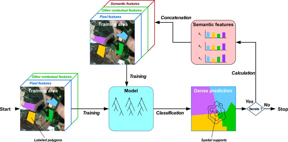
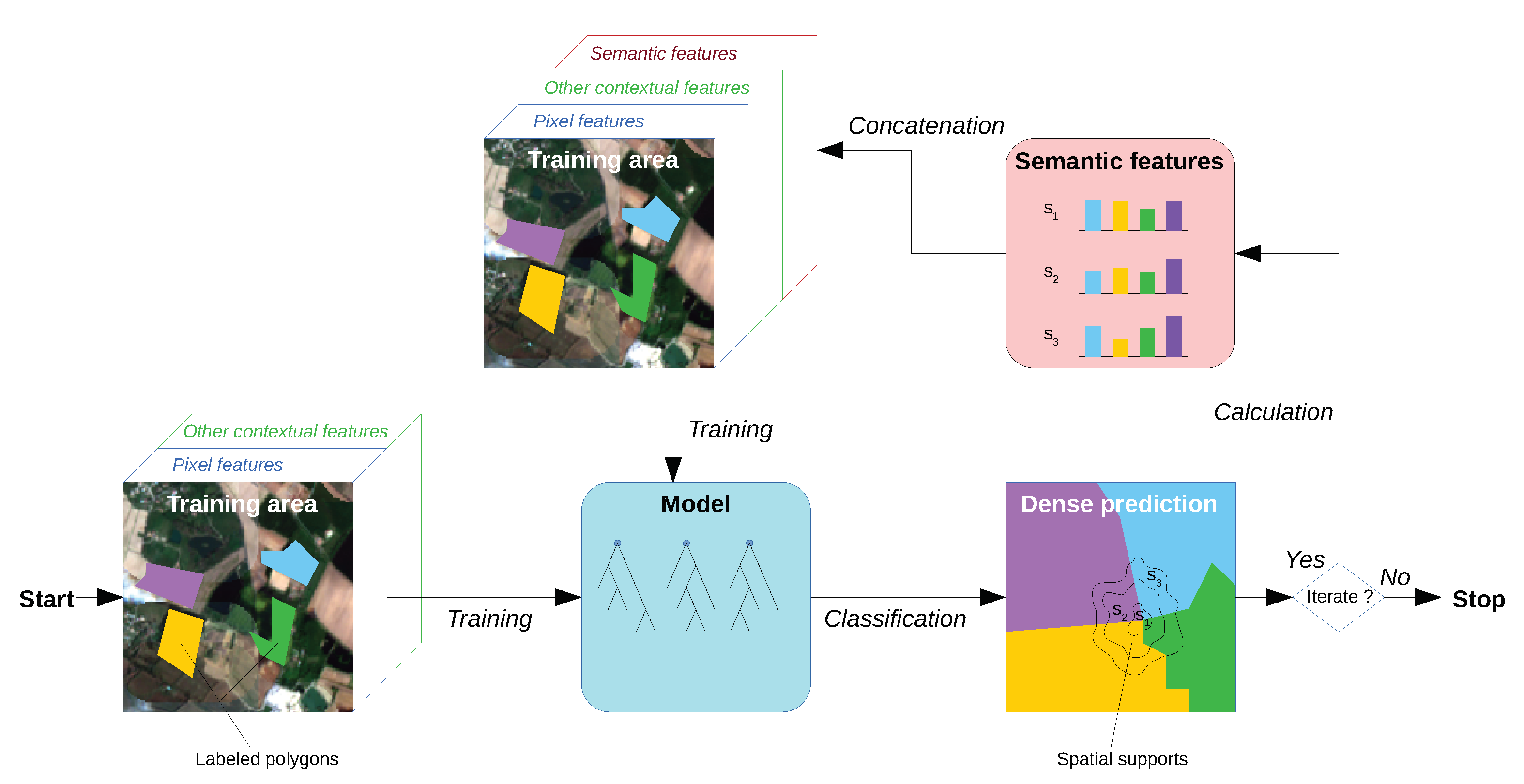
2. The Histogram of Auto-Context Classes in Superpixels process

This study investigates the idea of describing the context of the target pixel using a prior prediction of the class labels of the neighboring pixels. The proposed method is named Histogram of Auto-Context Classes in Superpixels, abbreviated as HACCS. The different aspects and steps of the HACCS process are described in the three following sections.

First of all, Section 2.1 presents the notion of contextual features, namely a group of methods called image-based contextual features. These directly use pixel values or calculate statistics upon the values of neighboring pixels in the image.

Next, Section 2.2 presents stacked contextual classification methods. These first involve applying a prediction, or labeling step to the neighboring pixels, which allows the context to be described in a lower dimensional space than the initial pixel feature space.

Finally, Section 2.3 explains why superpixels were chosen as a spatial support, and how they can be extracted from high-dimensional images which cover wide areas.

2.1. Image-Based Contextual Features

At submetric spatial resolutions, features such as the Scale Invariant Feature Transform (SIFT) [22], the Speeded-Up Robust Feature (SURF) [23], or more recently the Point-Wise Covariance of Oriented Gradients (PW-COG) [24], aim to describe the context of a pixel by characterizing high spatial resolution features, such as sharp gradients and local extrema in the vicinity. This is achieved by extracting so-called keypoints, which are meant to characterize the points of interest in the image, and should help describe its content. This way, a pixel can be characterized by statistical information regarding the keypoints in its surroundings.

Another popular contextual feature for the classification of High Spatial Resolution (HSR) imagery is the Extended Morphological Attribute Profile (E-MAP) [25]. This contextual feature is based on a series of mathematical morphology operations, namely closing and opening by reconstruction. The E-MAP describes the scale at which a pixel in the image is distinguishable from its neighborhood, and whether the pixel is generally lighter or darker than its surroundings. Other morphological attributes also describe geometrical properties such as elongation and squareness.

The issue with the previously mentioned features (SIFT, SURF, PW-COG, E-MAP), and with many other image-based features that are not mentioned here, is that they describe the spatial support in a very high dimensional space. For this reason image-based contextual features have limited applicability to land cover mapping based on high-dimensional imagery.

2.2. Local Class Histograms as a Contextual Feature

Most image-based features (SIFT, SURF, E-MAP) describe the spatial support in a dimension proportional to the number of pixel features, which is prohibitive for application on multi-spectral time series or hyperspectral imagery, for example. For this reason, unsupervised dimension reduction methods, for instance Principal Component Analysis (PCA), Independent Component Analysis (ICA), have been used before in studies on hyperspectral imagery [26,27,28]. However, there is no theoretical guarantee that the relevant information for distinguishing the target classes is contained in the dimensions or linear combinations of dimensions with the highest variability in the data set.

Ideally, the reduction in dimensions should be guided by the classification problem at hand. This is the motivation behind stacked classification methods, which are based on a projection of the high-dimensional pixel features into a lower dimensional label space, using either a supervised classification scheme, or an unsupervised clustering technique.

For instance, the Bag of Visual Words (BoVW) method [29], consists in applying k-means clustering to a set of SURF keypoints, in order to extract a dictionary of so-called visual words. These represent different spatial features, such as corners or a local extrema. Then, the histograms of these visual words are calculated within a spatial support to be used as contextual features. The histogram can also be calculated on an entire image, for instance for image classification or for image matching [30]. An unsupervised approach is used because an extensive nomenclature to characterize each of the low level classes in the image is impossible to obtain. Another reason for using clustering is that keypoint features and texture features often present very large dimensions, and clustering reduces the dimension of the contextual feature to the size of the visual dictionary.

Stacked classification methods can also use a supervised labeling, as is done in [31], where an RF is used to classify the keypoints, and the scores from the various trees in the RF are then used by a SVM classifier. Here, in order to preserve the applicability to high-dimensional imagery, keypoint extraction methods are avoided.

Stacked contextual classification methods use the fact that the systematic errors of a pixel-based classifier can help characterize context-dependent classes. A pixel-based prediction is made with no knowledge of the context, and therefore contains certain predictable sources of errors, which can be learned in the successive iterations. For example, in land cover mapping, the combination of any artificial class and vegetation class in the same histogram serves as a strong indicator of the presence of discontinous urban cover.

The idea of using the result of a supervised classification to provide contextual information as an input to a classification model is essential to the Conditional Random Field (CRF) methods [32,33]. These methods involve using the estimated class-conditional probability density functions in a $3\times 3$ neighborhood surrounding each pixel to build a context-aware model by minimizing energy functions to enforce coherence with the transitions observed in the training data set.

Another group of methods, known as the Semantic Texton Forests (STF) [34], involves using a great number (millions) of features to generate the splits of the Random Forest. These features are simple functions of raw image pixels within a sliding window around the target pixels: either the raw value of a single random pixel, or the sum, difference, or absolute difference of a random pair of pixels. The optimization of the purity criteria guarantees the use of relevant features that best split the training data. Random pixels and pairs of pixels in the neighborhood provide a contextual characterization, in a way similar to how the CNNs consider the different combinations of neighboring pixels through convolutions. In a second step, the histogram of the tree responses and the histogram of the split nodes are calculated in a neighborhood (sliding window [34], or object [35]), and these are used as features for the final classification.

This is similar to the Auto-Context method [36,37]. In these studies, each pixel is classified using a number of image-based features, namely, color and texture features. While the initial classification is coherent, it lacks fine geometrical details in corners, and has the tendency to blur out sharp elements. In their study, the authors use successive iterations of classification using the same classifier and training data, but add supplementary features based on the predictions of the previous iteration. Specifically, the mean of the vector of class probabilities provided by the classifier, in several regions surrounding the pixel is used. As there are only two classes, this represents a very low total number of extra features, which allows a large number of different neighborhoods to be considered simultaneously, and for the pixel and image-based features to be preserved throughout the process. Selecting the shape and location relative to the target pixel of these neighborhoods carefully allows different aspects of the problem to be learnt by the classifier, for instance, spatial relations between classes, or relative positional information. The authors concluded that applying the Auto-Context algorithm several times refined the details of the geometry and improved the quality of the output classification. In fact, a large number of iterations was not seen as necessary, as the authors observed no more notable changes in the results after 5-6 iterations. This means that the process is light and fast, and potentially applicable to classification over wide areas with high-dimensional imagery.

The STF and Auto-Context methods address a similar problem as the one encountered in land cover mapping over wide areas, namely, the difficulty of classifying context-dependent areas while preserving the sharp corners and fine elements, on a large dimensional data set. Nonetheless, there are several differences between these methods and the HACCS process.

First of all, a normalized histogram of the predicted labels is used rather than the output probability vector of a soft labeling classifier, in a similar way to the histogram of clusters used in the BoVW features. Second of all, rather than using sliding window neighborhoods as in [34,38,39], or more recently in [40,41], superpixels are used as spatial support to calculate the class histograms.

Figure 1 shows the different steps of the HACCS process. By using pixel features, optionally in combination with other contextual features, an initial classification model is trained. This model is then used to achieve a first dense classification of the image. Once all of the pixels in the image are labeled, the histogram of these predictions is calculated in each neighborhood, and used as a contextual feature. In the HACCS process, image-based features can optionally be used to generate a more accurate estimation of the first dense classification map. They can be useful for improving the quality of the first classification, and for providing complementary contextual descriptors to the histogram of classes. These optional features are represented by the green box labeled “Other contextual features” in Figure 1.

The methods cited above can be described by five properties, given in the following list.

• The density of the initial prediction: certain methods predict the class or cluster of keypoints, whereas others use every single pixel in the image.
• Supervised or unsupervised prediction: some methods prefer the use of clustering rather than supervised classification for the initial prediction.
• The contextual features, or lack thereof, used for the initial prediction: the first prediction can be pixel-based, or can already be based on the use of pre-selected contextual descriptors.
• The number of iterations: certain methods stop at the second prediction, while others use successive predictions to improve the classification in an iterative way.
• Adaptive spatial support. The definition of the context can be a sliding window, or an adaptive spatial support.

Table 1. Five main properties of methods that use a label prediction to include contextual information in a classification scheme. The Histogram of Auto-Context Classes in Superpixels method has the potential to verify all five of the properties.

Method	Dense	Supervised	Initial Context	Iterative	Adaptive
CRF [32]	X	X		X
BoVW [29]			X
Stacked [42]	X	X		X	X (object)
Stacked [31]		X	X	X
STF [35]	X	X	X		X (object)
STF [34]	X	X	X
Auto-Context [36]	X	X	X	X
HACCS	X	X	optional	X	X (superpixel)

shows the characteristics of the different methods that were cited previously. Clearly, the nomenclature of the different methods is not very well defined, as they originate from a variety of backgrounds and applications. None of the methods possess all five of the characteristics. Table 1 also shows that the the HACCS method can in some cases bear all five of these properties.

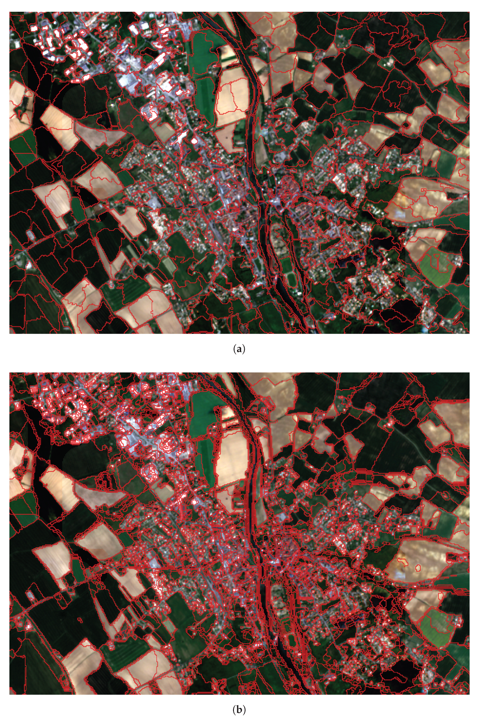
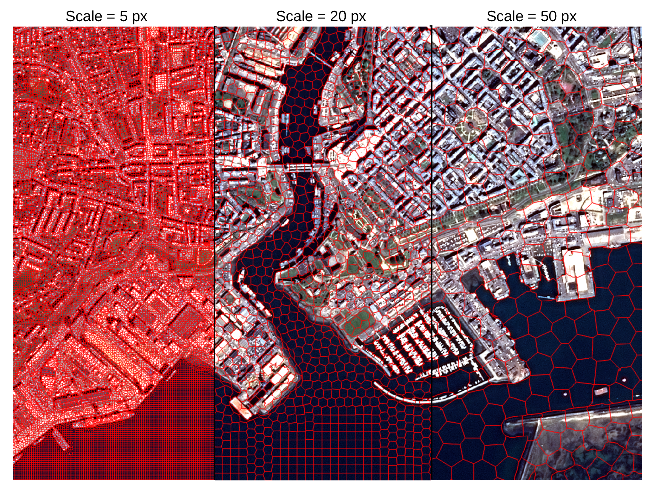
2.3. Multi-Scale Superpixels as Spatial Supports

The choice of which spatial support to use to calculate the histogram of the class labels is not a simple one. Two commonly used spatial supports used for calculating contextual features are sliding windows and objects [19].

Previous studies on the geometric precision of land cover mapping have shown that the use of a sliding window neighborhood with a so-called unstructured feature can increase the risk of blurring out high spatial frequency image features [43]. Unstructured features do not take into account the spatial arrangement of the pixels in the neighborhood. Other examples of unstructured features are the sample mean and variance. In fact, this phenomenon is observed on experiments on the Sentinel-2 and SPOT-7 datasets, shown in Section 4.

The other popular spatial support is the object, which is the result of an object segmentation method such as Mean Shift [44], or Region Merging [45]. Figure 2b shows that in highly textured areas such as urban areas, the Mean Shift segmentation algorithm fails to provide segments containing diverse pixels. Therefore, a different type of segmentation is used here: superpixel segmentation. The algorithm used in this study, known as Simple Linear Iterative Clustering, or SLIC [46], aims to provide segments that exhibit homogeneous features, but are also similar in size, and have a relatively compact shape, as is shown in Figure 2a.

This algorithm is also very fast, and can be applied to remote sensing imagery over wide areas, using the scaling method described in [47]. The size of the grid at the first iteration of the SLIC algorithm is a parameter which is set manually, and which conditions the average size of the superpixels in the final segmentation. This parameter is referred to as the scale of the superpixel segmentation. The scale of a superpixel segmentation can be seen a characteristic diameter, in other words, the square root of the average area of the segments. This parameter gives an indication of the average distance at which contextual information is considered.

The choice of which scales to use depends on the application, in particular, which context-dependent classes are targeted, as well as the spatial resolution of the images. Initial experiments on the HACCS process indicate that using histograms in several scales of superpixels is beneficial compared to using only one. Indeed, it seems reasonable that a multi-scale description of the neighborhood would be useful for characterizing context-dependent land cover classes.

The scale of the superpixels is a parameter of the HACCS process, which can be selected according to a priori knowledge of the target classes, through experimentation, or both.

3. Deep Convolutional Neural Networks

This section details two types of Convolutional Neural Network (CNN) that were recently used to classify land cover: patch-based networks and fully-convolutional networks.

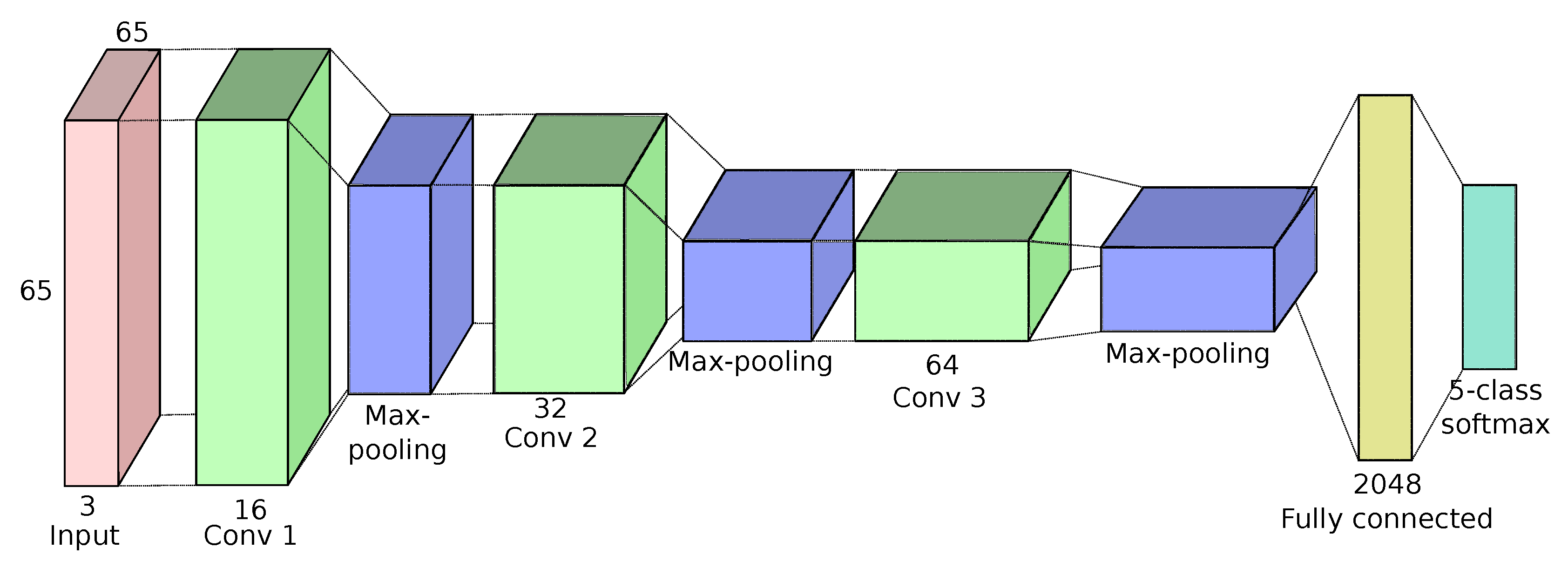
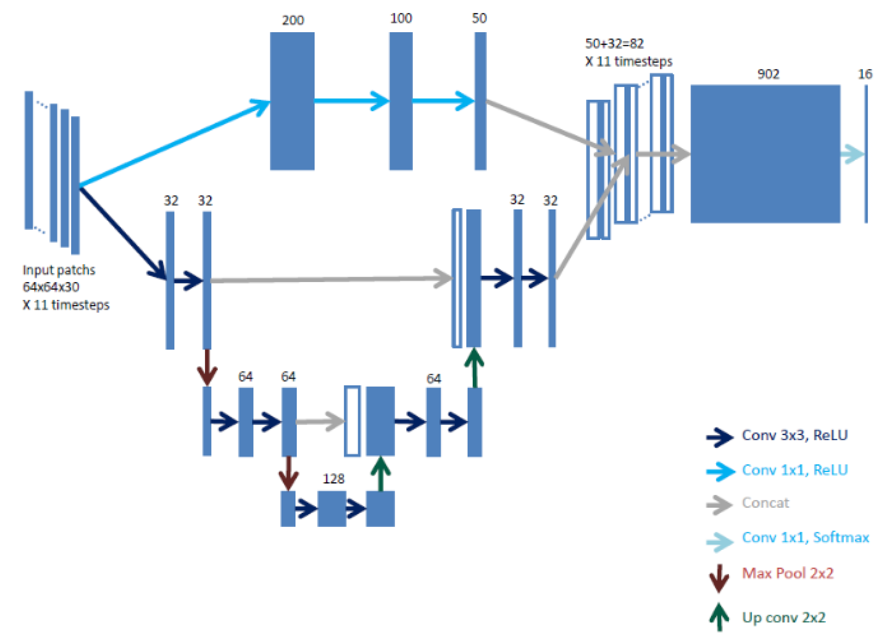
3.1. Patch-Based Network

Patch-based methods involve taking a standard CNN architecture such as the ones applied on the ImageNet database [11], and considering that the output label, which was originally meant to describe the entire patch, is assigned only to the central pixel of the patch. This way, all of the pixels in the image can be labeled by applying the network to a window around each pixel, like a sliding window. Furthermore, this is adapted for sparsely labeled training data, where each training sample is a labeled pixel. This allows for existing network architectures originally used for image classification to be re-used to achieve a dense classification, and therefore allows neural networks to be applied to land cover mapping [48,49]. Recently, a patch-based network was successfully applied on a five-class land cover mapping problem, including context-dependent classes such as roads and urban cover, which are commonly confused by pixel-based classifiers [50]. Figure 3 shows the relatively simple network architecture, which is composed of three stages of convolution and max-pooling, followed by a fully connected layer.

For training a patch-based D-CNN, training patches are sampled throughout the labeled polygons. Examples of such training patches are shown in Figure 4.

3.2. Fully Convolutional Networks

The other way to use Convolutional Neural Networks to achieve dense classification involves combining a series of convolutional and max-pooling layers to a series of deconvolution and unpooling layers, to assign a label to each pixel in the patch. For this reason, it will be referred to as the fully-convolutional network in this paper. This is the idea behind networks like Seg-Net, [51] and U-Net [6,52]. This way, entire patches of the image can be classified without the need to pass through the whole image, which means that fully convolutional neural networks are usually faster than their patch-based counterparts. These methods are usually applied in conjunction with dense training data, but several recent studies have shown that this architecture can also be applied to problems with sparse training data. In [53], the authors propose a Fine Grained U-Net architecture (FG-Unet), shown in Figure 5, which is a slightly modified version of the classic U-Net architecture, particularly to deal with the issue of sparse training data. Usually, the loss function $\mathcal{L}$ is calculated by comparing the output of the last layer of the network, which contains the label predictions, to the densely labeled training patch. When the training data are sparsely labeled, the adapted loss function ignores the unlabeled points, as is shown in Equation (1), where $y_{true}$ and $y_{pred}$ respectively designate the ground truth and predicted vectors of size $class\_nb$. Moreover, a weighted average is made using the parameter $weigh{t}_k$ over the various classes, in order to provide more weight to classes with a low number of training points, to deal with imbalances in the class priors. Figure 6 shows an extract of the training polygons in order to illustrate the sparse spatial distribution of the data set.

$$\mathcal{L}=\sum _{pixels}\sum _{k=1}^{class\_nb}weigh{t}_k·y_{tru{e}_k}·log\left(y_{pre{d}_k}\right)$$

(1)

Secondly, a weight-sharing scheme is employed on the convolutional layers, in order to limit the size of the initial layers. The data set is a time series 33 of multi-spectral images containing 10 bands each, as is shown in Section 4.2. The large number of dimensions in the input data is necessary, however, if no precautions are taken, it can create very large networks that are more difficult to optimize. A third adaptation to the U-Net architecture is made, in order to deal with the issues of blurring in the output maps. This consists in connecting a series of 1 × 1 convolutional layers to the fully-connected layers in the deepest part of the network. In other words, this is equivalent to adding a pixel-based classification of the time series at full resolution to aid in the decision.

3.3. Issues with Sparse Data

Geometric degradation, in other words, the smoothing of sharp corners and of small elements in the classification map, is a recurrent observation in several recent studies evaluating the use of Deep Learning architectures to achieve dense classification with a sparse data set. In [54], a patch-based network is used to classify crops using a combination of Landsat-8 and Sentinel-1 time series. While the CNN approach outperforms the pixel-based RF, the authors note that some small objects are misclassified, and the sharp corners appear rounded in the final result. Similar misclassifications are also observed in hyperspectral image classification, when using a patch-based network based on Auto-Encoder features [55].

This phenomenon is rarely considered by studies that apply CNN models with dense training data on toy problems, but is a real issue for land cover mapping. Indeed, when dense training data are available, the use of fully convolutional networks can provide land cover and land use mapping with high context-dependent class recognition rates and spatial precision, as is shown in [56,57].

The reasons for this geometric degradation are difficult to assess precisely, but a review of the current literature, and an analysis of the way CNN models work, suggest that this phenomenon may be linked to the use of sparse training data.

The CNN aims to optimize both the feature extraction step, and the classification step, in an end-to-end fashion. In other words, the training data drive both the selection of which contextual features to use, and how to use them properly to achieve a precise classification. This is the case for both the patch network and the fully convolutional network, presented previously.

However, by basing the feature extraction step entirely on the training data, problems may appear when these data do not contain a sufficient quantity of points to correctly characterize certain elements of the problem. Indeed, the success of any data-driven method like CNN is very dependent on the quality of the training data, in other words, how well the training data represent the desired output. This leads to the common conception that training a deep neural network requires a large amount of training data, which true in most cases, especially for complex problems. For this reason, in practice, several applications using CNN models increase the number of training samples by applying data augmentation techniques such as rotations and other such transformations. However, having a large amount of training data does not always mean that the Deep Learning approach will be successful. Indeed, the training data must be sufficiently rich to cover the most important aspects of the classification problem in the first place.

Unfortunately, in the case of operational land cover mapping, the training data are very rarely densely distributed across the image, because they usually come from several different sources, which combine on-ground measurements with human photo interpretation [5,50]. This implies that the fine grained-geometry, i.e., the specific spatial arrangement of the classes is absent from the training data set. Moreover, the labeled points are generally concentrated in the center of the objects, and rarely on the edges or in the corners.

Patch-based CNNs may encounter issues linked to an insufficient amount of training points in sharp corners and along the object boundaries, which can reduce the spatial precision of the labeling. The high-level decision layers are situated after several pooling layers which reduce the spatial resolution, meaning that a geometrically precise decision can be difficult to obtain. For this reason, fully convolutional networks like U-Net introduce skip connections, which pass full resolution information to the deep layers of the network.

Generally speaking, if a neural network has never been trained on a labeled pixel that lies near the boundary between two classes, it might produce a result with an edge displaced towards one of the two classes. In practice, this often translates in a degradation of the high spatial resolution elements in the output classification. Sharp corners are rounded, and fine elements are either thickened, or entirely erased. The lack of dense training data also explains the speckle-like label noise observed near object boundaries in [50]. Simply put, the areas that lack a sufficient description in the training data contain a large number of confusions.

4. Experimental Results

This section provides the experimental results of this study, which compares the abilities of the HACCS process and the CNN approach to produce land cover maps with high degrees of thematic and geometric accuracy, in context-dependent areas. To provide general results and insights for different problems, experiments on two land cover mapping problems with different spatial, temporal and spectral resolutions are proposed. This is done in order to evaluate the performance of the HACCS method in a variety of cases, to show how, like the CNN approach, it can be adapted to different dense image classification problems.

Section 4.1 describes the two experimental setups that were used in order to provide a comparison between the proposed method, HACCS, and the Convolutional Neural Networks. Section 4.2 and Section 4.3 show the results of this comparison, respectively on the Sentinel-2 time series and on the SPOT-7 classification problems.

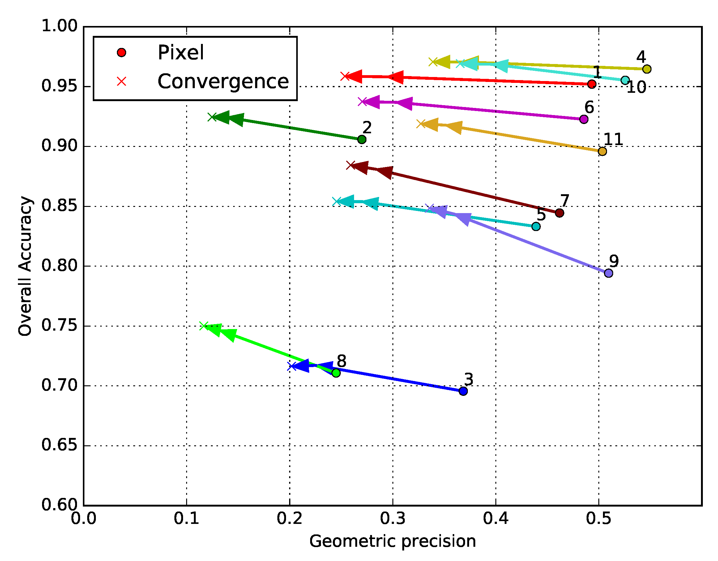
4.1. Evaluation Metrics

The evaluation of the classification results is first of all based on the usual statistical measurements, Overall Accuracy (OA), Kappa, and F-scores. However, experience has shown that these indicators can be misleading when evaluating the dense classification of an image, in the absence of dense validation data. Indeed, the methods that are tested here include contextual information, which is known to have an impact on the geometry of the classification result, compared to the pixel-based approach. This is particularly visible along object boundaries and in the corners and fine elements, as is visible in the results, shown in Figure 18a,b. Sparse validation data do not contain many of these sensitive areas. In other words, they are biased towards the most common samples, which are concentrated near the center of the image objects. Therefore, errors in corners and fine elements have a low influence on the overall metrics, and can be overshadowed by other positive effects like the removal of isolated pixels.

There exist several metrics that aim to quantify the quality of the geometry of a classification map, when dense validation data are available. For instance, the Hoover metrics [58], measures aspects like the degree of oversegmentation, undersegmentation, or noise present in the result, with respect to the reference objects. Intersection Over Union (IoU) [59], is also commonly used, although it presents the same issues as OA and Kappa, as it measures a score averaged over the pixels of each object. Otherwise, there are categorical measurements, based on the class precision in various geometrical elements like corners, edges, centers, [60,61], however these require a prior knowledge of the localization of the corners, edges, and centers, which is unavailable due to the sparsity of the reference data.

For these reasons, the Pixel Based Corner Match (PBCM), developed in [43] was used to evaluate the quality of the land cover maps, as it does not require a dense validation set. The PBCM metric uses a pixel-based predicition to extract corners in the densely classified image, called $C_{ref}$, which are a key element to evaluate the quality of the geometry. These corners are compared with the set of corners detected in the contextual classification, noted $C_{test}$. The metric is based on the number of matching corners in the two classifications, with respect to the initial number of corners. This measures how many of the corners disappear from the result, or are displaced due to a geometrical degradation. The set of matching corners, $C_{match}$, is defined as the corners in the contextual classification that are within a small distance (for instance, 1 pixel) from at least one corner in the pixel-based classification, as is shown in Equation (2), where $dist(x,y)$ is the standard Euclidean distance, and t is a threshold parameter.

$$C_{match}=\{x\in C_{test}\mid \exists y\in C_{ref},dist(x,y)\le t\}$$

(2)

Then, the geometrical precision score m can be written as in Equation (3), where $Card\left(C\right)$ is the number of elements in the set C.

$$m=\frac{Card\left(C_{match}\right)}{Card\left(C_{test}\right)}$$

(3)

Moreover, to provide statistically significative results, each classification was run a total of 10 times with different samplings of the training and validation data sets. The average and standard deviation of the scores are used as metrics for the analysis. The sampling strategy involves splitting the training and testing data sets on a polygon level, in order to avoid biases between the two data sets [5].

4.2. Sentinel-2 Time Series Classification Problem

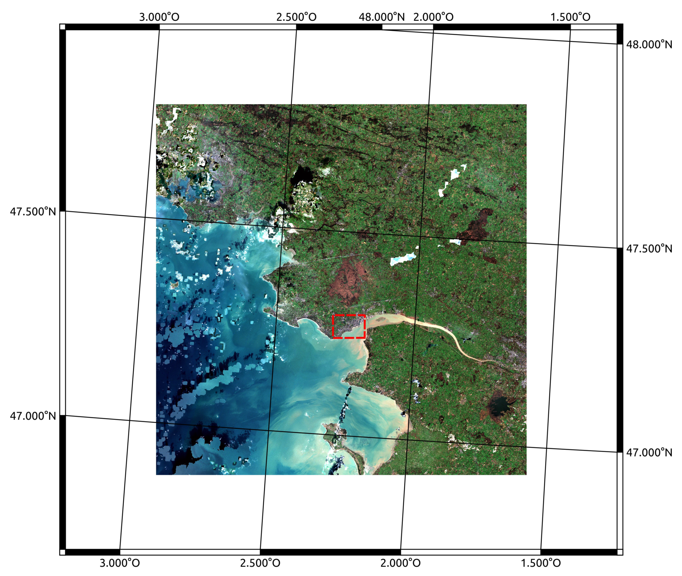
4.2.1. Description of the Sentinel-2 Data Set

The first experimental case that was studied is a 17 class problem, based on high spatial resolution Sentinel-2 multi-spectral time series. This data set contained 11 different 110 × 110 km areas across France that covered a variety of landscapes and eco-climatic areas. The methodology for generating time series adapted for supervised classification was identical to the approach developed by [5]. Figure 7 shows the position of the 11 tiles on a map of the metropolitan French territory.

The training data for this classification problem come from various sources:

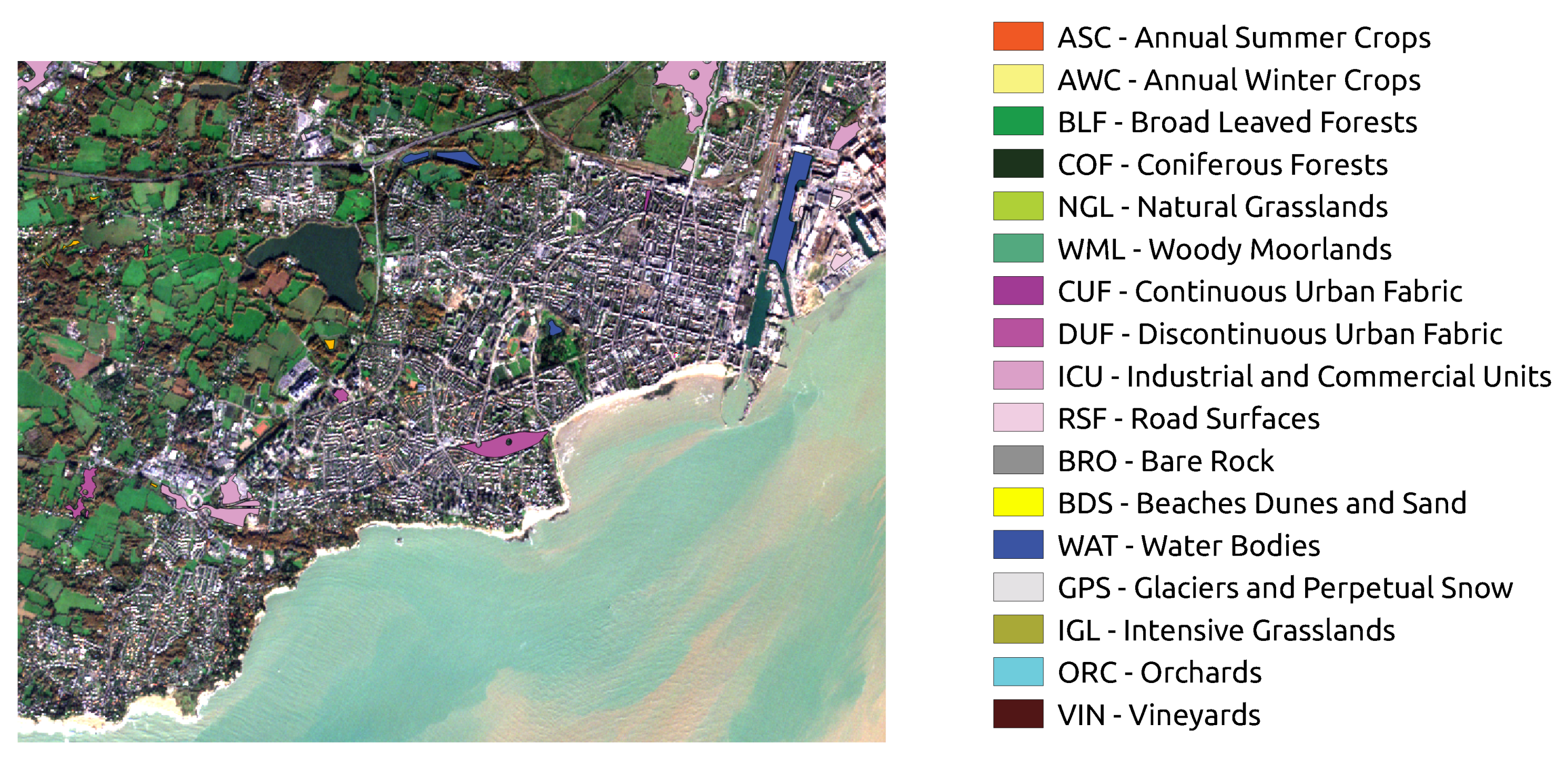
• Corine Land Cover (CLC) [62] is based on manual photo-interpretation, and is updated every six years. It contains a rich description of the many land cover elements, with a nomenclature of 44 classes. This data base is used for the perennial classes: water, beaches, and bare rocks.
• Urban Atlas (UA) [63] covers all cities with over 100,000 inhabitants, and is updated every six years, like CLC. It contains 17 classes describing different levels of urban density, as well as other urban features like construction sites, sports and leisure sites. Urban Atlas is used as a reference for the four urban classes: continuous urban fabric, discontinuous urban fabric, industrial and commercial units, and road surfaces.
• National Topo Data Base (BD Topo) [64] is a regularly updated data base made by the French National Geographical Institute (IGN). The forest database describes the main woody cover classes (woody moorlands, broad-leaved and coniferous forests). The urban data base gives the outline of buildings, but does not provide an indication of the urban density.
• Graphical Parcel Registry (RPG) [65] is another product of the IGN which describes arable lands based on a graphical declaration system from the farmers. It contains an up-to-date description of the main agricultural classes.
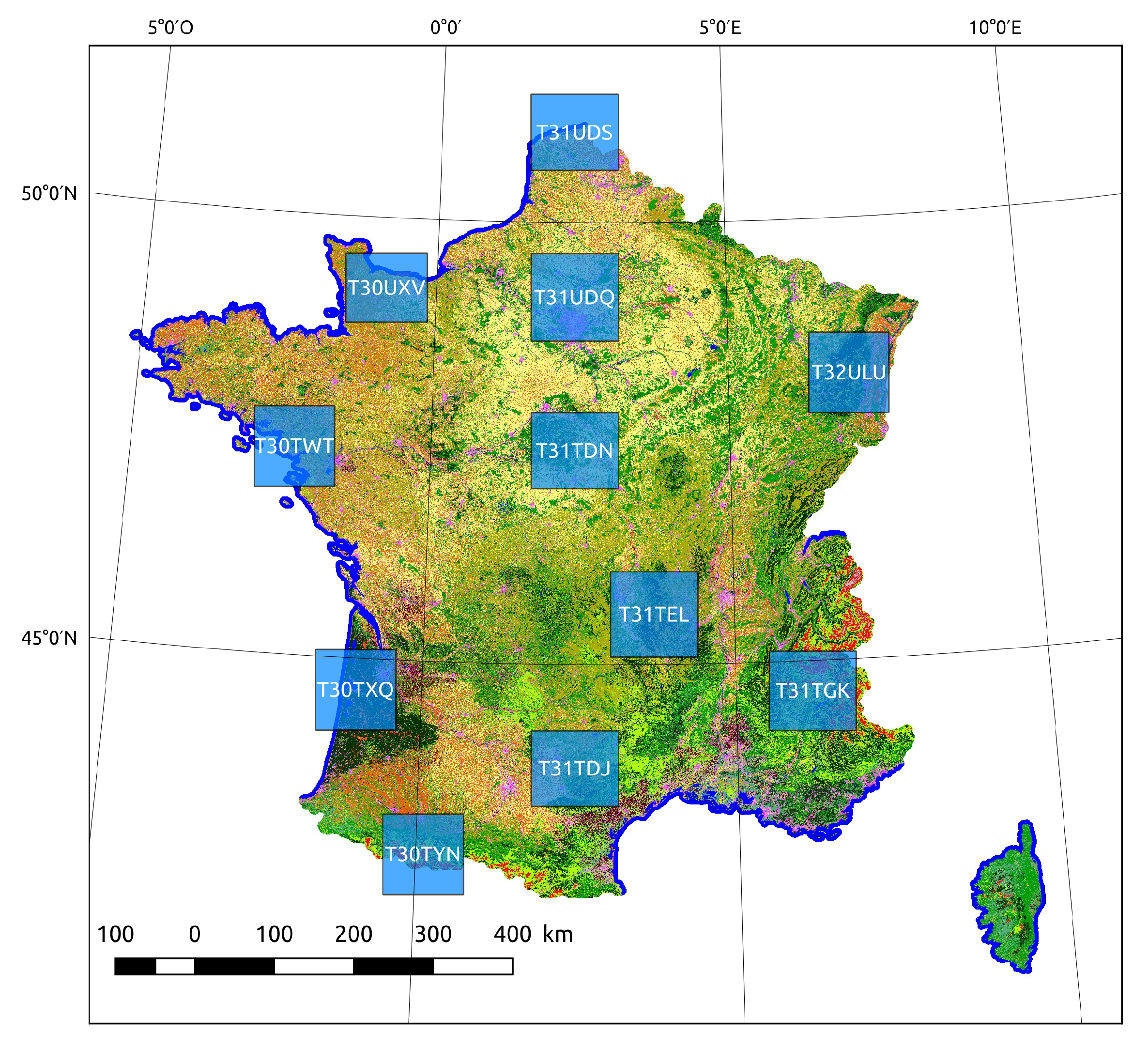
• Randolph Glacier Inventory (RGI) [66] contains a worldwide description of the glaciers, and is updated every one or two years.
  The number of training samples taken for each tile is shown in

  Table 2. Number of samples taken for training on the various tiles. The meaning of the three letter class abbreviations is given in Figure 6. To preserve balance between the classes, a maximum number of 15,000 samples was used.

  Name	T30TWT	T30TXQ	T30TYN	T30UXV	T31TDJ	T31TDN	T31TEL	T31TGK	T31UDQ	T31UDS	T32ULU
  Index	1	2	3	4	5	6	7	8	9	10	11
  ASC	15,000	15,000	15,000	15,000	15,000	15,000	15,000	2576	15,000	15,000	15,000
  AWC	15,000	2484	9271	15,000	15,000	15,000	15,000	14,149	15,000	15,000	15,000
  BLF	15,000	15,000	15,000	15,000	15,000	15,000	15,000	15,000	15,000	15,000	15,000
  COF	15,000	15,000	15,000	14,575	15,000	15,000	15,000	15,000	15,000	1541	15,000
  NGL	6496	0	15,000	0	15,000	732	15,000	15,000	1220	1377	15,000
  WML	15,000	15,000	15,000	7975	15,000	15,000	15,000	15,000	15,000	8468	8641
  CUF	12,262	15,000	3271	14,154	1841	2247	15,000	373	15,000	15,000	15,000
  DUF	15,000	15,000	15,000	15,000	15,000	15,000	15,000	13,739	15,000	15,000	15,000
  ICU	15,000	15,000	14,706	15,000	15,000	15,000	15,000	5679	15,000	15,000	15,000
  RSF	3761	15,000	1674	2307	1029	2803	15,000	1214	15,000	12,900	9203
  BRO	0	0	15,000	406	0	0	80	15,000	0	0	0
  BDS	3729	15,000	0	3811	0	1687	0	14,315	0	3778	0
  WAT	15,000	15,000	12,511	15,000	15,000	15,000	15,000	15,000	15,000	15,000	15,000
  GPS	0	0	1978	0	0	0	0	15,000	0	0	0
  IGL	15,000	15,000	15,000	15,000	15,000	15,000	15,000	15,000	15,000	15,000	15,000
  ORC	1499	345	37	2205	2171	809	202	6122	4935	578	695
  VIN	4406	15,000	89	0	15,000	2784	917	78	0	0	3433

  . Each tile contains quite different class proportions, which implies the evaluation is performed on a variety of different situations, in order to address the particularities of some of the minority classes that are only present in certain regions.

In order to be coherent with the validation of the FG-Unet results made by [53], validation scores using the full extent of the testing data are shown in these experiments. The class distributions of the testing data on the 11 tiles is shown in

Table 3. Number of samples taken for validation on the various tiles.

Name	T30TWT	T30TXQ	T30TYN	T30UXV	T31TDJ	T31TDN	T31TEL	T31TGK	T31UDQ	T31UDS	T32ULU
Index	1	2	3	4	5	6	7	8	9	10	11
ASC	186,084	112,870	39,577	111,140	61,063	66,908	127,364	2576	109,349	32,778	114,279
AWC	170,839	2484	9271	169,424	132,590	368,659	186,646	14,149	1,079,411	151,941	74,096
BLF	65,003	92,320	137,546	47,169	143,008	438,458	352,358	143,659	429,562	56,820	296,402
COF	86,055	3,406,794	123,960	14,575	209,091	99,486	1,571,267	864,432	102,111	1541	985,948
NGL	6496	0	335,427	0	58,593	732	31,962	825,736	1220	1377	24,063
WML	112,019	102,667	184,257	7975	64,156	20,671	111,814	307,237	27488	8468	8641
CUF	12,262	34,133	3271	14,154	1841	2247	39,067	373	287,388	15,081	15,947
DUF	197,925	368,733	25,559	50,932	25,543	31,550	233,471	13,739	1,035,603	82,494	107,867
ICU	178,134	281,722	14,706	50,771	20,237	39,447	148,008	5679	841,308	108,103	79574
RSF	3761	22,572	1674	2307	1029	2803	19,327	1214	67,095	12,900	9203
BRO	0	0	231,491	406	0	0	80	77,756	0	0	0
BDS	3729	112,848	0	3811	0	1687	0	14,315	0	3778	0
WAT	4,650,221	6,458,981	12,511	1,959,898	58,971	80,282	46,231	34,065	84,697	1,894,379	44,049
GPS	0	0	1978	0	0	0	0	54,664	0	0	0
IGL	249,625	22,112	109,417	301,560	87,286	89,923	761,126	117,134	150,013	40,845	156,124
ORC	1499	345	37	2205	2171	809	202	6122	4935	578	695
VIN	4406	52,594	89	0	17,135	2784	917	78	0	0	3433

. This provides a more realistic estimation of the overall accuracy in the sense that it contains many more points, although the majority classes have a stronger influence on the score than the minority classes. Fortunately, the F-scores are relatively independent of the class prior density distributions, and are therefore frequently used in the performance analysis.

The area of interest that is used for visual map analysis in Section 4.2.2 is the city center and harbor area of Saint Nazaire. Figure 8 shows this area within the T30TWT tile. The juxtaposition of continuous, discontinuous and industrial areas along with sharp geometrical features along the water make it an interesting study area.

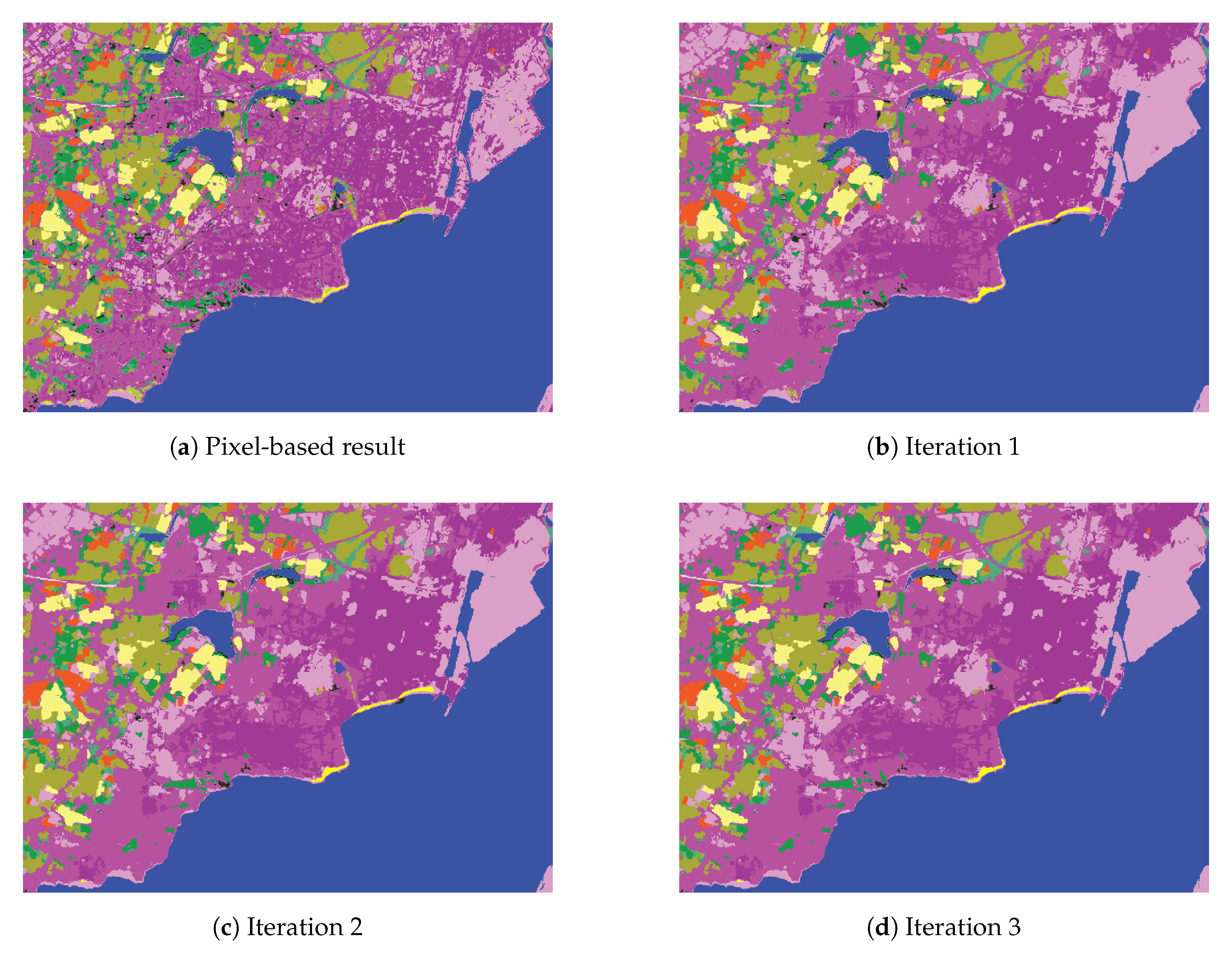
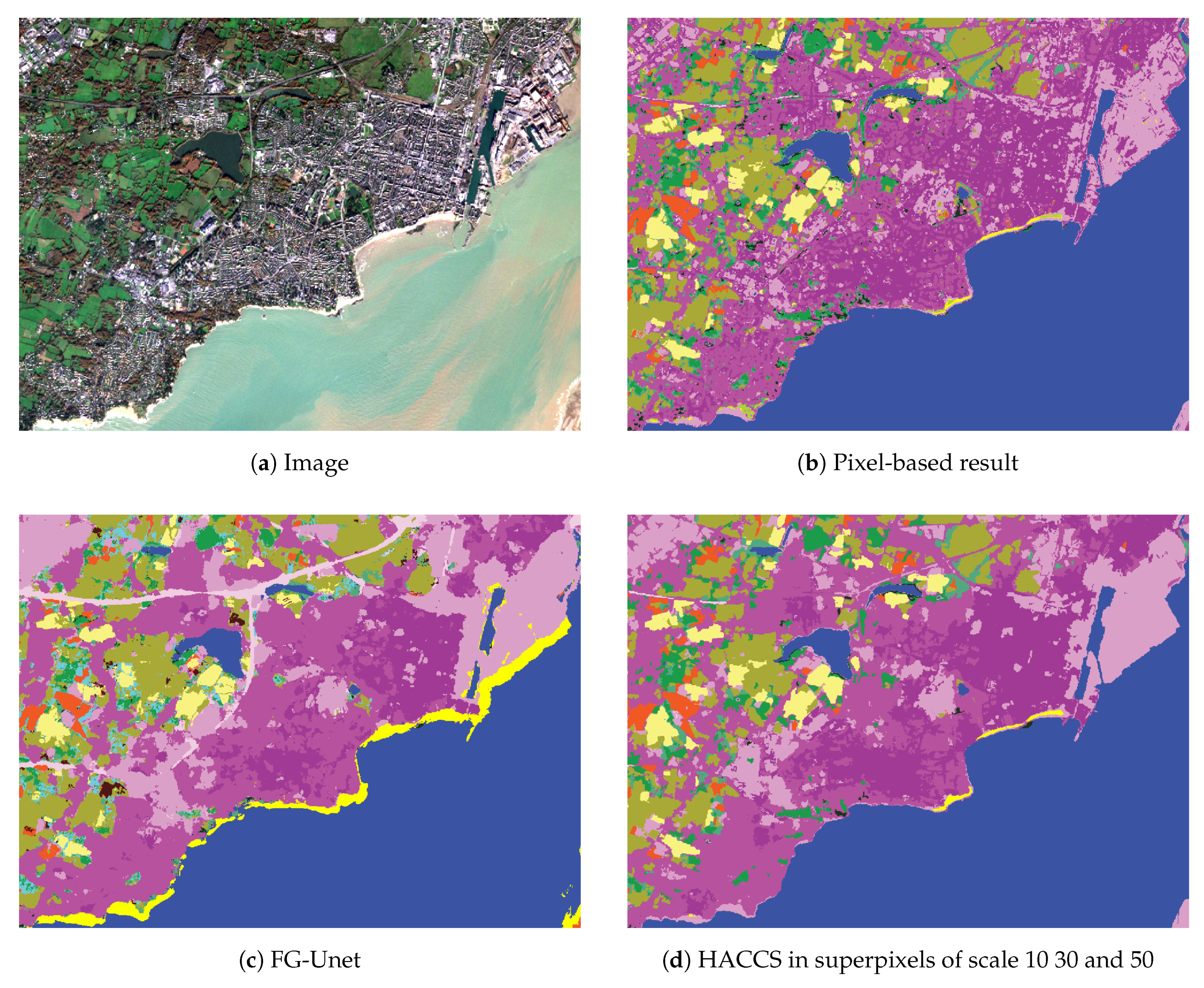
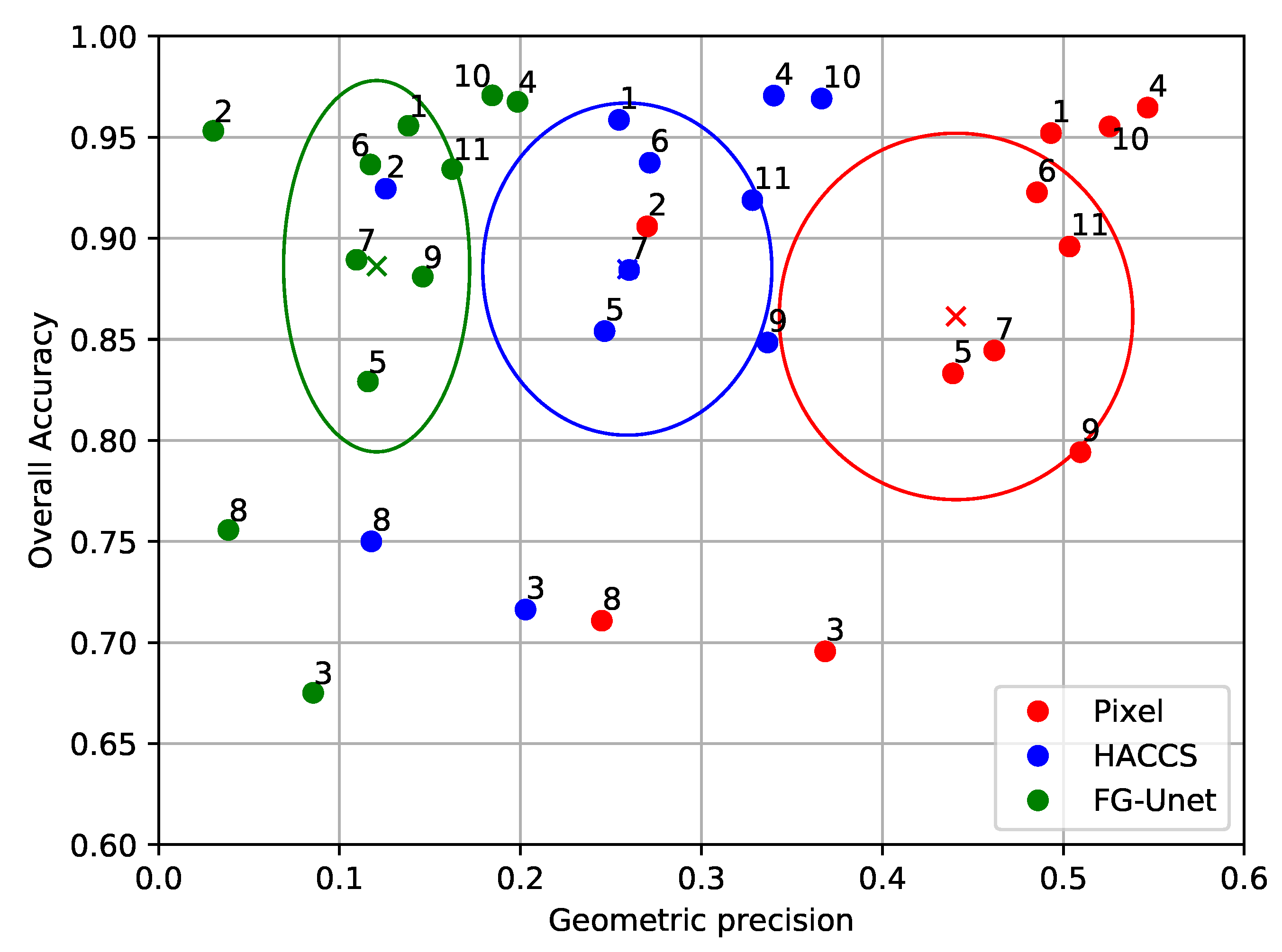
4.2.2. Results on the Sentinel-2 Problem

In these experiments, the Random Forest classifier was applied with a total of 100 trees, using a maximal depth of 25. These parameters were found to be sufficient for this problem by [5], and were therefore not changed for this study. Figure 9 shows the classification maps of the first iterations of the HACCS process. To produce the result of iteration 1, a pixel-based classification result was used to estimate the class histograms in several scales of superpixels, as is explained in Section 2. Then, this result was used to update the histograms, which generated a new iteration. The majority of the changes occurred at iteration 1, when contextual features were included for the first time. The most obvious effect was the smoothing of the classification result, in other words, the removal of isolated pixels. This regularization eliminated many of the pixel-based classification errors. Moreover, the distinction between the four urban classes became more and more accurate; there was a clear separation between the industrial area surrounding the harbor, the dense urban area in the city center, and the discontinuous urban area near the periphery. On the downside, the roads network was not entirely recognized, and some of the vegetation surrounding urban areas was falsely classified as discontinuous urban fabric.

The impact of the iterations on the overall accuracy and geometric precision is shown in Figure 10, which plots these two metrics across three iterations of HACCS, for the eleven tiles. The arrows show the rapid progress of the performance indicators, which converged within very few (2-3) iterations. This is also visible in Figure 9; the classification results in Figure 9c,d are almost identical. Generally speaking, the HACCS process had the effect of increasing the overall accuracy of the classification with respect to the pixel-based classification, regardless of the tile on which it was applied. This also came at the cost of a decrease in PBCM, as some of the corners were lost or displaced. This figure also shows that tiles with a lower initial overall accuracy showed stronger improvements than tiles that were already relatively well classified. This is explained by the fact that these difficult tiles most likely contained larger proportions of context-dependent classes, making them prone to errors when using a pixel-based approach. For example, tiles 31TYN and 31TGK, respectively indexed 3 and 8 in Table 2 covered mountainous areas, and contained significant proportions of the bare rock class, which is very often confused with urban cover. This is also the case for tile 31UDQ which covers the extended urban area of Paris.

For a visual analysis of the results, Figure 11 shows the classification maps generated by the two contextual approaches: FG-Unet and HACCS, compared to the pixel-based Random Forest over the harbor area of Saint-Nazaire. This area is located in the T30TWT tile, in the red dotted rectangle shown in Figure 8. Visually speaking, the HACCS method provided a higher degree of geometric accuracy than the CNN method, as it encouraged label homogeneity in superpixels, which represented parts of physical entities that were present in the original time series. This translated as sharp corners, and other fine details in the classification result. This is coherent with the patterns that were statistically observed over the entire data set.

Next, the per-class performances were analyzed using the F-score metric. The average OA, Kappa, PBCM, and F-scores over the 11 tiles of the experimental data set are shown in

Table 4. Statistical class accuracy of the pixel-based classification, the HACCS process, and of the FG-Unet (CNN) methods, averaged across the 11 Sentinel-2 tiles. The per-class performance is given by the F-score metric, also averaged over the tiles. The method with the highest average score is shown in bold. The 1-$\sigma$ error intervals, calculated across 10 classification runs, are shown for the overall metrics of the pixel-based approach and HACCS. This table shows that HACCS and FG-Unet have a similar overall performance. The CNN approach provides higher recognition rates on three out of the four urban classes (CUF, DUF and RSF), whereas the HACCS process seems to be more beneficial for the natural vegetation and agricultural classes.

Method	Pixel	HACCS	FG-Unet (CNN)
Average OA	86.1% ± 0.12	88.5% ± 0.17	88.6%
Average Kappa	80.6% ± 0.17	83.9% ± 0.23	84.2%
Average PBCM	44.2% ± 0.24	26.1% ± 0.31	11.8%
Summer crop (ASC)	0.929	0.940	0.926
Winter crop (AWC)	0.903	0.899	0.893
Broad-leaved Forest (BLF)	0.843	0.879	0.882
Coniferous Forest (COF)	0.868	0.899	0.843
Nat. Grasslands (NGL)	0.321	0.332	0.244
Woody Moorlands (WML)	0.423	0.469	0.461
Cont. Urban (CUF)	0.330	0.463	0.499
Disc. Urban (DUF)	0.713	0.798	0.835
I.C. Units (ICU)	0.556	0.671	0.660
Road surfaces (RSF)	0.509	0.648	0.666
Bare Rock (BRO)	0.430	0.448	0.423
Beaches, dunes (BDS)	0.469	0.551	0.606
Water bodies (WAT)	0.959	0.954	0.946
Glaciers, snow (GPS)	0.517	0.516	0.718
Intensive Grassland (IGL)	0.768	0.794	0.761
Orchards (ORC)	0.189	0.249	0.214
Vineyards (VIN)	0.464	0.579	0.494

. First of all, it can be noted that as expected, including contextual information into the classification scheme allowed for a significant improvement of context-dependent classes. In terms of statistical class accuracy, the two contextual methods, HACCS and FG-Unet, showed a relatively equivalent performance, with neither method strongly outperforming the other.

The only classes where the pixel-based prediction was generally more accurate were the winter crop and water bodies classes; however, the difference was quite small, and these classes were not a primary focus as they already exhibited very high recognition rates.

However, it is worth noting that the CNN architecture provided generally more precise results on three of the four urban classes: continuous urban fabric, discontinuous urban fabric, and roads, whereas the HACCS method had a strong prediction power for the vegetation classes, like coniferous forests, grasslands (both natural and intensive), orchards, and vineyards. On the two classes where the pixel-based method provided the strongest performance, annual winter crops and water bodies, HACCS provided a slightly more accurate result on average than the CNN approach. Overall, HACCS had stronger results than FG-Unet on 11 out of the 17 classes.

The graph in Figure 12 plots the OA against the PBCM that is defined in Section 4.1, for the different methods and for each different tile. The ellipses show the mean and standard deviation of the two scores calculated across the eleven tiles. This was done to provide an indication of the average performance of the classification over a wide area, as well as the robustness of the different methods to differences in class behavior and class proportions. Each ellipse is centered on the mean of the performance indicator across the eleven tiles, and the semi-axes are equal to the standard deviation. Figure 12 shows that the multi-scale HACCS method provided similar results to the FG-Unet approach in terms of OA, but with a geometric precision that was closer to that of the pixel-based classification.

Moreover, it is interesting to note that the relative position of the points was similar for the different tiles. Indeed, tiles that showed relatively low overall accuracy for one method showed a relatively low overall accuracy for all methods. In other words, this implies that the inter-tile differences were linked to variations in class proportions and class behaviour, and not to differences in how they were classified by the various methods.

Figure 13 shows the variable importance associated to the pixel-based features before the iterations, and to the semantic features after three iterations for different superpixel sizes and combinations. The results presented previously were generated with scales 10, 30, and 50. Variable importance is defined by [15] as the loss in average classification error (out-of-bag error) when the variable in question is replaced with a random permutation of its elements. This provides an indication of the most useful features for the classification, in general. However, variables with a low importance can still be valuable for classifying minority elements in the data set, which therefore have a low impact on the average classification error. This figure shows that the semantic contextual features used during the HACCS process had a high importance compared to the pixel-based classification, and the different classes haved different importance which depended both on the scale itself, and the choice of scales.

Figure 13a shows the case when only pixel features were used. It appears that the summer and spring dates, as well as certain dates in the winter, were considered as very important. Moreover, the 9th spectral band (SWIR, 2202.4nm) seemed to be more relevant than some of the other bands.

Figure 13b–d, show the case where only one scale of superpixels was used as a spatial support for HACCS. Here, differences can be observed for different scale sizes. When the superpixel described a very local neighborhood, the histogram of the vegetation classes seemed to be a very important indicator. This is possibly a sign that the histogram features were used to smooth out intra-object classification noise, such as patches of bare soil in the agricultural fields. Inversely, when the scale was large, the histograms of the crop classes were no longer as useful, however, urban classes seemed to be important to the classifier. It is interesting to note that at a large scale, the contextual features were still useful, and considered important by the classifier, when only one scale was available.

When a small and large scale were combined together, as is shown in Figure 13e,f, the local features (scales 5–10) appeared to be considered as more important than the long-range features. Among the urban classes, it seems that the presence of the road surfaces class provided useful local contextual information.

Finally, it is important to mention the total computation time that the various methods require in order to perform supervised training. While speed is not the primary criterion for evaluating the different methods, as this research work focuses primarily on the quality of the obtained maps, it is interesting to compare the efficiency of the different methods in achieving their goal.

Table 5. Computation time per CPU of Random Forest, FG-Unet, and HACCS. All of these methods can be run in a parallel processing scheme to decrease the total computation time. It appears that the FG-Unet method is far less efficient than the Random Forest and HACCS.

Method	Training Time/CPU
RF	≈25 h
HACCS (three iterations)	≈80 h
FG-Unet	≈3300 h

shows the training time per CPU, which is indicative of the general efficiency of the methods. This does not take into consideration the use of parallel computation, which can improve the effective time of all three of these methods. In the case of RF, the trees can be trained in parallel, and for DL methods, the use of GPUs allows for massive speed-ups, as operations such as linear algebra and convolutions are highly optimized. This table confirms that the RF is a far more efficient classification method than the neural network. The HACCS process involves training a new RF for each iteration, meaning its training time is proportional to the training time of the RF, with a small overhead linked to the computation of the histogram features.

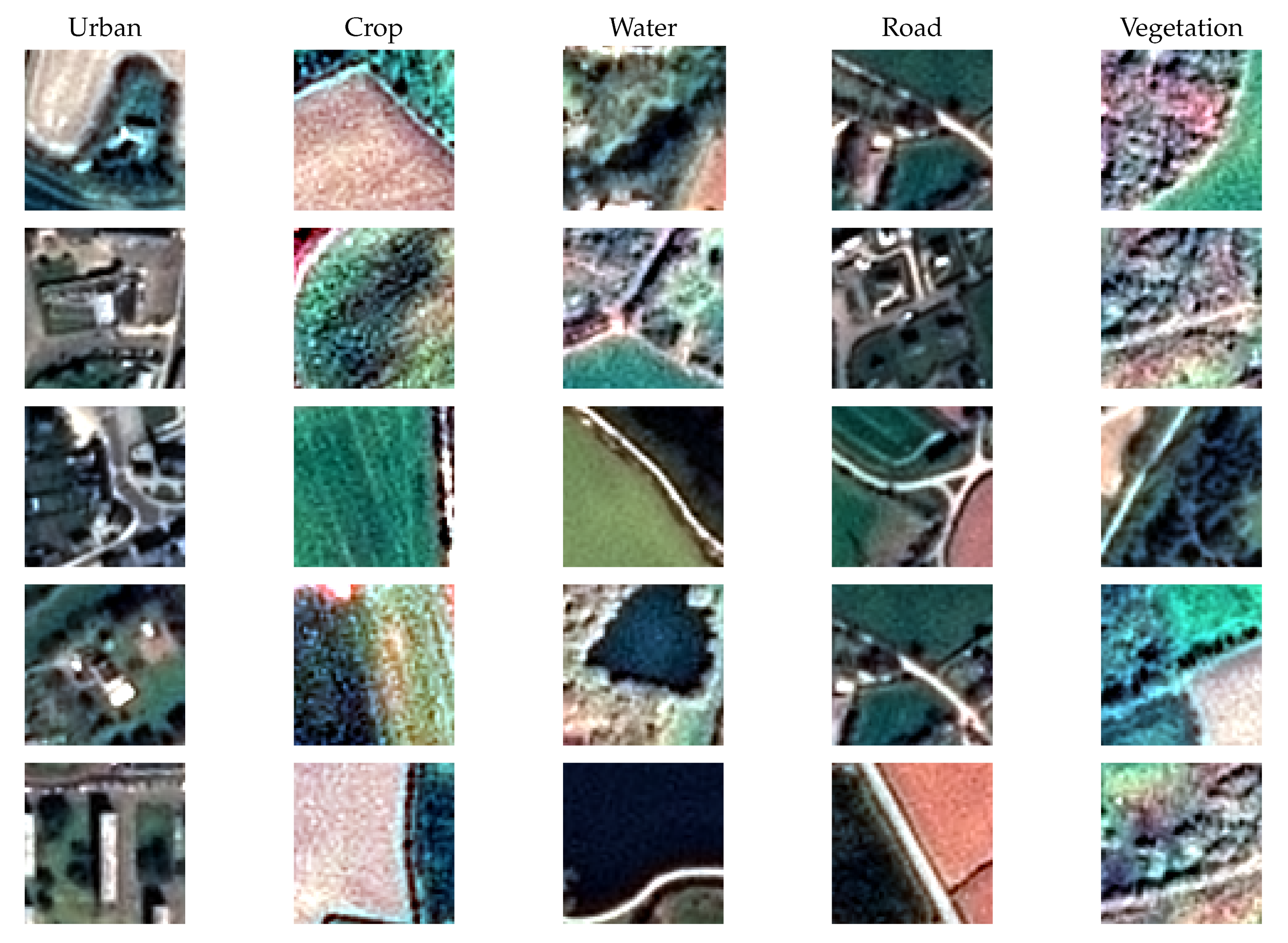
4.3. SPOT-7 Classification Problem

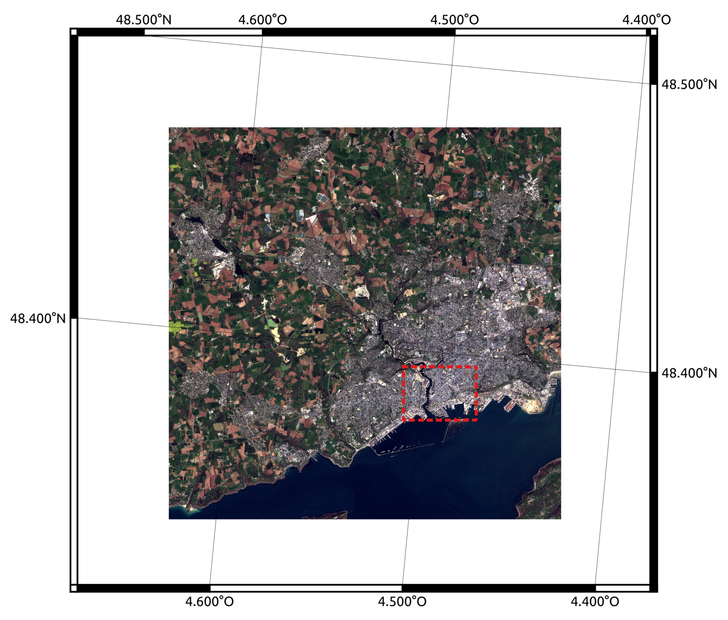
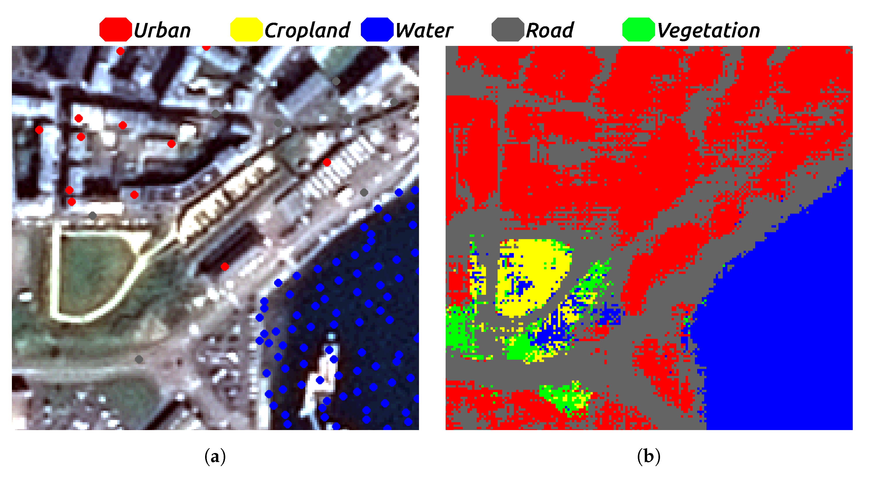
4.3.1. Description of the SPOT-7 Data Set

The second data set was based on optical imagery from SPOT-7, which measures surface reflectance in the visual RGB bands, as well as the Near Infrared band (NIR), at a spatial resolution of 6 m. Combined with a Panchromatic band at 1.50 m, a pan-sharpened RGB-NIR image could be obtained. The training data contains five classes: urban cover, roads, water, vegetation, and crops, which came from the BDTopo and Registre Parcellaire Graphique (RPG). This data set was identical to the one proposed in the experimental section of [50]. The challenging classes in this problem were the buildings (urban cover), the roads, and the water, due to common confusions between water and shade, which both appeared dark, and between the tones of gray that made up certain roofs and streets. In this situation, contextual information was key, as the shape, size, and texture of the objects was more relevant than the color of each individual pixel. Figure 14 provides an illustration of the full extent of the data set, which covers an area of 16.5 km × 16.5 km (11,000 × 11,000 pixels).

The aim of this set of experiments is to evaluate the validity of the HACCS method in a context with a lower number of pixel features than in the Sentinel-2 time series experiments. This is a way to study how applicable the HACCS method is to different types of data with unique temporal, spectral, and spatial characteristics.

This experimental setup compared four different initial classification results, and evaluates the application of HACCS on them. Indeed, the histograms of local classes could be calculated based on any previous dense classification of the image, which made HACCS applicable to any available result. The four methods are listed here.

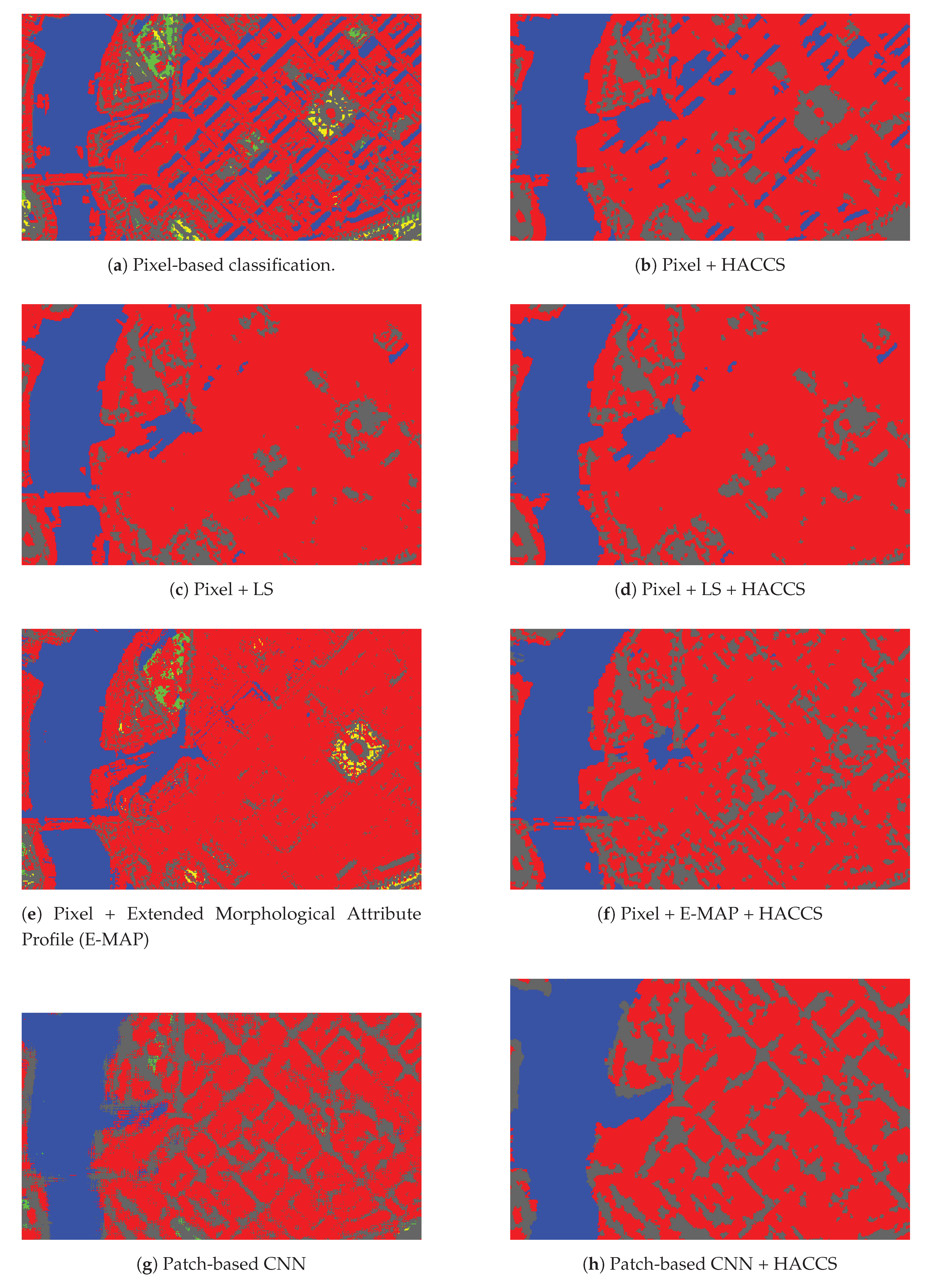
• The pixel-based classification. Applying HACCS here is the most basic scenario, and is essentially identical to what is done on the Sentinel-2 data set.
• The local statistic features, which in this scenario included the sample mean, variance, and edge density, defined in Section 2.1.
• The Extended Morphological Attribute Profiles (E-MAP), also defined in Section 2.1. These described context using several morphological operations on the image, with a structuring element of increasingly large size. Here, five structuring element sizes, ranging from 7 pixels to 15 pixels weare used to calculate E-MAP features using the brightness and Normalized Differential Vegetation Index (NDVI) over the area.
• The patch-based D-CNN designed by [50].

An illustration of different scales of superpixel segmentation that are calculated from the SPOT-7 image is given in Figure 15.

For training and validation of the supervised classification method, exactly 2000 training samples were randomly selected for each class. The Random Forest classifier was once again applied with a total of 100 trees.

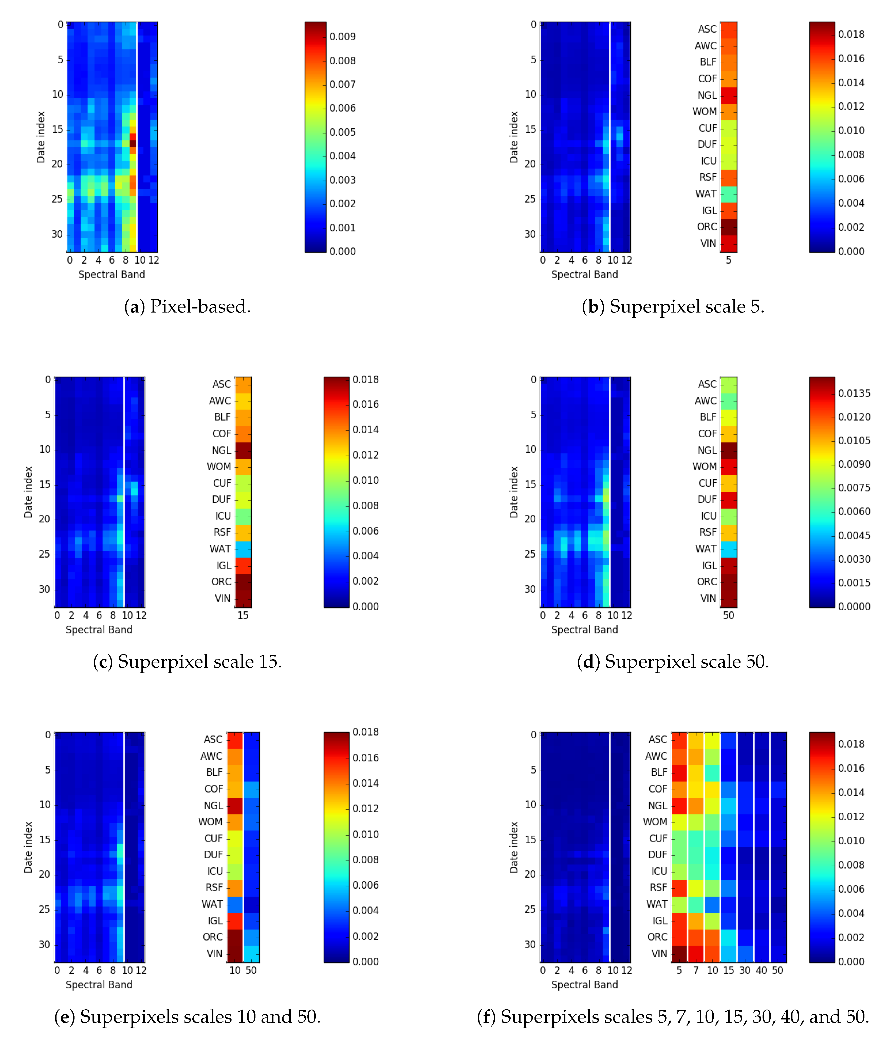
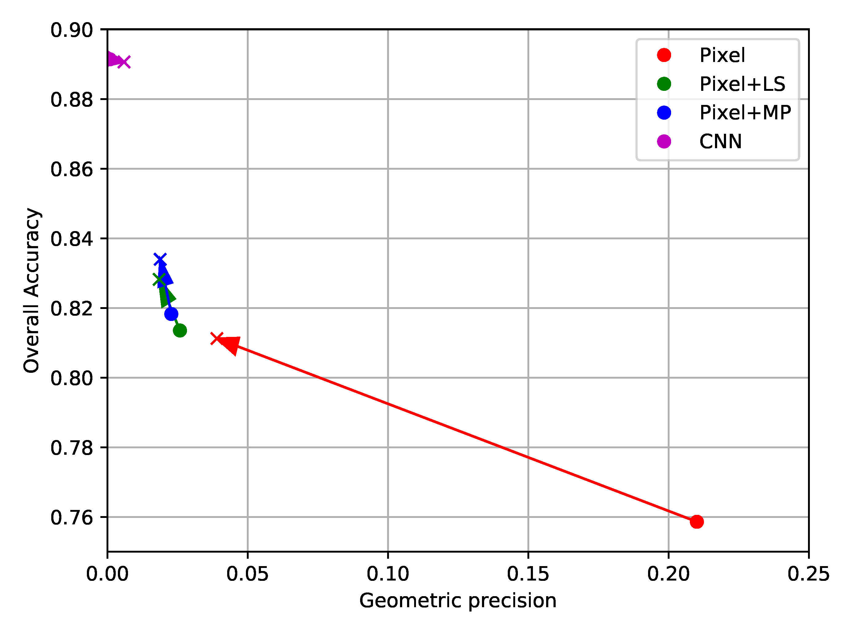
4.3.2. Results of the SPOT-7 Experiments

The experimental results are represented in three forms. First of all, Figure 16 shows the classification maps of the central area of the city of Brest. Next,

Table 6. Class accuracy (Overall Accuracy (OA), $\kappa$, and F-scores) and geometric accuracy (Pixel Based Corner Match (PBCM)) of the various methods on the SPOT-7 data set, expressed in percent units, along with the 1$\sigma$ error intervals. For the HACCS results, superpixel scales of 5, 10, 20, 30, 40, and 50 were used, with four iterations. In this table, LS stands for Local Statistics (mean, variance, and edge density), and E-MAP for Extended Morphological Attribute Profiles.

Method Name	OA (%)	Kappa (%)	PBCM (%)	Urban	Crop	Water	Road	Veg.
Pixel	75.86 ± 0.15	69.82 ± 0.19	21.01 ± 1.49	66.62	83.55	86.51	67.50	75.81
Pixel + HACCS	81.12 ± 0.16	76.40 ± 0.21	3.90 ± 0.55	74.96	88.00	91.48	69.35	81.86
Pixel + LS	81.35 ± 0.10	76.69 ± 0.12	2.58 ± 0.47	76.15	88.92	89.79	69.89	82.61
Pixel + LS + HACCS	82.82 ± 0.10	78.52 ± 0.12	1.84 ± 0.22	76.96	90.12	91.80	70.70	84.57
Pixel + E-MAP	81.82 ± 0.14	77.28 ± 0.18	2.28 ± 0.52	77.05	88.68	90.35	70.87	82.84
Pixel + E-MAP + HACCS	83.39 ± 0.10	79.24 ± 0.13	1.88 ± 0.18	78.21	90.01	91.75	72.22	84.98
CNN	89.13 ± 0.06	86.42 ± 0.07	0.09 ± 0.04	86.22	93.20	96.13	81.32	88.59
CNN + HACCS	89.06 ± 0.09	86.32 ± 0.11	0.59 ± 0.08	85.74	93.62	95.89	80.80	89.07

provides the numerical values of the classification accuracy scores: OA, Kappa, as well as the F-scores of the different methods. Finally, Figure 17 compares the semantic and geometrical accuracy of the various methods by plotting the OA against the PBCM.

Figure 16a shows the result of a pixel-based Random Forest on the central urban area, which illustrates the importance of contextual information in this problem. Indeed, with only the pixel information available, there were several confusions between the contextual classes mentioned earlier: urban cover, roads, and water.

In Figure 16b, the multi-scale class histogram features are directly calculated from the pixel based classification, as is done on the high-dimensional Sentinel-2 time series. The HACCS process allowed for a better discrimination between the context dependent classes mentioned above. Indeed, the presence of water and vegetation classes in the urban area was somewhat reduced when compared to the pixel-based classification. However, this result is not entirely satisfactory, as many confusions remained, especially between roads and buildings in the city center. It is worth mentioning that in all of the experimental results presented here, the class histogram features were calculated in superpixels at scales 5, 10, 20, 30, 40, and 50. In preliminary experiments, this has shown to provide more precise results than using only one scale at a time. Figure 16b shows that the HACCS process allowed for a better discrimination between the context-dependent classes in the urban area. Indeed, the presence of water and vegetation classes in the urban area was somewhat reduced when compared to the pixel-based classification, although this result is not entirely satisfactory, as many confusions remained, especially between roads and buildings in the city center.

The classification result in Figure 16c was generated using standard local statistics: sample mean, variance, and edge density [67]. These image based contextual features were calculated in the same spatial supports as the class histograms. The result of this classification is shown in Figure 16c. While the use of local statistics allowed for the confusions between roads and water to be greatly diminished, there still remained confusions between roads and urban cover. This is certainly progress, but it would be desirable to observe the details of the network of roads and streets in the classification result. The impact of applying the HACCS process to this result is shown in Figure 16d. In this case, the HACCS process provided a smoother result, although many confusions remained between roads, buildings, and water.

Figure 16e shows the classified urban area, based on both the pixel and the E-MAP features. Figure 16f shows the obtained classification map when using the histogram of the classes from the pixel and E-MAP feature result. In this image, many of the streets were recognized, and the fine geometrical elements, such as the harbor and the bridges were correctly restored. However, the streets that were recognized were disconnected and spread out through the urban area. This would not be sufficient for determining the precise network of streets.

Finally, HACCS was also applied to the result of the CNN. This was done to evaluate whether or not HACCS could improve the quality of a classification that was already very accurate. It appears that the result after HACCS did not restore much of the high spatial frequency geometry, such as the fine details of the harbor. On the other hand, it had a smoothing effect everywhere in the image, which removed isolated pixels and other kinds of label pixel noise. Moreover, the borders between objects had a relatively clear definition, with some of the corners being restored.

Table 6 shows that including contextual information improves the F-score of all of the classes compared to the pixel-based classification, for all of the methods that were evaluated here. Secondly, it can be noted that the HACCS iterations never made the F-score values decrease, except for when initialized on the CNN result, where a slight decrease was observed for three of the five classes.

The best performing method overall was the CNN, which was relatively equivalent in terms of overall performance scores to the CNN + HACCS, although the latter had a slightly higher PBCM. In second place, the E-MAP features, particularly combined with HACCS, provided an improvement over the pixel-based classification (≈+7.5% in OA), reaching approximately half of the improvement achieved by the CNN (≈+15% in OA).

It should be noted that the low values of PBCM can be attributed to the noise present in the pixel-based classification which makes corners more difficult to detect, regardless of the calibration parameters of the line detector. This effect may be due to the application of this metric to very high spatial resolution imagery, in which the pixel-based classification is more subject to such errors than in high resolution imagery.

Finally, Figure 17 shows how the geometric precision, as measured by the PBCM, evolves with the overall accuracy when applying the HACCS process. The solid point at the root of the arrow shows the scores of the initial classification, the iteration 0 of the HACCS process, which was used for the first estimation of the histograms. The head of the arrow is positioned according to the scores after four iterations of the HACCS process, with a cross at the convergence point. For the pixel, local statistics, and E-MAP features, applying the HACCS iterative process improves the overall accuracy, while diminishing or maintaining the geometric precision of the result. On the other hand, applying iterations of HACCS on the result from the patch-based CNN slightly decreases the overall accuracy, but restores some of the sharp corners, which are measured by the PBCM.

Overall, the application of this network to SPOT-7 strongly increases the classification accuracies of the context-dependent classes. However, the level of detail around the edges of the objects is very often blurry, and presents a number of noisy decisions, particularly around the class boundaries. This is illustrated in Figure 18b, which shows the classification result of the D-CNN on an urban area.

This may be explained by the fact that the training data that were used for this classification presented a strong concentration of training pixels in the center of the objects, which means that an extensive description of the class boundaries is missing. This is representative of a land cover mapping problem over wide areas, in which the only available training data sets are sparsely labeled. This example shows how a bias in the training data can cause visible errors in the result, in areas that are entirely absent from the training data. These results suggest that methods that rely solely on the training data to learn every single aspect of a classification problem can be subject to generalization errors, if the training data are not sufficiently representative of the problem.

5. Discussion

The first classification problem, presented in Section 4.2, is a land cover mapping problem over 110 × 110 tiles covering parts of the French territory. The use of 10 m spatial resolution Sentinel-2 time series enables a variety of natural, agricultural, and artificial classes to be recognized using supervised classification methods. Training data for these methods almost always come in a sparse form, which is why this case study is representative of a real world land cover mapping problem. Moreover, high-dimensional time series are rarely used in combination with contextual features, due to limitations in the total number of features that can be simultaneously considered by a supervised classifier. The main advantage of the HACCS process is that it does not require very many features. Indeed, the number of features is conditioned by the class nomenclature and the number of scales, and not by the type of imagery, making it adapted for classifying images presenting a great number of original pixel features. The experiments on this data set show that the HACCS process provides a similar performance to the CNN architecture in terms of overall accuracy. Moreover, the HACCS process produces maps with a higher geometric accuracy, measured by how well the classification can restore sharp corners compared to a pixel-based classification. This result is consistent across 11 Sentinel-2 tiles, which each cover an area of around ten thousand square kilometers, meaning that the proposed method is relatively robust to differences in class proportion and land cover class behavior.

Next, the same methods are applied to imagery from SPOT-7. Unlike the Sentinel-2 time series, these images are mono-date, have a far finer spatial resolution of 1.5 m, and have a lower spectral resolution with only three visible bands and one infrared band. This implies that each pixel originally contains a relatively low number of features, however, more pixels are required to cover an equivalent zone. Two groups of standard contextual features are evaluated on this problem: the Local Statistics (LS), which contain sample mean, variance, and edge density, and Extended Morphological Attribute Profiles (E-MAP). Alone, the E-MAP features provide both the highest values of OA, with similar values of PBCM as the LS features.

Then, experiments are run where the histograms are based on a classification result that is already generated with contextual features. Using several iterations of HACCS in multiple superpixel scales allows for a consistent improvement of the precision of each class. However, some of the corners present in the pixel-based classification are displaced or lost. When comparing these results to the classification map generated by the patch-based CNN from [50], it appears that the handcrafted features (LS, E-MAP, HACCS), provide lower values of overall accuracy on this problem. Indeed, very high spatial resolution problems with a low number of image features are similar to the Computer Vision problems for which these networks were originally designed. On the other hand, the handcrafted features generally show a higher degree of geometric precision, in other words, they contain well localized sharp corners. This is both visible in the classification maps, and quantified by the experiments run on this data set.

The results presented in Section 4.3 show that the HACCS process generates a pertinent contextual description, even for low-dimensional images at a higher spatial resolution. Alone, HACCS provides comparable results to other contextual features like local statistics and Extended Morphological Profiles. When combining the HACCS process with the standard contextual features, the classification accuracy after a few iterations is significantly improved. However, on this type of mono-date high spatial resolution imagery, the patch-based CNN does provide an overall more accurate classification result.

It can be noted that using a patch-based image classification network for semantic labeling, as was done in the SPOT experiments, is far from ideal, seeing as this is not the original purpose of these networks. However, we believe that there are other important aspects to this issue. Firstly, these patch-based networks have no requirement on the density of the labeled data: they can be trained even on data sets containing only labeled pixels spread very sparsely in the image, which does make them interesting candidates for such extreme cases. Secondly, it remains interesting to observe the results of such networks when applied to a semantic labeling problem. In fact, the SPOT experiments show that these networks do not totally fail, as one might expect. They have very strong detection capabilities, and are able to detect roads where methods using contextual features with adaptive neighborhoods are unable to. Their main issue seems to be in precisely localizing the edges of objects. Thirdly, there have been experiments on very high spatial resolution imagery (Pl∖’eiades) which have shown that even fully-convolutional architectures such as Unet also have issues in providing results with an accurate geometry, particularly when faced with noisy training data sets, and that this effect is reduced when fine-tuning the network with manually corrected data [6].

6. Conclusions and Perspectives

In this paper, the Histogram of Auto-Context Classes in Superpixels (HACCS) process is evaluated as a new method for generating land cover maps with context-dependent classes, in the absence of dense training data. The contextual feature that is used is the histogram of class predictions, in one or more superpixels [46,47] of different sizes. These predictions can either be taken from a pixel-based classification or a classification with contextual features, which allows the method to operate starting with any classification result, and iterated several times, as is shown in Figure 1.

This method is compared to the current state-of-the-art methods for including contextual information in dense classification schemes, Convolutional Neural Networks. The architecture of these networks is designed to take a patch of pixels as an input, which allows for an end-to-end optimization of both the feature extraction and feature selection steps.

Overall, in these two very different land cover classification experiments, the use of Convolutional Neural Networks seems to provide lower degrees of geometric accuracy than superpixel based methods with handcrafted features. This may be due to the sparsity of the training data, which are insufficient to describe the geometry of the objects during training. In other words, the neural network is not discouraged for generating results with smooth corners, as these corners are absent from the training data, and therefore from the loss function. On the other hand, superpixel-based methods extract the geometry of the objects directly from the image, which in many cases preserves the geometry. This conclusion must be taken with care as it is based partly on a visual validation and therefore is limited to the area that was analysed in detail.

Secondly, in high-dimensional feature spaces, such as the time series used in the Sentinel-2 experiment, it appears the HACCS process provides results with equivalent levels of class accuracy as the FG-Unet architecture [53]. Moreover, the HACCS results systematically present a higher rate of geometric accuracy, with a finer localization of sharp corners. It also is worth mentioning that the HACCS process is computationally lighter than neural networks, as it only involves the training of a Random Forest for each iteration, which is very fast in practice. It would be interesting to study whether these results can be extended to hyperspectral images that also present a very high number of image features.

Finally, when using images with similar characteristics to the ones encountered in Computer Vision problems, i.e., a very high spatial resolution, and a low number of features per pixel, the CNNs show the strongest levels of class accuracy. On the other hand, the geometry of the result is questionable, with the presence of speckle-like label noise near object boundaries, and smooth corners. Handcrafted features in superpixels, like HACCS, allow for higher levels of geometric precision. In further studies, it would be interesting to evaluate the effect of the density of training data on the geometry of the classification map, and the application of HACCS to other dense image classification problems, such as hyperspectral or radar imagery.

Overall, this study suggests that for the higher spatial resolution images with fewer features (SPOT-7) the use of CNNs may be preferred, under the condition that a higher computational cost and lower geometric accuracy is acceptable. Moreover, if HACCS is applied to such images it must be done with care, as if the number of contextual features largely exceeds the number of pixel features, it may result in a degradation of the geometry. For HSR imagery (Sentinel-2) with more pixel features, HACCS seems to be the preferred solution, seeing as it provides a similar performance with a lower computational cost.

The source code for the HACCS process is based on the use of the open source software Orfeo ToolBox, and is freely available [68].

References

1. Petitjean, F.; Inglada, J.; Gançarski, P. Satellite image time series analysis under time warping. IEEE Trans. Geosci. Remote Sens. 2012, 50, 3081–3095. [Google Scholar] [CrossRef]
2. Gómez, C.; White, J.C.; Wulder, M.A. Optical remotely sensed time series data for land cover classification: A review. ISPRS J. Photogramm. Remote Sens. 2016, 116, 55–72. [Google Scholar] [CrossRef] [Green Version]
3. Thanh Noi, P.; Kappas, M. Comparison of random forest, k-nearest neighbor, and support vector machine classifiers for land cover classification using Sentinel-2 imagery. Sensors 2018, 18, 18. [Google Scholar] [CrossRef] [PubMed] [Green Version]
4. Griffiths, P.; Nendel, C.; Hostert, P. Intra-annual reflectance composites from Sentinel-2 and Landsat for national-scale crop and land cover mapping. Remote Sens. Environ. 2019, 220, 135–151. [Google Scholar] [CrossRef]
5. Inglada, J.; Vincent, A.; Arias, M.; Tardy, B.; Morin, D.; Rodes, I. Operational high resolution land cover map production at the country scale using satellite image time series. Remote Sens. 2017, 9, 95. [Google Scholar] [CrossRef] [Green Version]
6. Maggiori, E.; Tarabalka, Y.; Charpiat, G.; Alliez, P. Convolutional neural networks for large-scale remote-sensing image classification. IEEE Trans. Geosci. Remote Sens. 2017, 55, 645–657. [Google Scholar] [CrossRef] [Green Version]
7. Hinton, G.E.; Srivastava, N.; Krizhevsky, A.; Sutskever, I.; Salakhutdinov, R.R. Improving neural networks by preventing co-adaptation of feature detectors. arXiv 2012, arXiv:1207.0580. [Google Scholar]
8. Simard, P.Y.; Steinkraus, D.; Platt, J.C. Best practices for convolutional neural networks applied to visual document analysis. Icdar IEEE 2003, 3, 958. [Google Scholar]
9. Chellapilla, K.; Shilman, M.; Simard, P. Optimally combining a cascade of classifiers. In Proceedings of the Recognition and Retrieval XIII International Society for Optics and Photonics, San Jose, CA, USA, 16 January 2006; Volume 6067, p. 60670Q. [Google Scholar]
10. Chellapilla, K.; Puri, S.; Simard, P. High performance convolutional neural networks for document processing. In Proceedings of the Tenth International Workshop on Frontiers in Handwriting Recognition, Suvisoft, La Baule, France, 23–26 October 2006. [Google Scholar]
11. Krizhevsky, A.; Sutskever, I.; Hinton, G.E. Imagenet classification with deep convolutional neural networks. In Proceedings of the Advances in Neural Information Processing Systems, Lake Tahoe, NV, USA, 3–6 December 2012; pp. 1097–1105. [Google Scholar]
12. Marmanis, D.; Schindler, K.; Wegner, J.D.; Galliani, S.; Datcu, M.; Stilla, U. Classification with an edge: Improving semantic image segmentation with boundary detection. ISPRS J. Photogramm. Remote Sens. 2018, 135, 158–172. [Google Scholar] [CrossRef] [Green Version]
13. Xie, S.; Tu, Z. Holistically-nested edge detection. In Proceedings of the IEEE International Conference on Computer Vision, Santiago, Chile, 7–13 December 2015; pp. 1395–1403. [Google Scholar]
14. Drucker, H.; Burges, C.J.; Kaufman, L.; Smola, A.J.; Vapnik, V. Support vector regression machines. In Advances in Neural Information Processing Systems; MIT Press: Cambridge, MA, USA, 1997; pp. 155–161. [Google Scholar]
15. Breiman, L. Random forests. Mach. Learn. 2001, 45, 5–32. [Google Scholar] [CrossRef] [Green Version]
16. Haralick, R.M. Statistical and structural approaches to texture. Proc. IEEE 1979, 67, 786–804. [Google Scholar] [CrossRef]
17. Coburn, C.; Roberts, A.C. A multiscale texture analysis procedure for improved forest stand classification. Int. J. Remote Sens. 2004, 25, 4287–4308. [Google Scholar] [CrossRef] [Green Version]
18. Yu, Q.; Gong, P.; Clinton, N.; Biging, G.; Kelly, M.; Schirokauer, D. Object-based detailed vegetation classification with airborne high spatial resolution remote sensing imagery. Photogramm. Eng. Remote Sens. 2006, 72, 799–811. [Google Scholar] [CrossRef] [Green Version]
19. Blaschke, T. Object based image analysis for remote sensing. ISPRS J. Photogramm. Remote Sens. 2010, 65, 2–16. [Google Scholar] [CrossRef] [Green Version]
20. Walker, J.; Blaschke, T. Object-based land-cover classification for the Phoenix metropolitan area: Optimization vs. transportability. Int. J. Remote Sens. 2008, 29, 2021–2040. [Google Scholar] [CrossRef]
21. D’Oleire Oltmanns, S.; Marzolff, I.; Tiede, D.; Blaschke, T. Detection of gully-affected areas by applying object-based image analysis (OBIA) in the region of Taroudannt, Morocco. Remote Sens. 2014, 6, 8287–8309. [Google Scholar] [CrossRef] [Green Version]
22. Lowe, D.G. Object recognition from local scale-invariant features. In Proceedings of the Seventh IEEE International Conference on IEEE, Computer Vision, Kerkyra, Greece, 20–27 September 1999; Volume 2, pp. 1150–1157. [Google Scholar]
23. Bay, H.; Tuytelaars, T.; Van Gool, L. Surf: Speeded up robust features. In Proceedings of the European Conference on Computer Vision, Graz, Austria, 7–13 May 2006; Springer: Berlin, Germany, 2006; pp. 404–417. [Google Scholar]
24. Pham, M.T.; Mercier, G.; Michel, J. PW-COG: An effective texture descriptor for VHR satellite imagery using a pointwise approach on covariance matrix of oriented gradients. IEEE Trans. Geosci. Remote Sens. 2016, 54, 3345–3359. [Google Scholar] [CrossRef]
25. Benediktsson, J.A.; Palmason, J.A.; Sveinsson, J.R. Classification of hyperspectral data from urban areas based on extended morphological profiles. IEEE Trans. Geosci. Remote Sens. 2005, 43, 480–491. [Google Scholar] [CrossRef]
26. Fauvel, M.; Benediktsson, J.A.; Chanussot, J.; Sveinsson, J.R. Spectral and spatial classification of hyperspectral data using SVMs and morphological profiles. IEEE Trans. Geosci. Remote Sens. 2008, 46, 3804–3814. [Google Scholar] [CrossRef] [Green Version]
27. Dalla Mura, M.; Villa, A.; Benediktsson, J.A.; Chanussot, J.; Bruzzone, L. Classification of hyperspectral images by using extended morphological attribute profiles and independent component analysis. IEEE Geosci. Remote Sens. Lett. 2010, 8, 542–546. [Google Scholar] [CrossRef] [Green Version]
28. Song, B.; Li, J.; Dalla Mura, M.; Li, P.; Plaza, A.; Bioucas-Dias, J.M.; Benediktsson, J.A.; Chanussot, J. Remotely sensed image classification using sparse representations of morphological attribute profiles. IEEE Trans. Geosci. Remote Sens. 2014, 52, 5122–5136. [Google Scholar] [CrossRef] [Green Version]
29. Yang, Y.; Newsam, S. Bag-of-visual-words and spatial extensions for land-use classification. In Proceedings of the 18th SIGSPATIAL International Conference on Advances in Geographic Information Systems, San Jose, CA, USA, 2–5 November 2010; pp. 270–279. [Google Scholar]
30. Russell, B.C.; Freeman, W.T.; Efros, A.A.; Sivic, J.; Zisserman, A. Using multiple segmentations to discover objects and their extent in image collections. In Proceedings of the 2006 Conference on IEEE Computer Society Computer Vision and Pattern Recognition, New York, NY, USA, 17–22 June 2006; Volume 2, pp. 1605–1614. [Google Scholar]
31. Larios, N.; Lin, J.; Zhang, M.; Lytle, D.; Moldenke, A.; Shapiro, L.; Dietterich, T. Stacked spatial-pyramid kernel: An object-class recognition method to combine scores from random trees. In Proceedings of the 2011 IEEE Workshop on Applications of Computer Vision (WACV), Kona, HI, USA, 5–7 January 2011; pp. 329–335. [Google Scholar]
32. Moser, G.; Serpico, S.B. Combining support vector machines and Markov random fields in an integrated framework for contextual image classification. IEEE Trans. Geosci. Remote Sens. 2013, 51, 2734–2752. [Google Scholar] [CrossRef]
33. Zhao, J.; Zhong, Y.; Shu, H.; Zhang, L. High-Resolution Image Classification Integrating Spectral-Spatial- Location Cues by Conditional Random Fields. IEEE Trans. Image Process. 2016, 25, 4033–4045. [Google Scholar] [CrossRef] [PubMed]
34. Shotton, J.; Johnson, M.; Cipolla, R. Semantic texton forests for image categorization and segmentation. In Proceedings of the 2008 IEEE Conference on Computer Vision and Pattern Recognition, Anchorage, AK, USA, 23–28 June 2008; pp. 1–8. [Google Scholar]
35. Fröhlich, B.; Rodner, E.; Denzler, J. Semantic segmentation with millions of features: Integrating multiple cues in a combined random forest approach. In Asian Conference on Computer Vision; Springer: Berlin, Germany, 2012; pp. 218–231. [Google Scholar]
36. Tu, Z. Auto-context and its application to high-level vision tasks. In Proceedings of the IEEE Conference on Computer Vision and Pattern Recognition, CVPR 2008, Anchorage, AK, USA, 23–28 June 2008; pp. 1–8. [Google Scholar]
37. Tu, Z.; Bai, X. Auto-context and its application to high-level vision tasks and 3d brain image segmentation. IEEE Trans. Pattern Anal. Mach. Intell. 2010, 32, 1744–1757. [Google Scholar] [PubMed]
38. Jiang, J.; Tu, Z. Efficient scale space auto-context for image segmentation and labeling. In Proceedings of the IEEE Conference on Computer Vision and Pattern Recognition, CVPR 2009, Miami, FL, USA, 20–25 June 2009; pp. 1810–1817. [Google Scholar]
39. Fröhlich, B.; Bach, E.; Walde, I.; Hese, S.; Schmullius, C.; Denzler, J. Land cover classification of satellite images using contextual information. ISPRS Ann. Photogramm. Remote Sens. Spat. Inf. Sci. 2013, 3, W1. [Google Scholar] [CrossRef] [Green Version]
40. Jampani, V.; Gadde, R.; Gehler, P.V. Efficient facade segmentation using auto-context. In Proceedings of the 2015 IEEE Winter Conference on Applications of Computer Vision (WACV), Waikoloa, HI, USA, 5–9 January 2015; pp. 1038–1045. [Google Scholar]
41. Huynh, T.; Gao, Y.; Kang, J.; Wang, L.; Zhang, P.; Lian, J.; Shen, D. Estimating CT image from MRI data using structured random forest and auto-context model. IEEE Trans. Med. Imaging 2016, 35, 174. [Google Scholar] [CrossRef] [PubMed] [Green Version]
42. Munoz, D.; Bagnell, J.A.; Hebert, M. Stacked hierarchical labeling. In European Conference on Computer Vision; Springer: Berlin, Germany, 2010; pp. 57–70. [Google Scholar]
43. Derksen, D.; Inglada, J.; Michel, J. A Metric for Evaluating the Geometric Quality of Land Cover Maps Generated with Contextual Features from High-Dimensional Satellite Image Time Series without Dense Reference Data. Remote Sens. 2019, 11, 1929. [Google Scholar] [CrossRef] [Green Version]
44. Comaniciu, D.; Meer, P. Mean shift: A robust approach toward feature space analysis. IEEE Trans. Pattern Anal. Mach. Intell. 2002, 24, 603–619. [Google Scholar] [CrossRef] [Green Version]
45. Baatz, M. Multiresolution segmentation: An optimization approach for high quality multi-scale image segmentation. In Proceedings of the Angewandte Geographische Informationsverarbeitung, Salzburg, Germany, 5–7 June 2000; pp. 12–23. [Google Scholar]
46. Achanta, R.; Shaji, A.; Smith, K.; Lucchi, A.; Fua, P.; Süsstrunk, S. SLIC superpixels compared to state-of-the-art superpixel methods. IEEE Trans. Pattern Anal. Mach. Intell. 2012, 34, 2274–2282. [Google Scholar] [CrossRef] [Green Version]
47. Derksen, D.; Inglada, J.; Michel, J. Scaling Up SLIC Superpixels Using a Tile-Based Approach. IEEE Trans. Geosci. Remote Sens. 2019, 1–13. [Google Scholar] [CrossRef]
48. Penatti, O.A.; Nogueira, K.; dos Santos, J.A. Do deep features generalize from everyday objects to remote sensing and aerial scenes domains? In Proceedings of the IEEE Conference on Computer Vision and Pattern Recognition Workshops, Boston, MA, USA, 7–12 June 2015; pp. 44–51. [Google Scholar]
49. Marmanis, D.; Datcu, M.; Esch, T.; Stilla, U. Deep learning earth observation classification using ImageNet pretrained networks. IEEE Geosci. Remote Sens. Lett. 2016, 13, 105–109. [Google Scholar] [CrossRef] [Green Version]
50. Postadjian, T.; Le Bris, A.; Sahbi, H.; Mallet, C. Investigating the Potential of Deep Neural Networks for Large-Scale Classification of Very High Resolution Satellite Images. ISPRS Ann. Photogramm. Remote Sens. Spat. Inf. Sci. 2017, 183–190. [Google Scholar] [CrossRef] [Green Version]
51. Badrinarayanan, V.; Kendall, A.; Cipolla, R. Segnet: A deep convolutional encoder-decoder architecture for image segmentation. arXiv 2015, arXiv:1511.00561. [Google Scholar] [CrossRef]
52. Ronneberger, O.; Fischer, P.; Brox, T. U-net: Convolutional networks for biomedical image segmentation. In Proceedings of the International Conference on Medical Image Computing and Computer-Assisted Intervention, Munich, Germany, 5–9 October 2015; Springer: Berlin, Germany, 2015; pp. 234–241. [Google Scholar]
53. Stoian, A.; Poulain, V.; Inglada, J.; Poughon, V.; Derksen, D. Land Cover Maps Production with High Resolution Satellite Image Time Series and Convolutional Neural Networks: Adaptations and Limits for Operational Systems. Remote Sens. 2019, 11, 1986. [Google Scholar] [CrossRef] [Green Version]
54. Kussul, N.; Lavreniuk, M.; Skakun, S.; Shelestov, A. Deep learning classification of land cover and crop types using remote sensing data. IEEE Geosci. Remote Sens. Lett. 2017, 14, 778–782. [Google Scholar] [CrossRef]
55. Chen, Y.; Lin, Z.; Zhao, X.; Wang, G.; Gu, Y. Deep learning-based classification of hyperspectral data. IEEE J. Sel. Top. Appl. Earth Obs. Remote Sens. 2014, 7, 2094–2107. [Google Scholar] [CrossRef]
56. Kampffmeyer, M.; Salberg, A.B.; Jenssen, R. Semantic segmentation of small objects and modeling of uncertainty in urban remote sensing images using deep convolutional neural networks. In Proceedings of the IEEE Conference on Computer Vision and Pattern Recognition Workshops, Las Vegas, NV, USA, 26 June–1 July 2016; pp. 1–9. [Google Scholar]
57. Audebert, N.; Le Saux, B.; Lefèvre, S. Semantic segmentation of earth observation data using multimodal and multi-scale deep networks. In Asian Conference on Computer Vision; Springer: Berlin, Germany, 2016; pp. 180–196. [Google Scholar]
58. Hoover, A.; Jean-Baptiste, G.; Jiang, X.; Flynn, P.J.; Bunke, H.; Goldgof, D.B.; Bowyer, K.; Eggert, D.W.; Fitzgibbon, A.; Fisher, R.B. An experimental comparison of range image segmentation algorithms. IEEE Trans. Pattern Anal. Mach. Intell. 1996, 18, 673–689. [Google Scholar] [CrossRef] [Green Version]
59. Everingham, M.; Van Gool, L.; Williams, C.K.; Winn, J.; Zisserman, A. The Pascal Visual Object Classes (VOC) Challenge. Int. J. Comput. Vis. 2010, 88, 303–338. [Google Scholar] [CrossRef] [Green Version]
60. Bruzzone, L.; Carlin, L. A multilevel context-based system for classification of very high spatial resolution images. IEEE Trans. Geosci. Remote Sens. 2006, 44, 2587–2600. [Google Scholar] [CrossRef] [Green Version]
61. Huang, X.; Zhang, L.; Li, P. A multiscale feature fusion approach for classification of very high resolution satellite imagery based on wavelet transform. Int. J. Remote Sens. 2008, 29, 5923–5941. [Google Scholar] [CrossRef]
62. Bossard, M.; Feranec, J.; Otahel, J. CORINE Land Cover Technical Guide: Addendum 2000; European Environment Agency: Copenhagen, Denmark, 2000. [Google Scholar]
63. Montero, E.; Van Wolvelaer, J.; Garzón, A. The European urban atlas. In Land Use and Land Cover Mapping in Europe; Springer: Berlin, Germany, 2014; pp. 115–124. [Google Scholar]
64. Maugeais, E.; Lecordix, F.; Halbecq, X.; Braun, A. Dérivation cartographique multi échelles de la BDTopo de l’IGN France: Mise en œuvre du processus de production de la Nouvelle Carte de Base. In Proceedings of the 25th International Cartographic Conference, Paris, France, 3–8 July 2011; pp. 3–8. [Google Scholar]
65. Cantelaube, P.; Carles, M. Le registre parcellaire graphique: Des données géographiques pour décrire la couverture du sol agricole. In Le Cahier des Techniques de l’INRA; 2014; pp. 58–64. Available online: https://www6.inrae.fr/cahier_des_techniques/content/download/3813/34098/version/2/file/12_CH2_CANTELAUBE_registre_parcellaire.pdf (accessed on 2 February 2020).
66. Pfeffer, W.T.; Arendt, A.A.; Bliss, A.; Bolch, T.; Cogley, J.G.; Gardner, A.S.; Hagen, J.O.; Hock, R.; Kaser, G.; Kienholz, C.; et al. The Randolph Glacier Inventory: A globally complete inventory of glaciers. J. Glaciol. 2014, 60, 537–552. [Google Scholar] [CrossRef] [Green Version]
67. Trias Sanz, R. Semi-Automatic Rural Land Cover Classification. Ph.D. Thesis, Université Paris 5, Paris, France, 2006. [Google Scholar]
68. Derksen, D. Source Code of Histogram of Auto-Context Classes. 2019. Available online: https://github.com/derksend/histogram-auto-context (accessed on 9 August 2019).
Figure 1. The Histogram of Auto-Context Classes in Superpixels process. A dense labeling of all the pixels is used to compute the histogram of the different classes. This histogram provides a contextual characterization, which serves as a supplementary feature for the next classification step, to refine the decision based on nearby contextual cues. The initial dense prediction can also originate from a different classification system, such as a Convolutional Neural Network (CNN).
Remotesensing 12 00513 g001
Figure 2. Superpixel and Mean-shift segmentations of a Sentinel-2 image time series, on a discontinuous urban fabric area. Background: RGB bands of the first date. The segmentation was applied using all of the dates and all of the spectral bands simultaneously. (a) SLIC superpixels. Superpixels contain spectraly diverse pixels, which allows to describe textured areas. Homogeneous areas are undersegmented, but contain a sufficient amount of pixels for a proper description; (b) Mean-shift segmentation. The urban area is oversegmented, due to the high spectral variability, meaning that the segments are unable to describe the texture.
Remotesensing 12 00513 g002
Figure 3. Architecture of the patch-based network that is used for comparison with the Histogram of Auto Context Classes in Superpixels (HACCS), identical to the work in [50]. The first layer intakes a neighborhood of 65 × 65 pixels around the central pixel. Then, this relatively shallow network contains three stages of convolution and max-pooling, followed by a fully connected layer.
Remotesensing 12 00513 g003
Figure 4. Images of labeled patches used by the patch-based Convolutional Neural Network.
Remotesensing 12 00513 g004
Figure 5. Fully convolutional architecture used on the Sentinel-2 data set in [53]. Inspired by the U-Net architecture, it contains several convolution and max-pooling stages, followed by deconvolution and unpooling, to generate a dense prediction of the patch. A 3-date weight sharing scheme, as well as a 1 × 1 convolution stage were used to adapt this problem to use with time series, and sparsely labeled data.
Remotesensing 12 00513 g005
Figure 6. Sparsely labeled training samples over the city of Saint-Nazaire. Background: RGB bands of the first date of the time series (January 2016).
Remotesensing 12 00513 g006
Figure 7. Extent and naming convention of the 11 Sentinel-2 tiles. These tiles cover a variety of landscapes, with very different climatic conditions and thematic content.
Remotesensing 12 00513 g007
Figure 8. Image of the first date of the Sentinel-2 time series over the T30TWT tile in Brittany. The red dotted rectangle shows the location of the city of Saint-Nazaire, which is the focus of Figure 9 and Figure 11. The cloud detection and removal, which are detailed in [5], are not perfect at each individual date, but the overall time series still provides very useful information for classifying land cover.
Remotesensing 12 00513 g008
Figure 9. Evolution of the multi-scale HACCS classification result throughout three iterations. At each iteration, the result of the previous classification is used to re-estimate the histograms in several scales of superpixels, which are used as contextual features. Most of the differences are observed at iteration 1, when contextual information is included for the first time. After a few iterations, the classification result shows very few changes between successive iterations.
Remotesensing 12 00513 g009
Figure 10. Iterations of the HACCS process. The arrows represent successive iterations, which start from the pixel-based classification, and reach the convergence point once no significant change is detected. The numbers and colors represent the different tiles, once again following the definitions from Table 2.
Remotesensing 12 00513 g010
Figure 11. Results of the classification of the three methods over an urban area (Saint-Nazaire, see Figure 8) in the T30TWT tile. The pixel based result contains a strong degree of label noise as well as a poor characterization of the different levels of urban density. The FG-Unet result has a stronger discrimination power for urban classes, but the geometry of the result is questionable at places, for instance in the harbor area. HACCS offers a result with similar class accuracy, but with more precisely outlined objects.
Remotesensing 12 00513 g011
Figure 12. Statistic accuracy and geometric accuracy of the pixel based classification, of HACCS, and of the FG-Unet (CNN) on eleven tiles of the Sentinel-2 data set. The number labels designate the tile that was used for training and testing, the correspondence is given in Table 2.
Remotesensing 12 00513 g012
Figure 13. Evolution of the RF variable importance for different superpixel scales and combination of scales, after 3 iterations of HACCS. In each figure, the importance of the pixel features is shown on the left side, organized by date index and spectral band. A red color indicates a feature with a high importance. The dates cover a period of the year 2016, starting in January. The importance of the histogram of the local classes features in superpixels are shown on the right side of each feature, and are organized according to the scale of feature and the associated class. It appears that the semantic contextual features were indeed considered important by the RF, and that when more than one scale was provided, the local scales provided more important contextual information.
Remotesensing 12 00513 g013
Figure 14. SPOT-7 image used in the experiments. It covers an area of 16.5 km × 16.5 km at a 1.50 m spatial resolution containing the city of Brest. The red rectangle represents the urban area on which the detailed classification results are given in Figure 16.
Remotesensing 12 00513 g014
Figure 15. Simple Linear Iterative Clustering (SLIC) segmentation of the SPOT-7 image over Brest. The illustration shows 3 scales of superpixel: 5, 20, and 50 pixels. These indicate the size of the initial grid used by SLIC [46]. In the segmentations, each superpixel contains in average 25, 400, and 2500 pixels.
Remotesensing 12 00513 g015
Figure 16. Classification results over the city of Brest (France). The left column shows the classification result of various methods before the application of the HACCS process, and the right column shows the results with the inclusion of class histograms, after four iterations.
Remotesensing 12 00513 g016
Figure 17. OA and PBCM of the different methods compared in Table 6. The solid points show the iteration 0, in other words, the scores of the method used to generate the classification map for the first class histograms. The arrows show the evolution after four iterations of HACCS, with a cross indicating the convergence point.
Remotesensing 12 00513 g017
Figure 18. Illustration of the issues with sparse training data, when applying a patch-based D-CNN on optical SPOT-7 data. (a) Extract of training area with sparsely labeled training points; (b) Result of the patch-based Deep Convolutional Neural Network (D-CNN), the boundaries between the different classes are blurry and present a salt-and-pepper noise.
Remotesensing 12 00513 g018