Ideal Angular Orientation of Selected 64-Channel Multi Beam Lidars for Mobile Mapping Systems

Abstract

Lidar technology is thriving nowadays for different applications mainly for autonomous navigation, mapping, and smart city technology. Lidars vary in different aspects and can be: multi beam, single beam, spinning, solid state, full 360 field of view FOV, single or multi pulse returns, and many other geometric and radiometric aspects. Users and developers in the mapping industry are continuously looking for new released Lidars having high properties of output density, coverage, and accuracy while keeping a lower cost. Accordingly, every Lidar type should be well evaluated for the final intended mapping aim. This evaluation is not easy to implement in practice because of the need to have all the investigated Lidars available in hand and integrated into a ready to use mapping system. Furthermore, to have a fair comparison; it is necessary to ensure the test applied in the same environment at the same travelling path among other conditions. In this paper, we are evaluating two state-of-the-art multi beam Lidar types: Ouster OS-1-64 and Hesai Pandar64 for mapping applications. The evaluation of the Lidar types is applied in a simulation environment which approximates reality. The paper shows the determination of the ideal orientation angle for the two Lidars by assessing the density, coverage, and accuracy and presenting clear performance quantifications and conclusions.

1. Introduction

Currently, several Lidar manufacturers are found around the world where their business is growing with the high demand for the Lidar products in different industries. The major industry pushing Lidar companies for continuing development and being competitive is the thriving autonomous navigation/driving industry [1,2,3,4]. On the other hand, mapping companies are benefiting from this continuous development to use the Lidars as active scanning devices from the ground based or aerial based systems.

Lidar available types are varied in many geometric and radiometric aspects and this has an impact on the final aim of application and the selling prices as well. The most common Lidar types are multi beam time-of-flight TOF scanners graduating from 8 up to 128 beams, which are spinning devices at a high rotation speed of 5–30 Hz [5,6,7,8]. Solid state Lidars are also available with a limited field of view FOV like the Luminar H-series type [9] and Blickfeld [10]. Furthermore, single beam Lidars are available in the market with high geometric properties of range accuracy, beam divergence, angular resolution, etc., such as Riegel VUX H [11].

Since mobile mapping applications have different requirements than autonomous navigation, the orientation of the Lidar is not necessarily posed vertically on its base on the car without tilt. Accordingly, to have a better density and coverage of the scanned features such as road surfaces, it is necessary to tilt the Lidar in a mobile mapping system (MMS).

However, finding the ideal orientation angle of the Lidar device that fits the mapping requirements is not an easy task especially with the variety of the offered Lidar characteristics by the manufacturers [12,13]. Furthermore, the angular orientation determination is vital and more complicated when placing more than one Lidar in a mapping system to increase the production amount of data.

Confirming point clouds coverage and density are common quality assurance QA and quality control QC tasks in workflows that comprise the processing of Lidar data [14,15]. Thus, in this paper, the ideal orientation of the Lidar device is estimated based on the production efficiency in terms of density of points, coverage amount, and the predicted accuracy.

For mobile mapping and geospatial applications, the density of points on road surfaces is of a high demand [16,17] beside the density and coverage on off-ground features like building facades in the urban environments. The major mobile mapping applications for: engineering surveys, digital terrain modeling, clearance computations, road asset inventory, drainage analysis, virtual three-dimensional (3D) design, as-built documentation and structural inspection requires in general high point densities (>100 points in one squared meter pts/m²), and high accuracies (<5 cm) [16]. Furthermore, the required mapping coverage is governed among many factors by the Lidar scanning range, FOV, and the number of the installed Lidar tools in the mobile mapping system.

It should be noted that the density, accuracy, and coverage characteristics sometimes contradict to each other. As an example, Lidars which have a maximum range up to 250 m can increase the coverage compared to Lidars with a maximum of 100 m scanning range. However, this result in a higher beam divergence and range uncertainty which should be counted.

Accordingly, the best orientation angle of the Lidar is the one producing a compromised higher number of points on the road surface and facades and ensures a high percentage of coverage and accuracy.

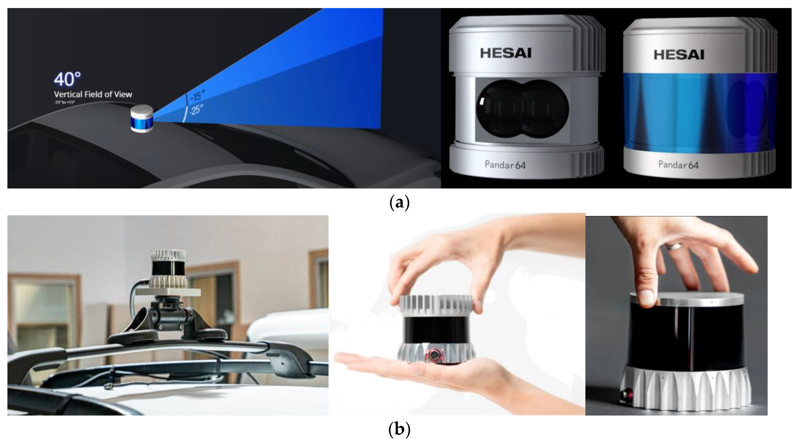
An investigation of two newly released state-of-the-art 64 channel Lidar types is applied to quantify the ideal angular orientation that fits for mobile mapping applications.

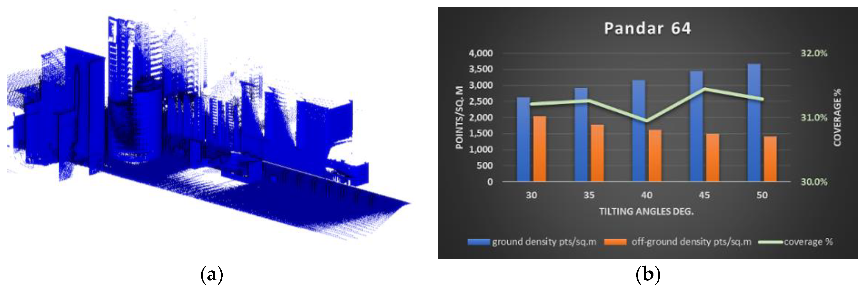
Both Lidar types are multi beam spinning Lidar types with 64 channels and represent a potential Lidar candidate for MMS especially with their reasonable size, weight, and cost. These two Lidars are lately released from different manufacturers in China and USA. The first Lidar is the Hesai Pandar 64 (Figure 1a) and the second Lidar is the Ouster OS-1-64 (Figure 1b).

Pandar64 has a longer maximum range of 200 m at 10% target reflectivity while having an irregular beams distribution or what may be called gradient distribution. On the other hand, Ouster OS-1-64 has a shorter range of 120 m @ 80% target reflectivity with linear distribution of beams and smaller beam divergence. The specifications of every Lidar type are summarized in

Table 1. Specifications of the investigated Lidar types.

Lidar Sensor/System	Ouster	HESAI
Type/version	OS-1 -64	Pandar64
Max. Range	≤120 m@80%	≤200 m@10%
Range Accuracy 1σ	±3 cm	±2 cm
Beam divergence	0.13° (2.2 mrad)	0.177° (3 mrad)
Output rate pts/sec.	≈1.3 million	≈1.15 million
FOV—Vertical	≈33.2° (±16.6°)	≈40° (+15°: −25°)
Rotation rate	10–20 Hz	10–20 Hz
Vertical resolution	0.53°	0.167°
Horizontal resolution	0.35° at 20 Hz	0.4° at 20 Hz
Number of beams	64	64
Lidar mechanism	Spinning	Spinning
Distribution of beams	Linear	Gradient
Weight	396 g	1.5 kg
Power consumption	20 W	22 W
Estimated cost price	≅$12 k	≅$30 k

, which shows that every type has its own advantages. Initially and based on the specifications, they are both suitable for high productivity mapping applications. A thorough investigation of their efficiency will be presented in Section 4.

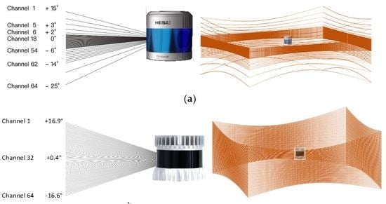
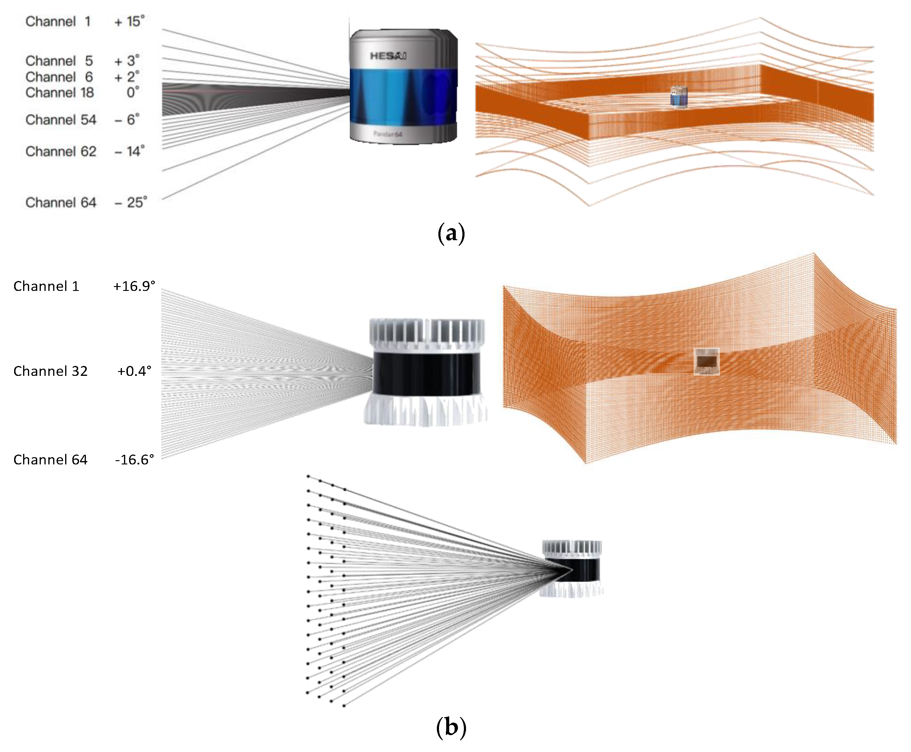
In Figure 2, the beam distribution pattern is given for both Lidars as published by their manufacturers [18,19]. Furthermore, to give the reader a visual impression about how the scans are expressed for each Lidar type, a simulation scanning space surrounded by walls is applied. Every Lidar type is placed at the center of the space, while the Lidar is placed on its base without a tilt in a stationary scan of one revolution.

2. Methods

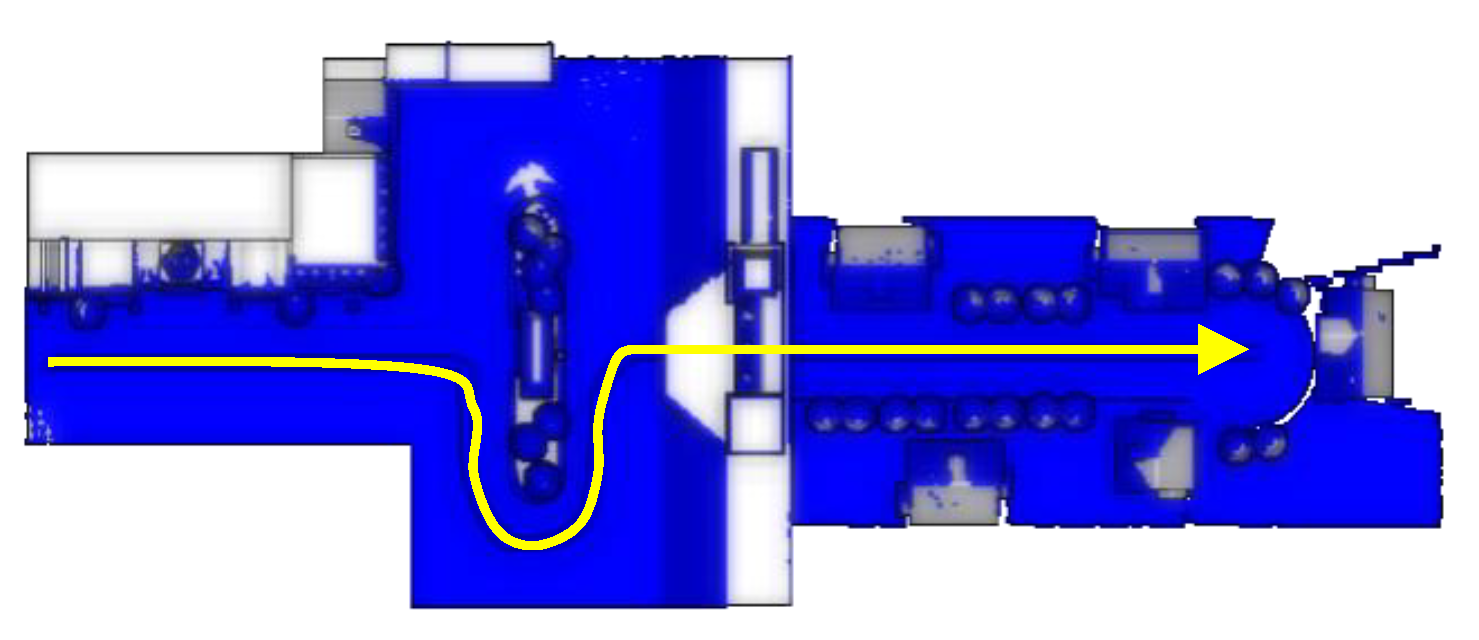
In this section, the method including evaluation parameters and simulation assumptions about the Lidar performance will be given. Namely, the angular orientations, scanning patterns, and the assessment of density, accuracy, and coverage. Figure 3 illustrates the methodology workflow. For both investigated Lidar types, the scanning routine is built based on the scanning properties given by the manufacturers. Then, a trajectory is defined in a 3D simulated urban model where a virtual mobile mapping system equipped with a single Lidar is mounted in a vehicle driving along the trajectory. It should be noted that the simulations are applied using the Blender tool [20].

In every run, a new tilting angle is initiated to orient the Lidar device and then a simulated scanning is applied. The produced point clouds in every angle set up is analyzed in terms of coverage, density, and accuracy and then a final performance evaluation is concluded.

2.1. Lidar Angular Set Up

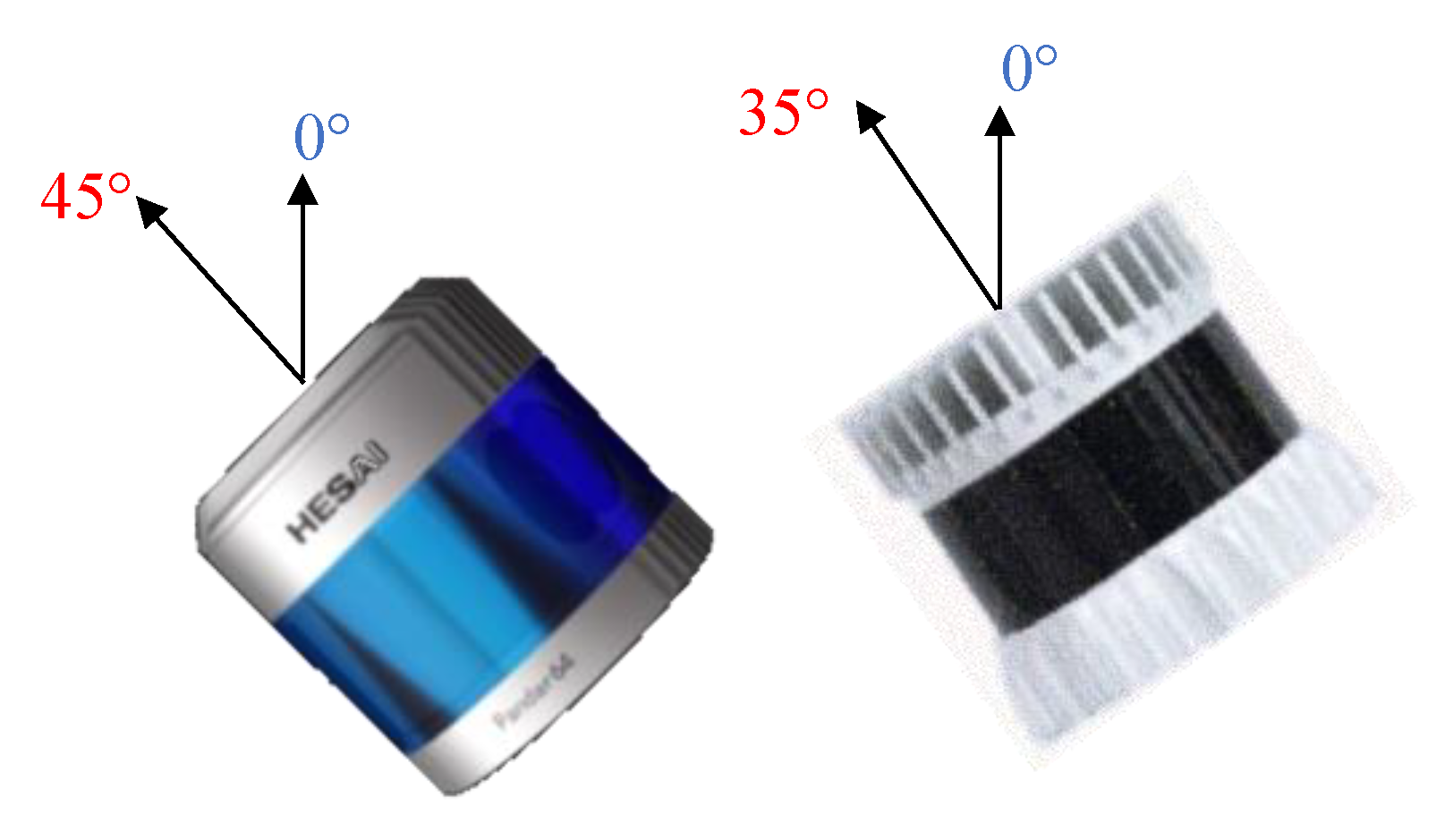
In this research paper, the ideal angular orientation of the two Lidar types is investigated to determine their suitability for the mobile mapping applications. The investigated angular range of the Lidar is defined as shown in Figure 4.

As shown in Figure 4a, the 0° tilting angle (blue color) is defined when the Lidar is placed on its base, and then the Lidar scanning lines will constitute concentric circles on the ground (Figure 4b). This 0° Lidar orientation is the mostly used in autonomous driving. On the other hand, when the Lidar is rotated 90° (red in Figure 4a), the scans will hit the ground surface close to right angles and result in a parallel scan line pattern (Figure 4b).

2.2. Accuracy Assessment

Accuracy assessment is an important measure to check the quality of the scanned objects at the different tilting angles of the Lidar. This estimation of accuracy can be achieved by applying the Lidar error model of Equation (1) [21]:

$$P_i^w\left(t\right)=M_{INS}^w\left(t\right)P_i^{INS}\left(t\right)+T_{INS}^w\left(t\right)$$

(1)

where $P_i^w\left(t\right)$ represents the 3D coordinate of a point $(X_i,Y_i,Z_i)$ in the world coordinate system at time $t$, $T_{INS}^w\left(t\right)$ is the position of the inertial navigation system INS in the world coordinate system at time $t$, $M_{INS}^w\left(t\right)$ is the rotation matrix between the INS body frame and the world coordinate system at time $t$, and $P_i^{INS}\left(t\right)$ is the position of the target point in the INS body frame at time $t$.

However, a pre-calibrated Lidar device is assumed in this study and as a result, errors in the lever arm offset, and boresight angles are assumed insignificant. Accordingly, the error propagation equation model is simplified where the position of every scanned point $X_i,Y_i,Z_i$ at time $t$ can be formulated as in Equation (2):

$$\begin{array}{l}{X}_i=X_1+Rcos\left(Az\right)cos\left(V\right)\\ Y_i=Y_1+Rsin\left(Az\right)cos\left(V\right)\\ Z_i=Z_1+Rsin\left(V\right)\end{array}$$

(2)

where $R$ is the measured range distance from the Lidar to the object point $P$, $Az$ is the measured azimuth angle of the laser beam, $V$ is the vertical angle of the laser beam measured from the horizon, and $X_1,Y_1$, and $Z_1$ are the coordinates of the Lidar sensor at $t$.

It should be noted that the errors of the Lidar coordinates $X_1,Y_1,Z_1$ are predicted in normal cases from an integrated INS. If the accuracy in the navigated Lidar coordinates is not included in the model of Equation (2), then the estimated errors of the scanned points will represent the relative accuracy.

An error propagation can be applied using Jacobian Matrix $J$ to estimate the errors of the scanned points in a point cloud as follows in Equations (3) and (4) [22]:

$$J=\left[\begin{array}{ccc}\frac{\partial Xi}{\partial Az}& \frac{\partial Xi}{\partial V}& \frac{\partial Xi}{\partial R}\\ \frac{\partial Yi}{\partial Az}& \frac{\partial Yi}{\partial V}& \frac{\partial Yi}{\partial R}\\ \frac{\partial Zi}{\partial Az}& \frac{\partial Zi}{\partial V}& \frac{\partial Zi}{\partial R}\end{array}\right]=\left[\begin{array}{ccc}-Rsin\left(A\right)cos\left(V\right)& -Rcos\left(A\right)sin\left(V\right)& cos\left(A\right)cos\left(V\right)\\ Rcos\left(A\right)cos\left(V\right)& -Rsin\left(A\right)sin\left(V\right)& sin\left(A\right)cos\left(V\right)\\ 0& Rcos\left(V\right)& sin\left(V\right)\end{array}\right]$$

(3)

$${\displaystyle \sum }_{XYZ}=J{\displaystyle \sum }_{R,Az,V}{J}^t=\left[\begin{array}{ccc}{\sigma }_{Xi}{}^2& & \\ & {\sigma }_{Yi}{}^2& \\ & & {\sigma }_{Zi}{}^2\end{array}\right]$$

(4)

where ${{\displaystyle \sum }}_{R,Az,V}$ is the variance-covariance matrix of the scanned range and angles to the point cloud, ${{\displaystyle \sum }}_{XYZ}$ is the variance-covariance matrix of the derived coordinates of the point cloud, ${\sigma }_{Xi},{\sigma }_{Yi},{\sigma }_{Zi}$ are the standard deviations of point $i$ coordinates, and $t$ is the matrix transpose.

For illustration, exaggerated ellipsoids of errors are shown in Figure 5 for the scan sweep at 30° of a multi beam Lidar on the ground. Figure 5 illustrates how errors are larger for scanned ground points at longer scanning ranges away from the Lidar.

2.3. Density Assessment

Computing the point density is one of the performance evaluation categories in this paper and it describes the number of points in one squared meter (pts/m²). The density computation will be applied simply by finding the nearest neighbor points of every scanned point within a searching radius and sort their number as density.

As there will be a definite opportunity for having empty space between measurements, it is also possible to describe density by the point spacing [23]. Spacing between points can be calculated from the density as in Equation (5) [16]:

$$samplespacing=\sqrt{\frac{1}{pointdensity}}$$

(5)

However, this simple equation assumes a uniform distribution of points which is not the case with the two Lidar types under investigation. Worth to mention is that in this paper, point clouds were simulated assuming one pulse return and this also complied with the US Geological Survey standards.

2.4. Coverage Assessment

Coverage or completeness is one of the important quality measures of point clouds. Although this is a difficult to define task for ground-based mapping systems, it is possible to assess in this paper, since the reference simulated urban 3D model is well defined.

The coverage percentage is computed by subtracting the scanned point cloud (blue color) from the reference model point cloud (gray color) as shown in Figure 6. First, the proximity between the scanned points and the reference evenly spaced points were computed. Then, only assigned points in the reference point cloud were considered for assessing the coverage against the whole reference point cloud.

2.5. Scanning Pattern Assessment

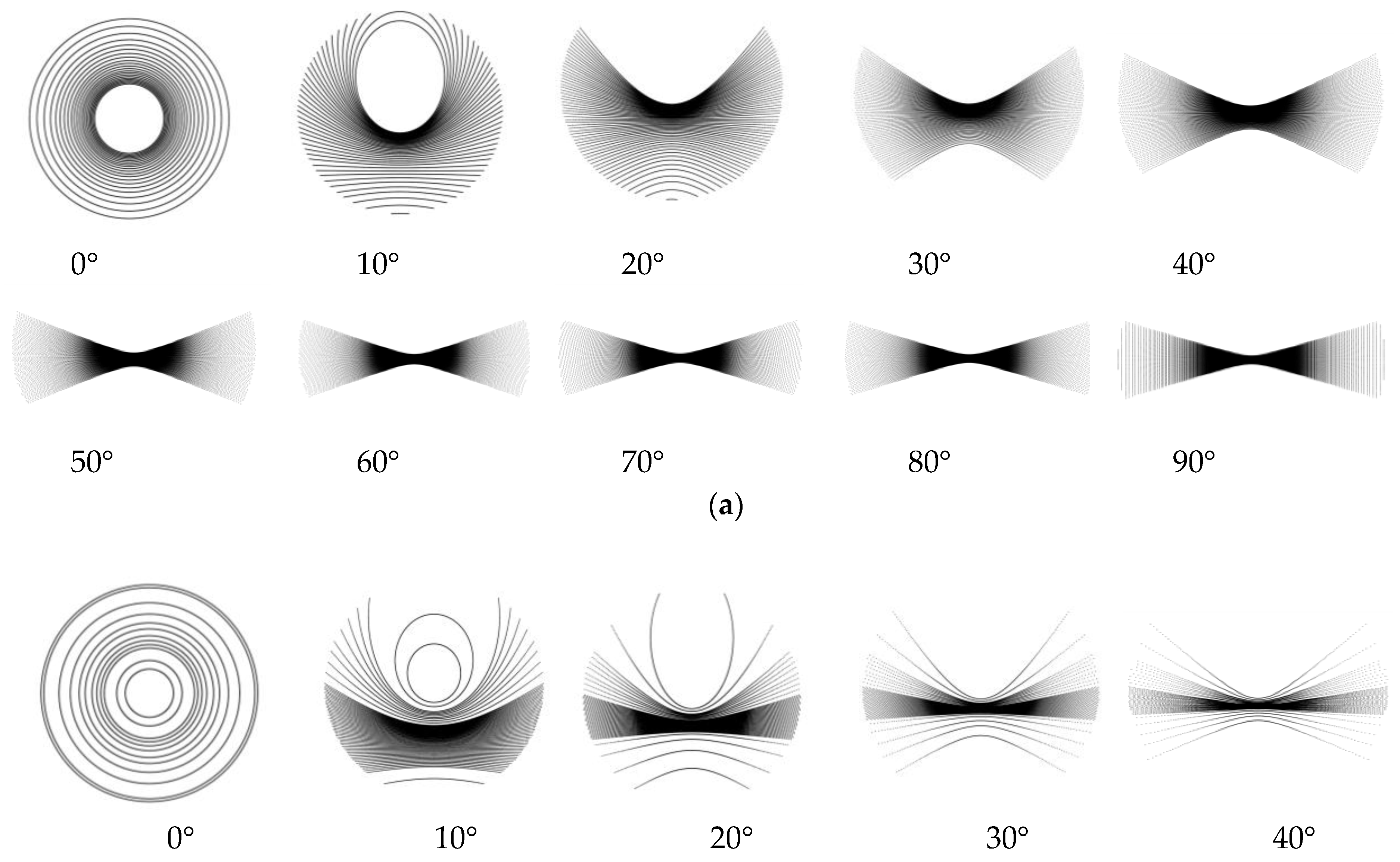
To decide which orientation angels can be investigated in the experiment of the two Lidar types, we applied a scanning simulation at an angular range of 0°–90° at a 10° interval. This is simply simulated by placing every Lidar at 2 m height in an MMS where a revolution scan is applied to a planar ground and a façade (Figure 7).

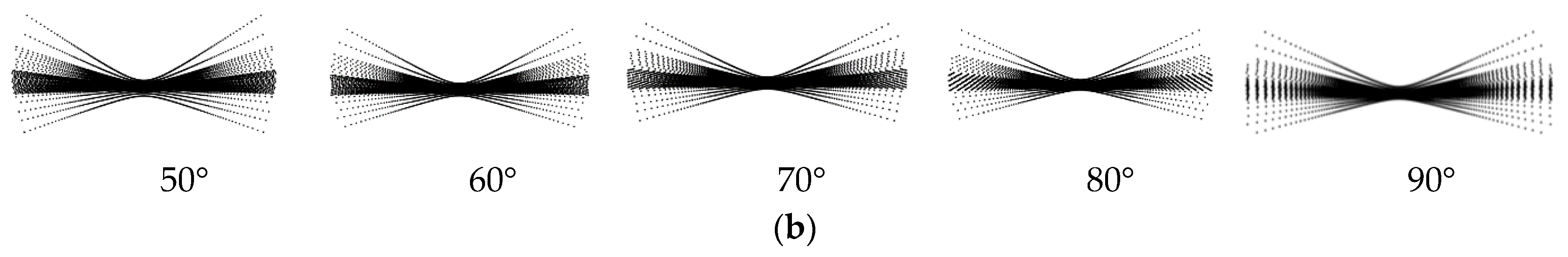
The pattern of a stationary scanning sweep on the ground for the two Lidar types of the selected tilt angles from 0°–90° is shown in (Figure 8) with a scanning range of 20 m.

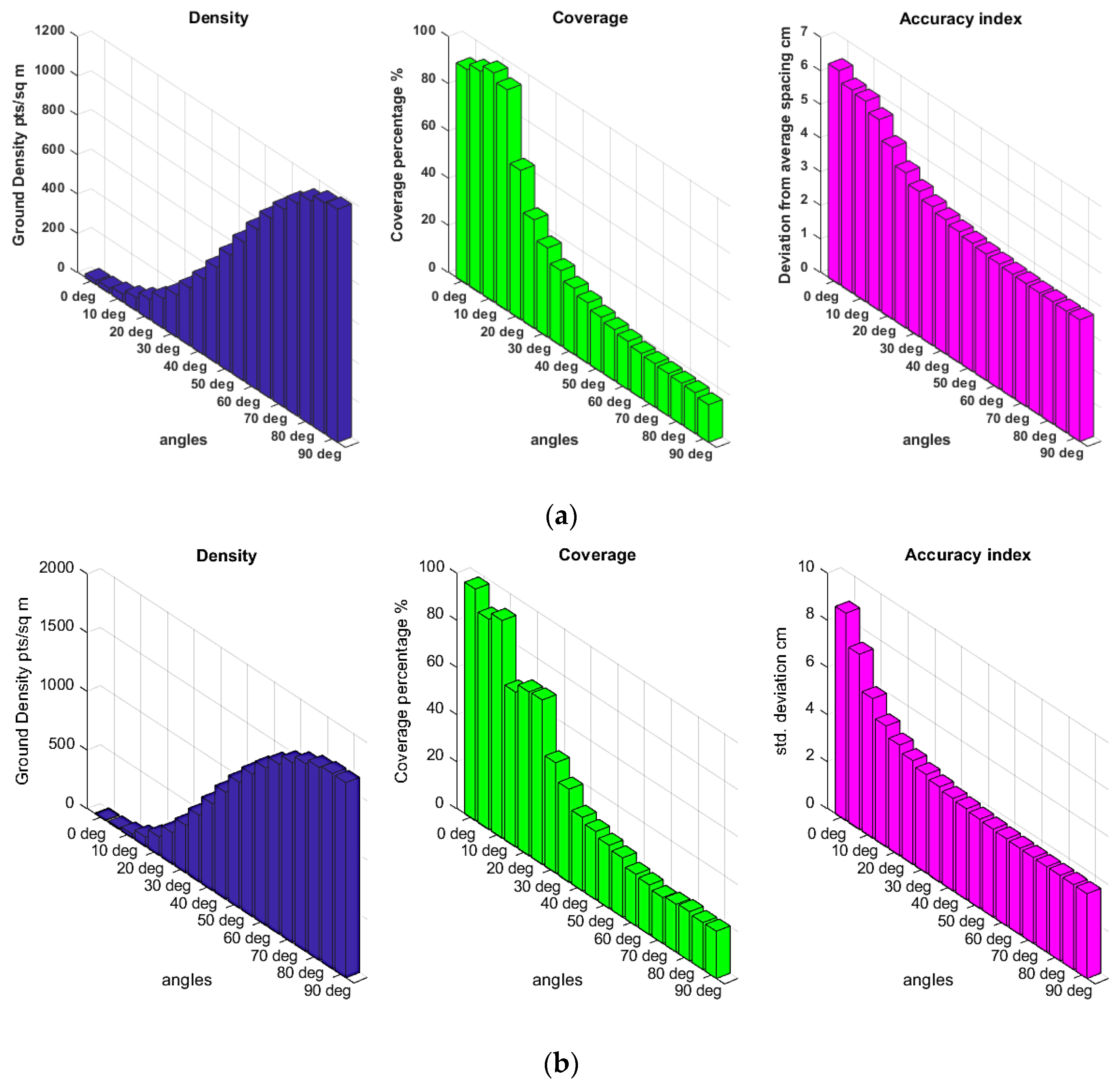
Both Lidar types scanning patterns shown in Figure 8 are analyzed in terms of density, coverage, and accuracy to get the performance histograms shown in Figure 9.

A slight difference between OS-1-64 and Pandar64 is found in the coverage aspect. Whenever the tilt angle increases greater than 10°, OS-1-64 coverage scanning footprint decreases. On the other hand, for Pandar64, the coverage area decreases constantly when the tilting angle is greater than 25°. This might be related to: (a) the symmetry of the vertical FOV around the horizon and (b) the distribution pattern of the beams as illustrated in Figure 2. On the other hand, both Lidars have the same behavior for density and accuracy magnitudes. What can be clearly identified from the histograms in Figure 9 is the inverse relation between the density and accuracy on one side versus coverage from the other side. Accordingly, a compromise of these contradicting properties has been decided by considering the tilting angle range of 30°–50°. This angular orientation range is in general the most suitable for experimenting and evaluating the two Lidars performance for mobile mapping applications as will be presented in Section 4.

3. Experiment Design

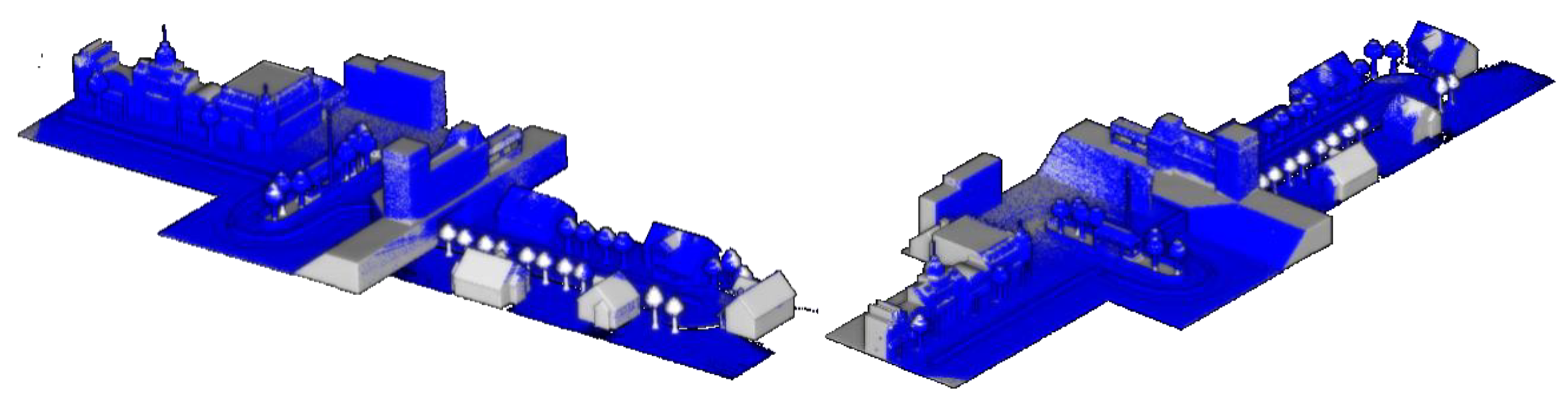
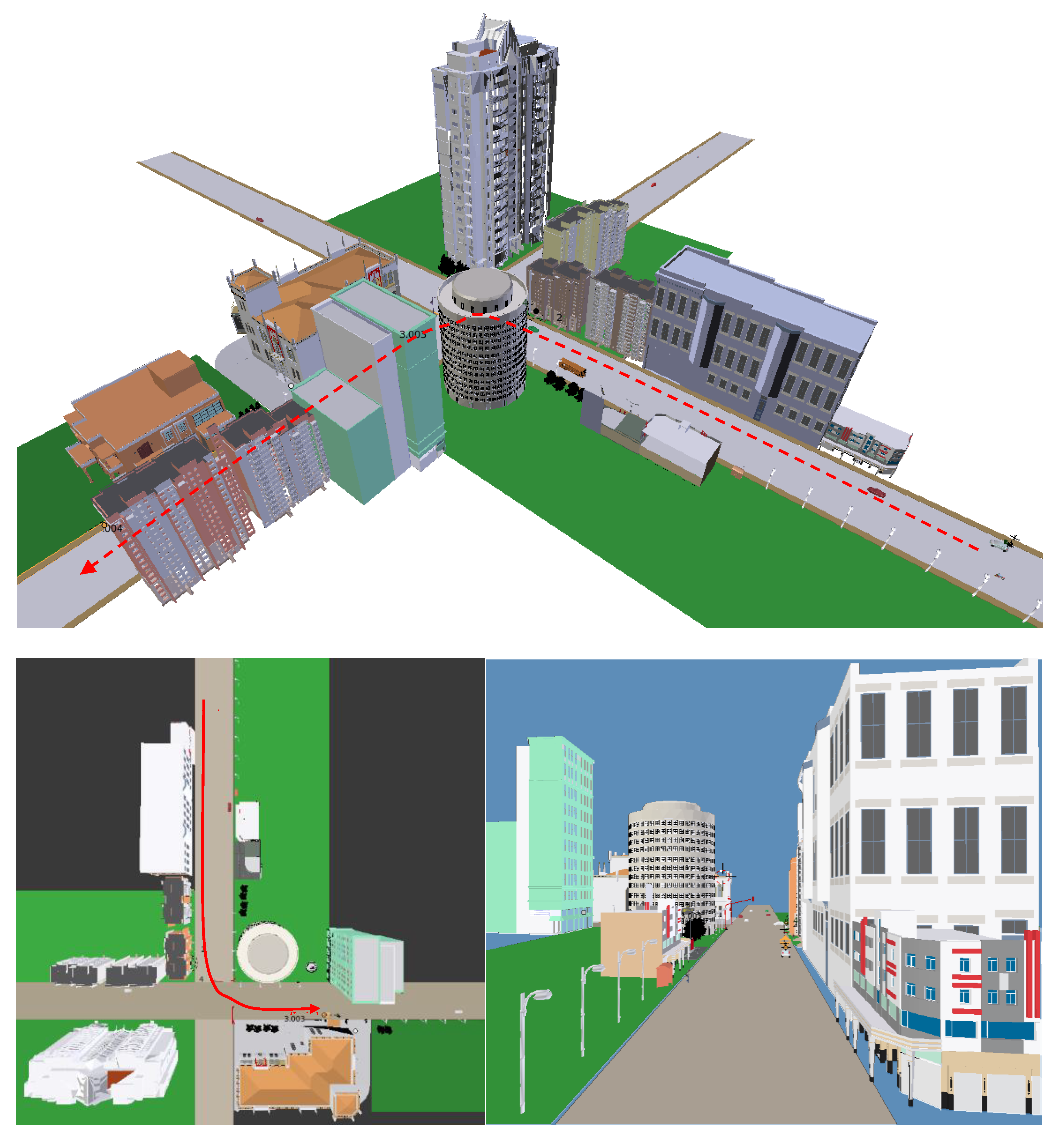
The experimental test was applied in a simulated urban environment (Figure 10) where different buildings, light poles, traffic lights, moving cars, and trees are existed. The simulated drive was applied to a mobile mapping system equipped with the mentioned 64-channel Lidars of OS-1-64 and Pandar64 at a height of 2 m above the ground with a constant driving speed of 36 km/h.

Five tilting angles of 30°, 35°, 40°, 45°, and 50° were investigated in the scanning for both Lidars. It should be noted that the simulations omitted any limited FOV and the existence of occlusions that might occur because of the vehicle body or the camera system itself and assumed a perfect occlusion-free mobile mapping system.

The accuracy evaluations of the two Lidars are represented by standard deviations derived in the propagation of error as described in Section 2.2. A standard deviation of ±3 cm in range and ±0.1° in angles were used in the calculations related to the manufacturers’ specifications.

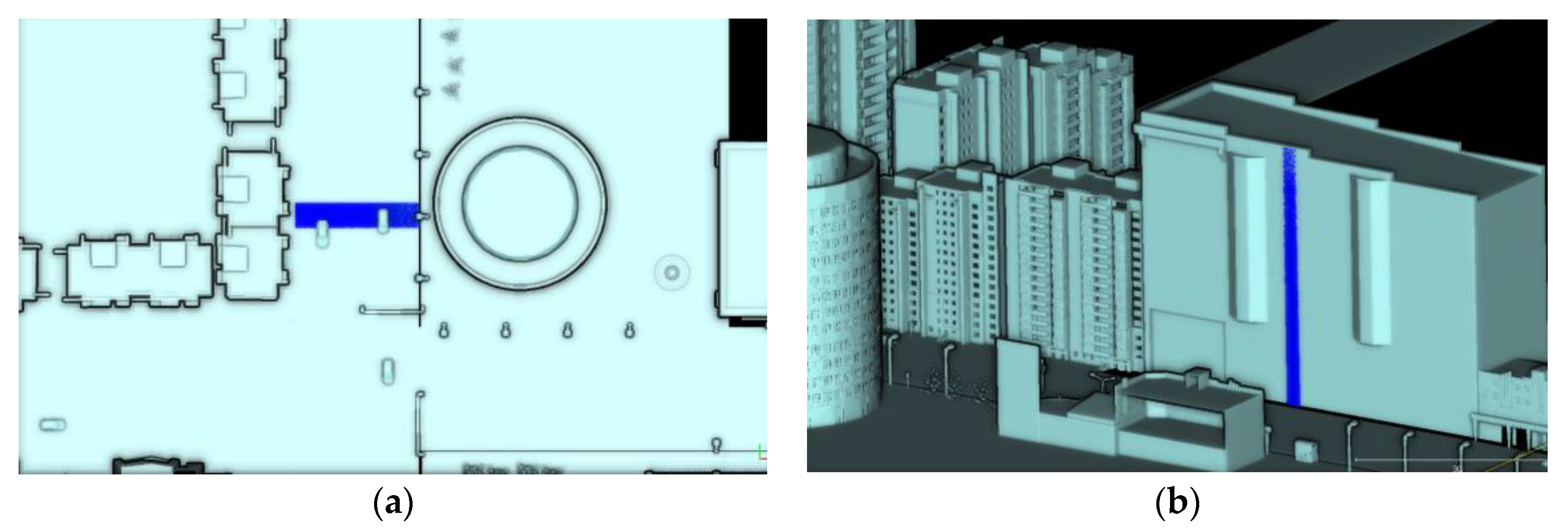
Two density checks are applied: (1) overall ground and off ground density check using the CloudCompare tool [24]; (2) density check on two selected slices on the ground (20 m length) and off ground (40 m height) as shown in Figure 11. The density tests are applied for all the aforementioned tilting angles of both Lidars as will be shown in Section 4.

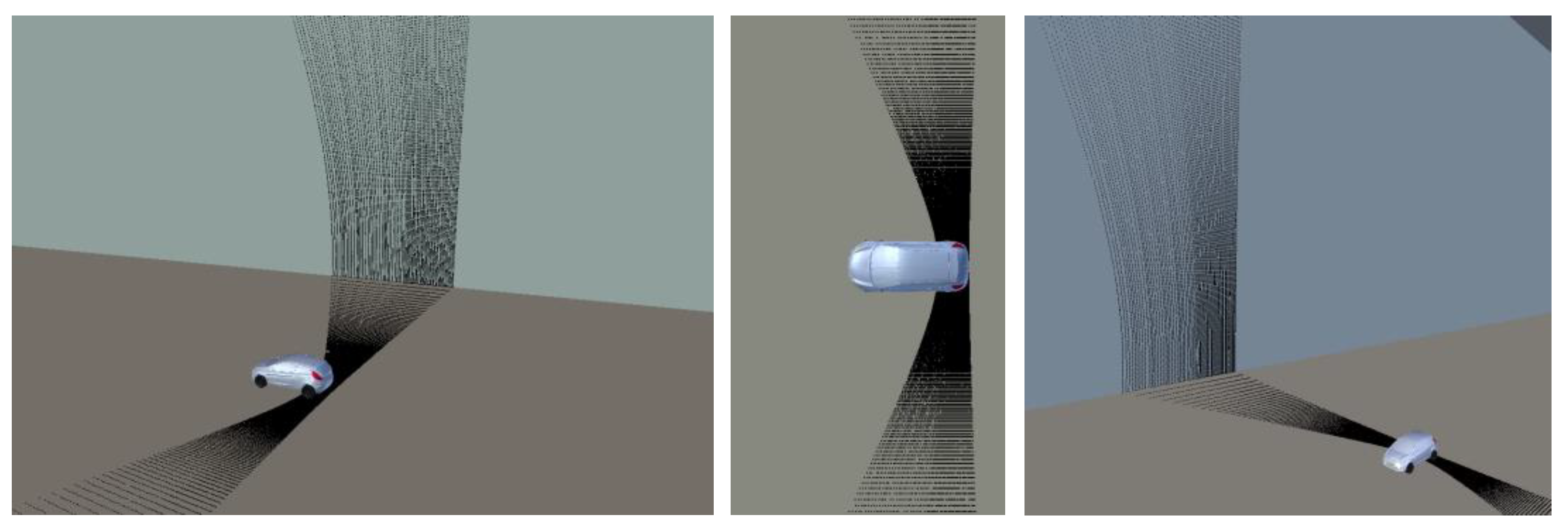
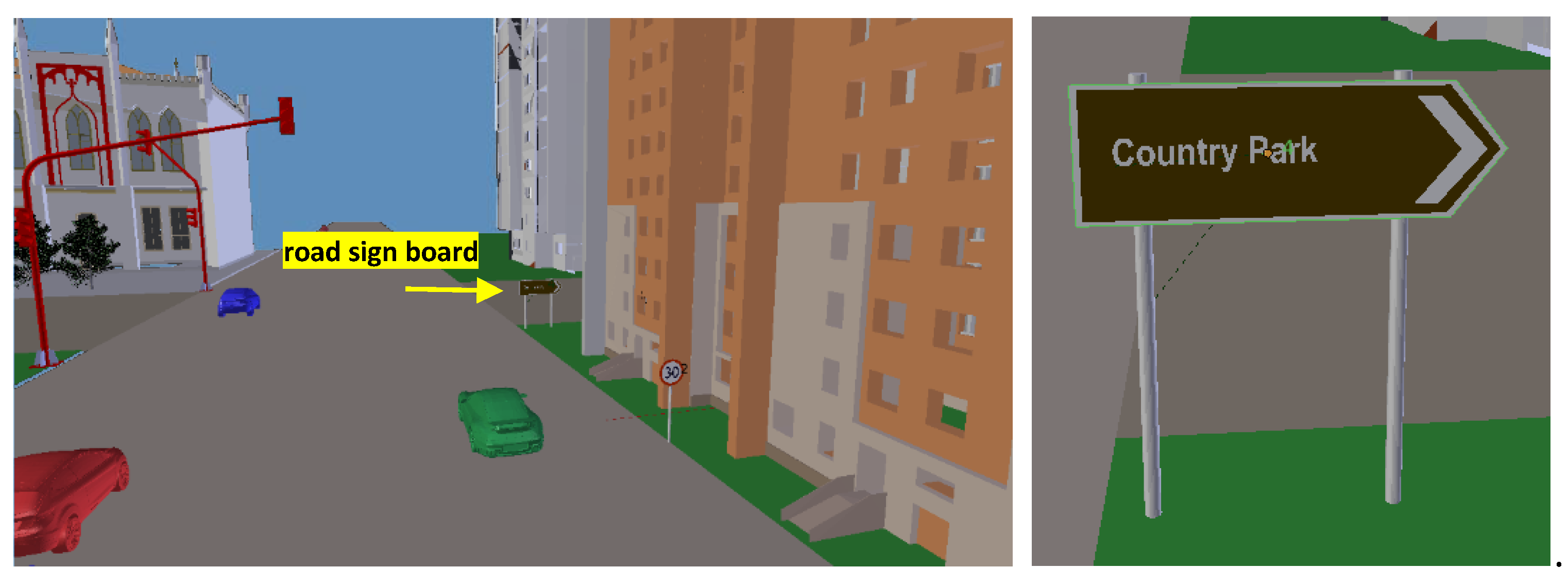
A third test type was applied to check the density achieved on a traffic board sign located at distance of five meters from the trajectory, which increased as the car turned to the left road in the driving scenario (Figure 12). The test checked the effectiveness of cylindrical posts detection at the different tilting angles for the two Lidar types.

4. Results

In this section, the performance evaluation of the two Lidar types OS-1-64 and Pandar64 will be shown by a simulated drive with an MMS equipped with one Lidar device each time. The simulations are applied using the same trajectory and a constant vehicle speed of 36 km/h. It should be noted that we did not apply simulations at different driving speeds because of the linear dependency between the produced point clouds data and the mapping vehicle speed.

4.1. Simulation Results of Pandar64

For every tilting angle of 30°, 35°, 40°, 45°, and 50°, the point cloud density was computed on both the ground and off ground. The results are represented as shown in Figure 13, where the density increases on ground features whenever the tilting angle increases.

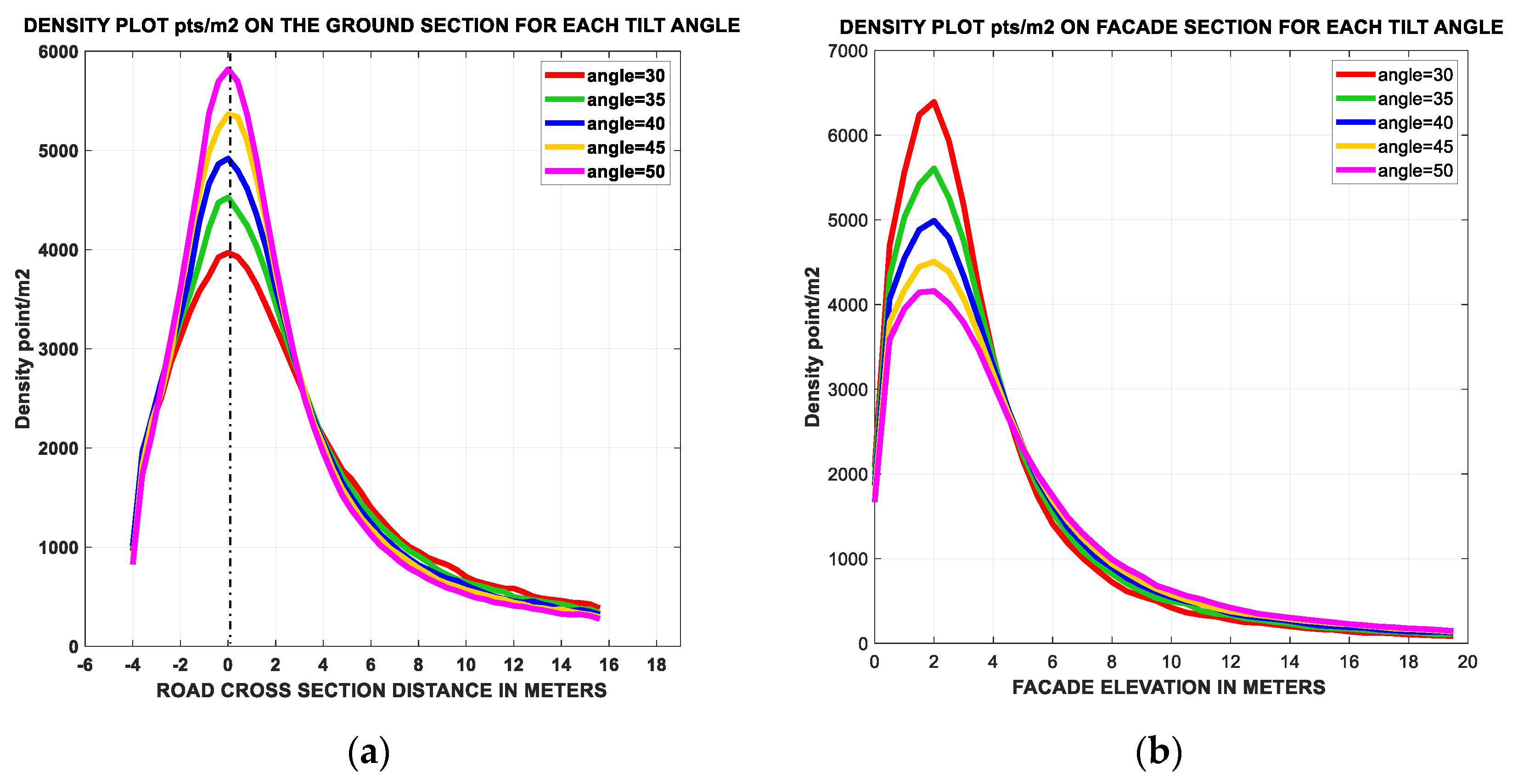
The density check on the selected slices of Figure 11 was also evaluated and represented in Figure 14. It should be noted that the façade slice was 5 m away from the mapping trajectory.

It should be noted that the 0 value of the x-axis indicates the scanning trajectory on the ground section in Figure 14a, while the start elevation of the façade section is shown in Figure 14b. For facades, higher densities are achieved up to a height of 4 m, and then drops quickly whenever the elevation increased. While the high scanning density on the ground (≈2000 pts/m²) is achieved within 8 m road width.

A large produced amount of data is shown in Figure 13 and Figure 14 in terms of the achieved density of the point clouds at every tilting angle. This amount of density, if the achieved accuracy is not counted, is highly suitable for engineering surveys, asset management inventory, roadway condition assessment, powerline clearance, 3D designs, as built surveys, and other general mapping applications, as indicated in [16].

Coverage percentage was evaluated by comparing the resulted point cloud at each tilt angle to the reference model (Figure 15). The coverage was found to be slightly fluctuating as shown in Figure 13, where it starts at a high percentage of 30°, decreases at 40°, and then improves at 45°. However, the difference is within 0.25%.

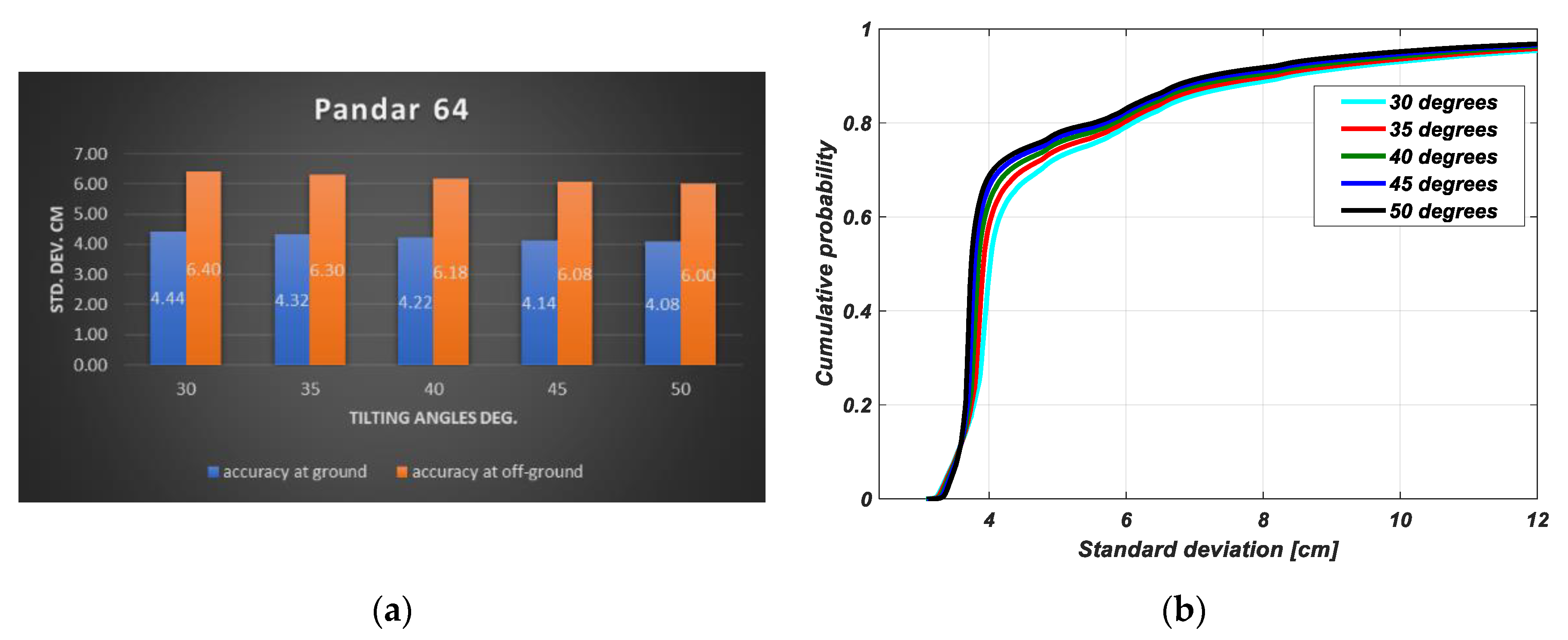
As mentioned earlier, the third parameter for the performance evaluation is the accuracy in the positions of the scanned points. Relative accuracy computed on both the ground and off ground features, and was found to improve whenever the tilting angle increased, as shown in Figure 16a. Furthermore, to illustrate the predicted accuracy at every tilting angle, a cumulative distribution function CDF chart [21] is plotted for the whole point clouds in Figure 16b.

The CDF chart shows the accuracy of the point cloud at each tilting angle using Equation (4). A better accuracy is achieved at larger tilting angles, which is logical since the incident angles of the laser beams are getting closer to right angles at the road surface and facades at the trajectory sides.

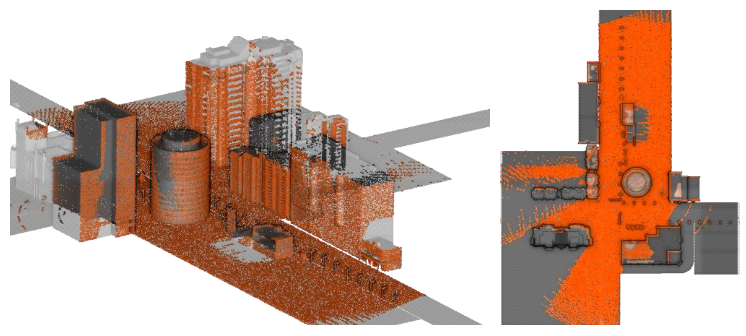
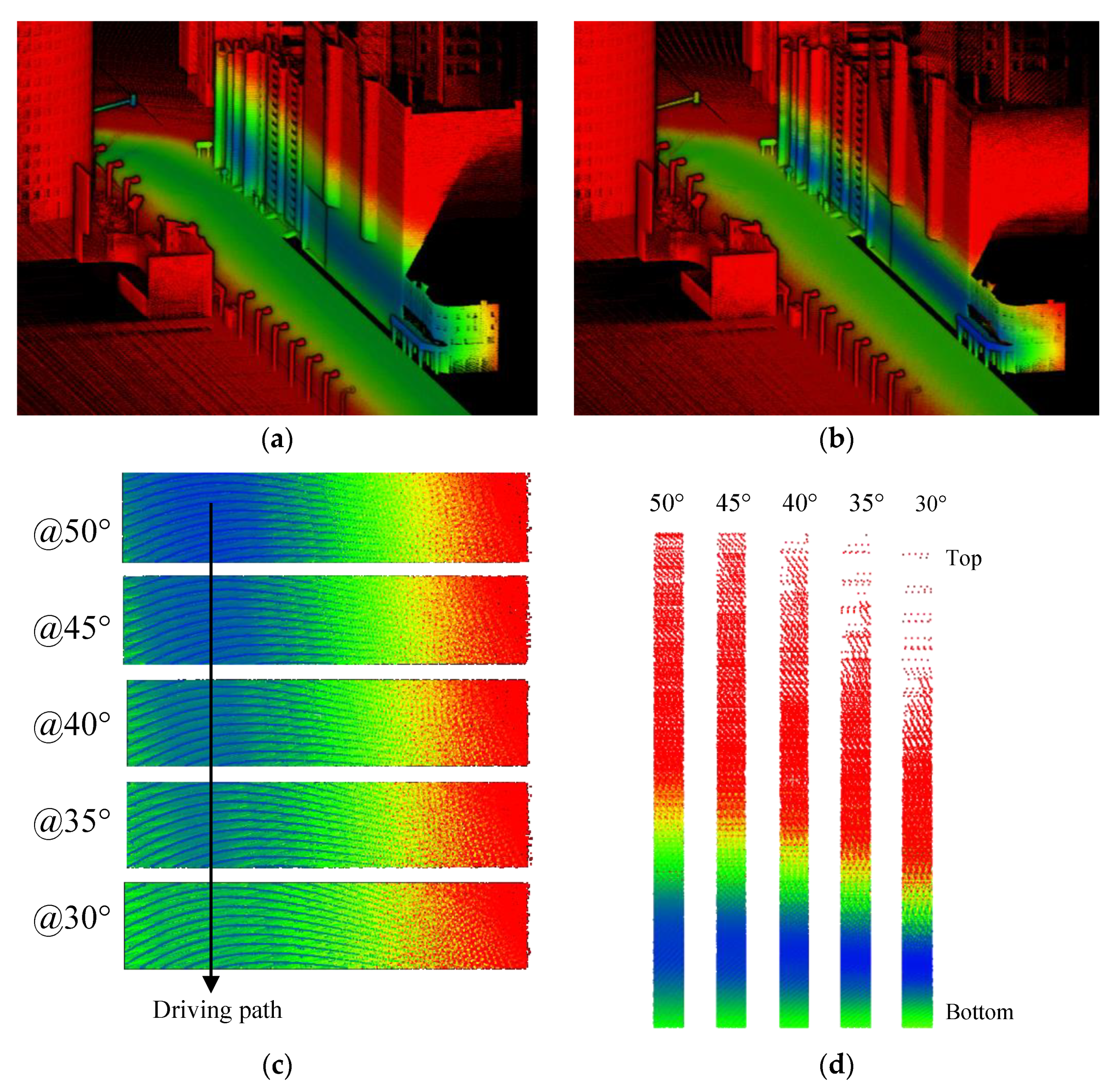
The estimated accuracy at 50° and 30° Lidar tilt angles is illustrated in Figure 17a,b, respectively, where every point with ≥5 cm standard deviation in position is colored red. For a better illustration, the point clouds were also tested for both selected slices of Figure 11 on the ground and on the façade. Figure 17c,d show the estimated accuracy at every Lidar tilting angle for both testing slices, where the points that have a standard deviation ≥5 cm are colored red. The summarized average standard deviations at both testing slices are listed in

Table 2. The estimated average standard deviation on the ground and facade slices using Pandar64.

	Average Standard Deviation [cm]
Lidar Tilt Angle	Façade Slice	Ground Slice
50°	3.75 ± 0.95	3.82 ± 0.42
45°	3.76 ± 1.03	3.87 ± 0.46
40°	3.76 ± 1.06	3.93 ± 0.51
35°	3.75 ± 1.08	4.01 ± 0.58
30°	3.76 ± 1.13	4.12 ± 0.68

.

The plots show a higher relative accuracy at the 50° angle compared to the 30° angle. This difference in accuracy is clearly related to the incidence angle of the scanning beams as mentioned.

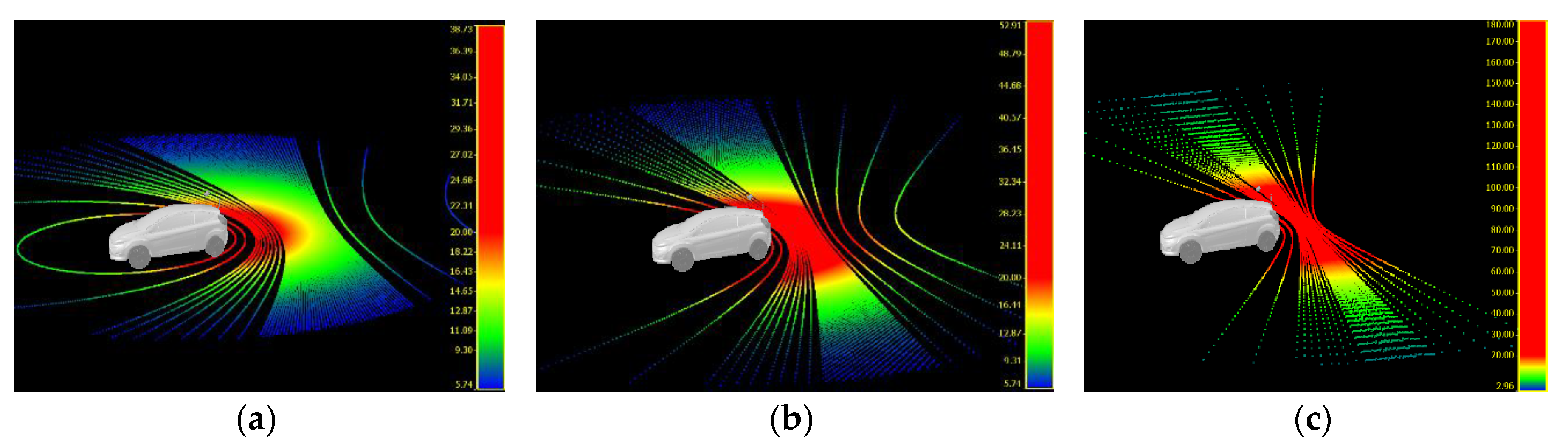
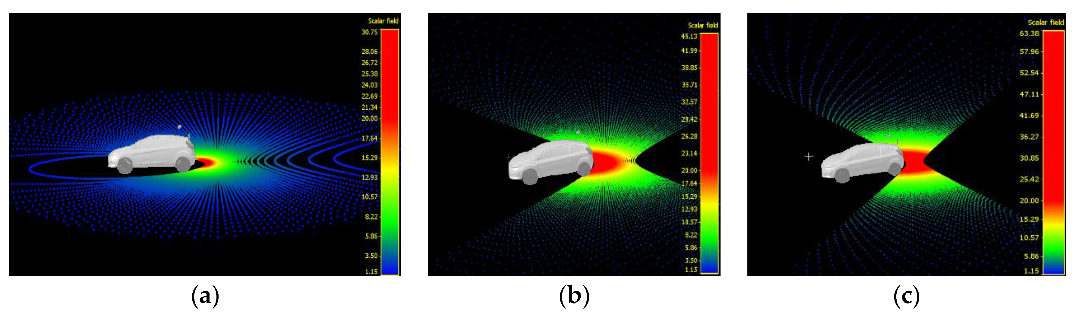
Figure 18 illustrates examples for the incidence angle magnitudes achieved on the ground at three different Lidar tilting angles of 15°, 30°, and 50°. The figure illustrates how the increase of the laser beams incidence angles on the ground is related to the increase of the Lidar tilt angle.

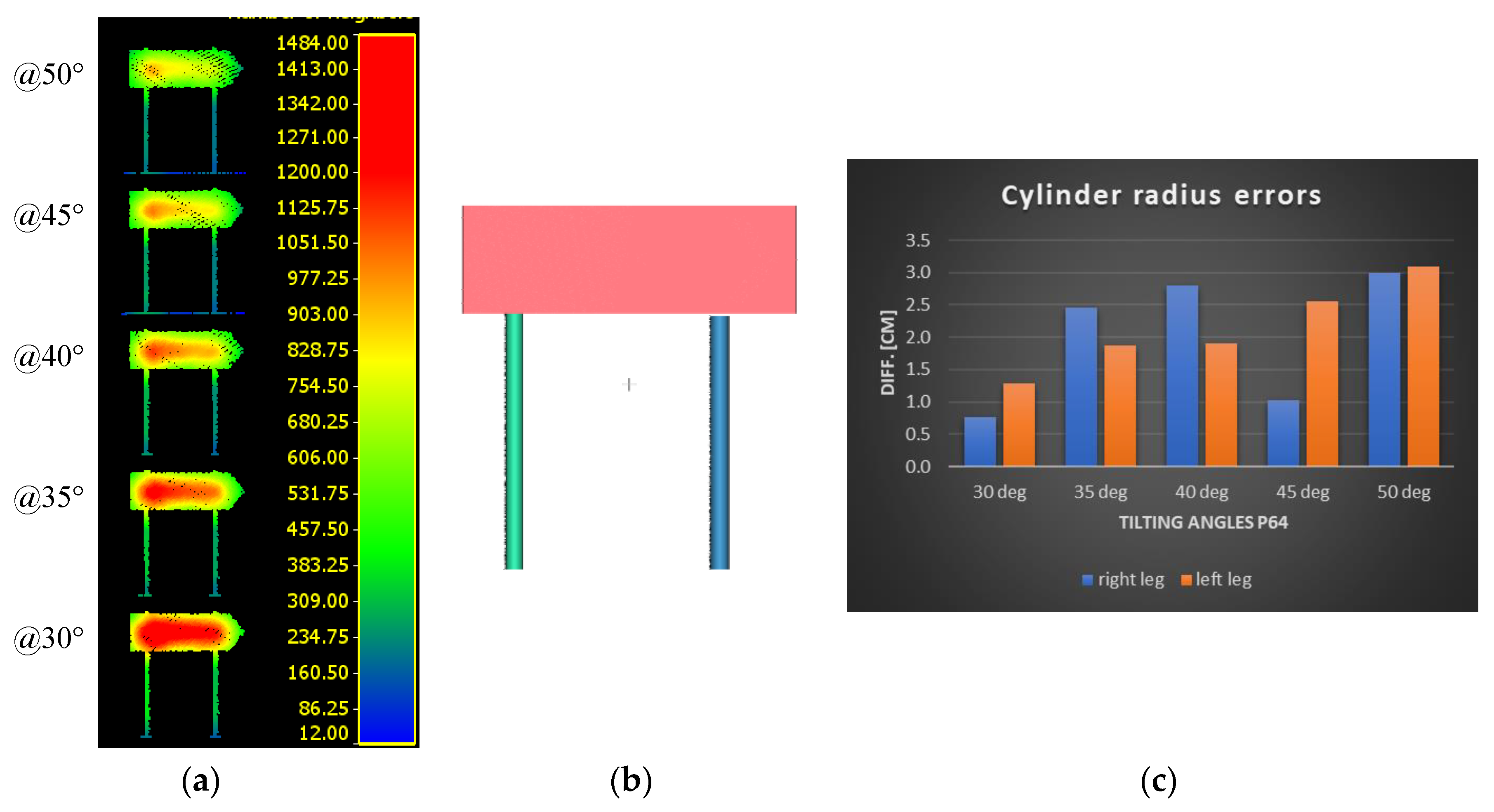
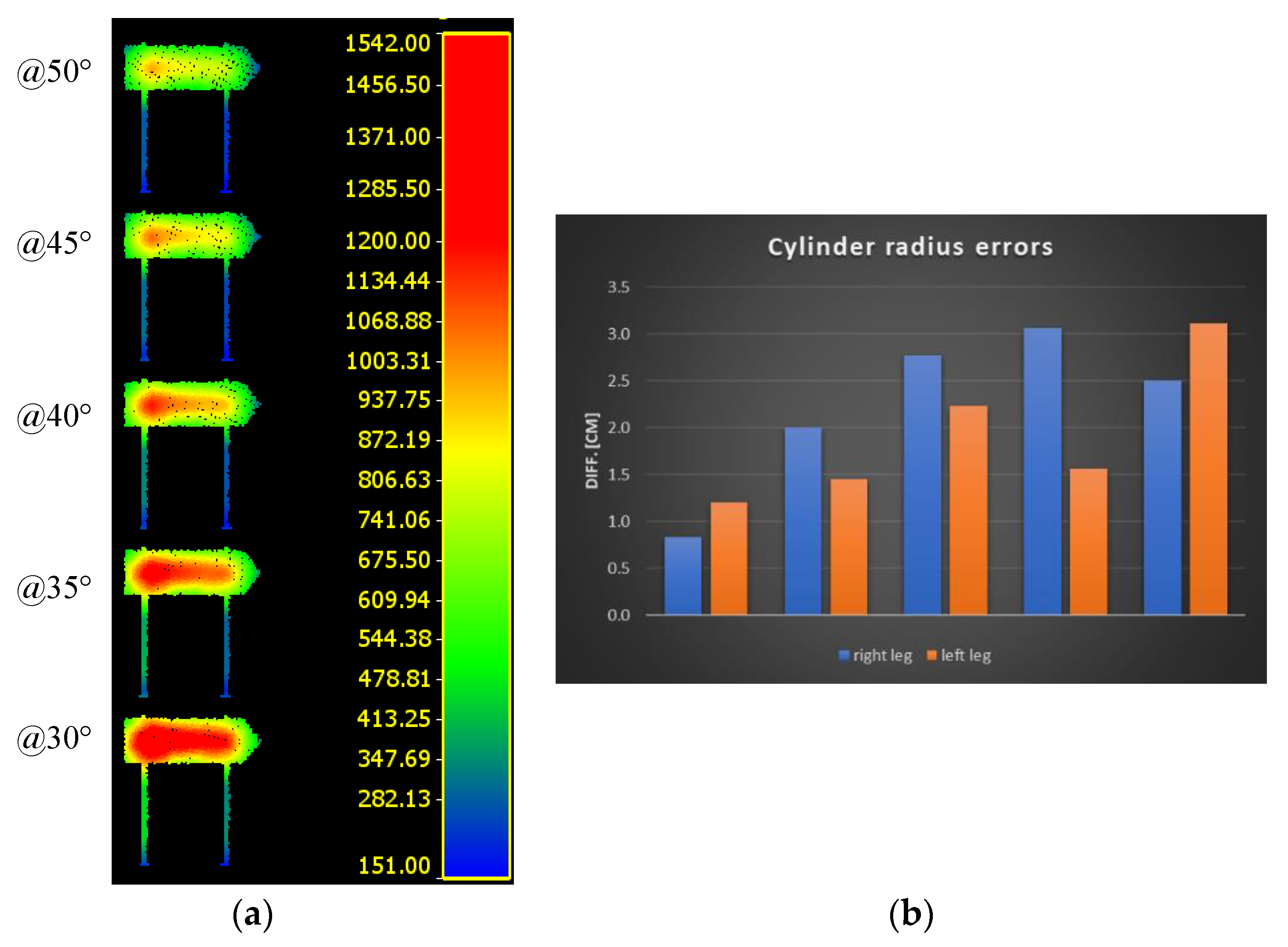
The third test as mentioned is to test the scanning goodness of a traffic sign at a road corner (Figure 12). Traffic sign test shows that the average number of scan points is decreasing from an average of 838 pts/m² at 30° tilt angle to 507 pts/m² at 50° tilting angle (Figure 19a). CloudCompare Ransac shape detection plugin is used to detect the sign cylindrical legs geometric primitives (Figure 19b). Accordingly, the deviation of the two detected cylindrical legs radii is computed with respect to the reference model radius (Figure 19c).

Assuming good set up parameters were entered for the cylinder fitting algorithm, we can say that, except for the point cloud produced at 30° tilt, the cylinder fitting at the other angles produced extra small cylinders as a false positive detection.

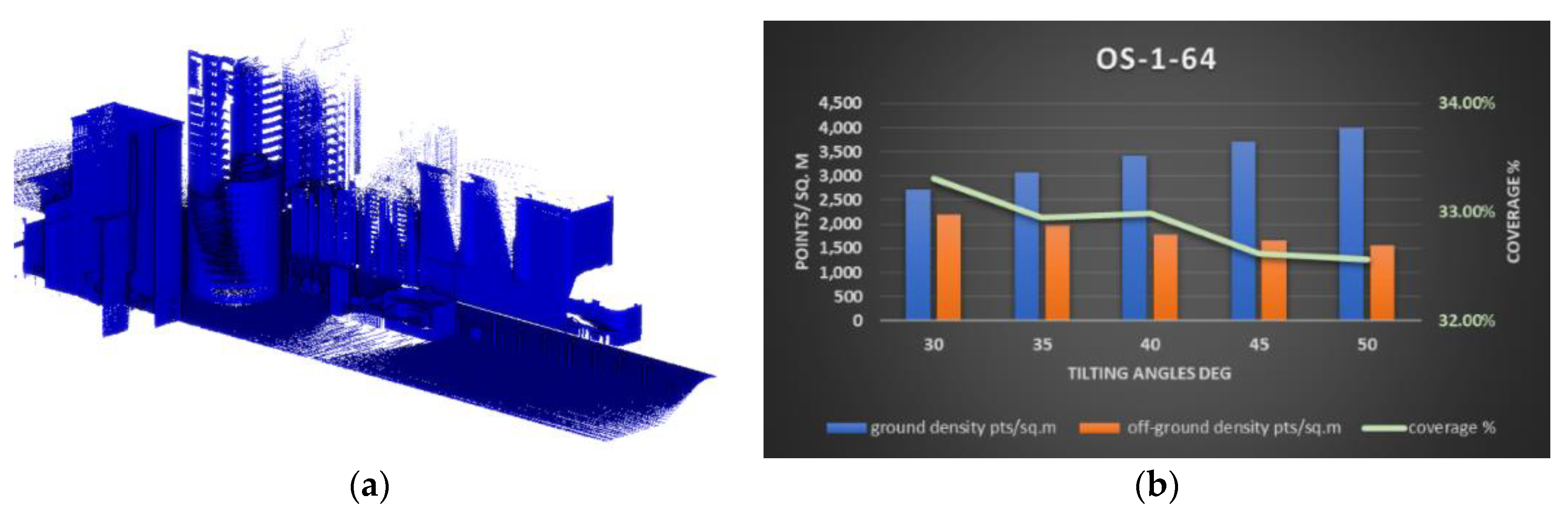
4.2. Simulation Results of OS-1-64

Similar to the tests applied for Pandar64 in Section 4.1, density was computed for the point clouds produced from OS-1-64 for every tilting angle at 30°, 35°, 40°, 45°, and 50°. The point cloud density was computed on both the ground and off ground. The results are shown in Figure 20, where the density increases on ground features whenever the tilting angle increases.

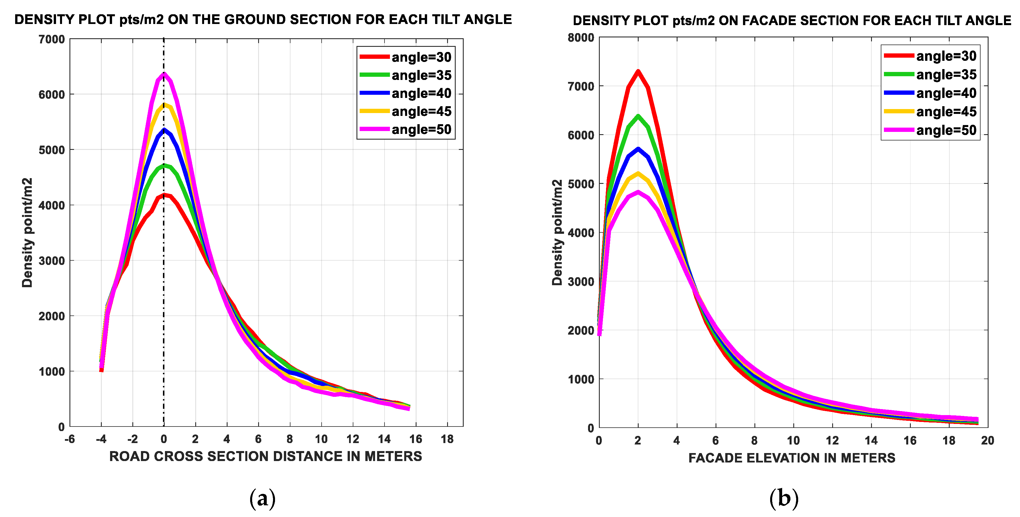
The density check on the selected slices of Figure 11 is also evaluated and represented in Figure 21. It should be noted that a 0 value on the x-axis indicates the scanning trajectory on the ground section in Figure 21a, while the start elevation on the façade section is shown in Figure 21b.

Figure 20 and Figure 21 indicate a large produced amount of data in terms of the achieved density of the point clouds at every tilting angle.

Furthermore, coverage percentage is evaluated by comparing the resulted point cloud at each tilt angle to the reference model. The coverage is found to be decreasing as shown in Figure 20 whenever the tiling angle increases.

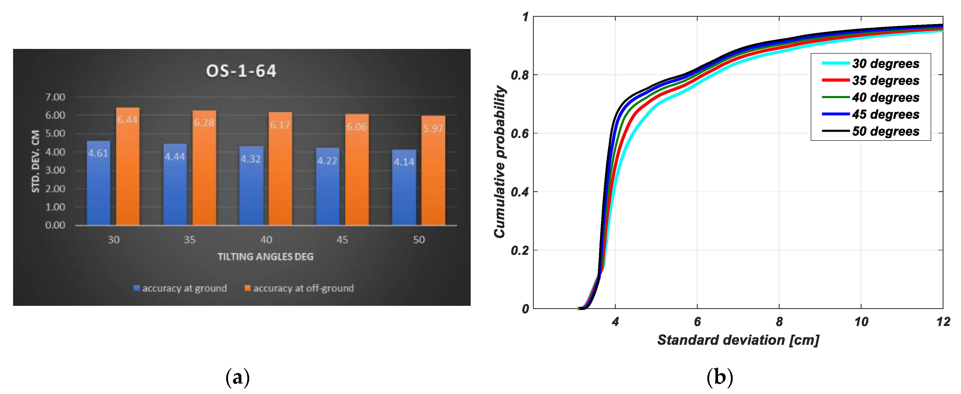
The performance evaluation in terms of accuracy in the positions of the scanned points was also applied for the point clouds produced by the OS-1-64. Similar to the Pandar64 case, relative accuracy computed on both ground and off ground features was found to be improving whenever the tilting angle increased, as shown in Figure 22a. Furthermore, to illustrate the accuracy predicted at every tilting angle, a CDF chart was plotted for the whole point clouds in Figure 22b.

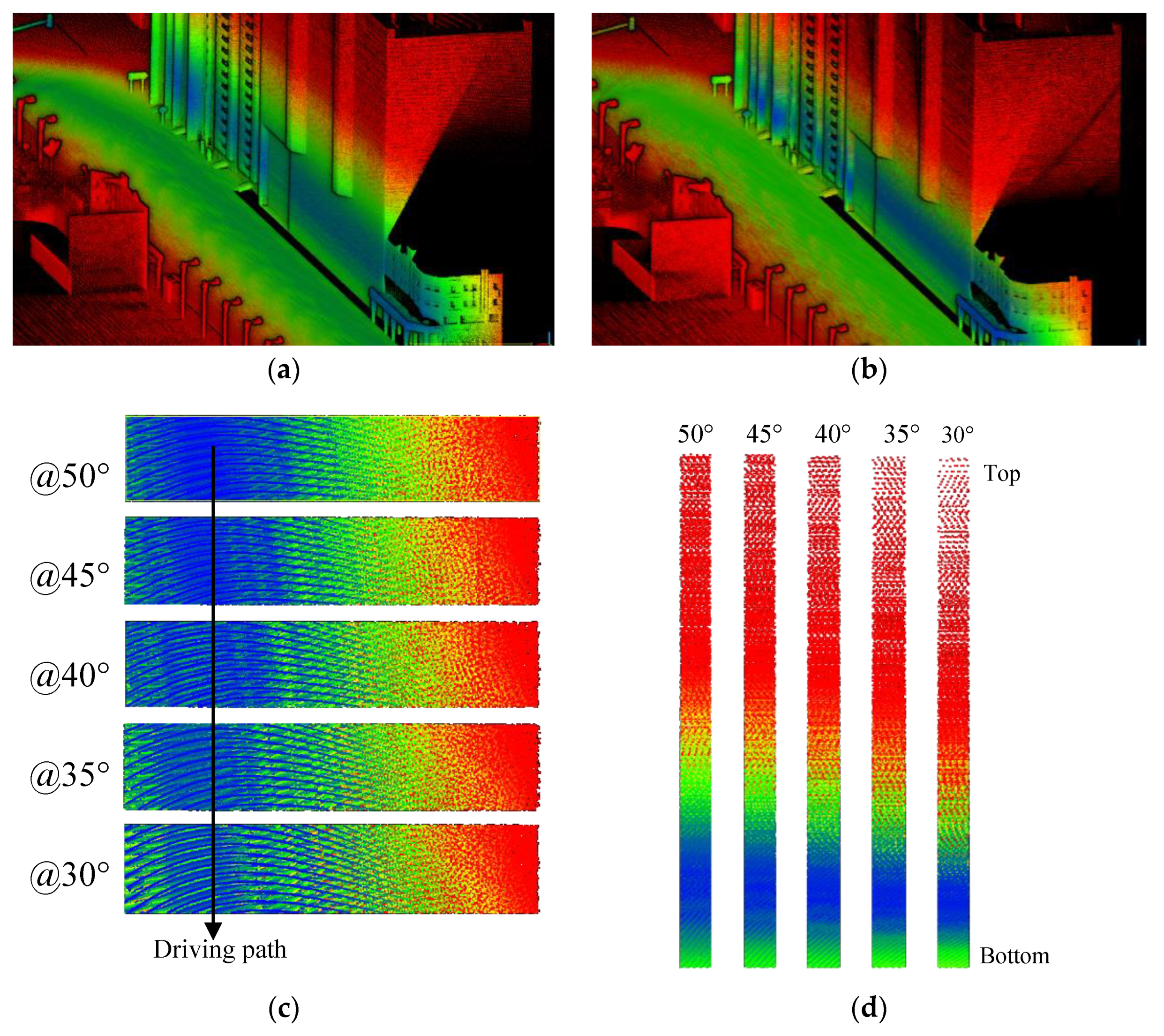
The CDF chart shows the accuracy of the point cloud at each tilting angle using the error propagation described in Section 2.2. The estimated accuracy at 50° and 30° Lidar tilt angles is illustrated in Figure 23a,b respectively, where every point with ≥5 cm standard deviation in position is colored red. For a better illustration, the point clouds were also tested for both selected slices of Figure 11 on the ground and on the façade. Figure 23c,d show the estimated accuracy at every Lidar tilting angle for both testing slices. The summarized average standard deviations at both testing slices are listed in

Table 3. The estimated average standard deviation on the ground and facade slices using OS-1-64.

	Average Standard Deviation [cm]
Tilt Angle	Façade Slice	Ground Slice
50°	3.85 ± 1.62	3.91 ± 0.86
45°	3.87 ± 1.75	3.99 ± 0.97
40°	3.88 ± 1.85	4.08 ± 1.09
35°	3.91 ± 1.94	4.20 ± 1.30
30°	3.95 ± 2.08	4.37 ± 1.53

.

This difference in accuracy at each Lidar tilt angle is clearly related to the incidence angle of the scanning beams. Figure 24 illustrates examples for the incidence angle magnitudes achieved on the ground at three different Lidar tilting angles of 15°, 30°, and 50°.

As explained, the third test is to evaluate the scanning efficiency on a traffic sign at a road corner (Figure 12). Traffic sign test shows that the average number of scan points is decreasing from an average of 848 pts/m² at 30° tilt angle to 539 pts/m² at 50° tilting angle (Figure 25a). The deviation of the two detected cylindrical legs radii is computed with respect to the reference model radius and shown in Figure 25b.

Similar to the observation mentioned using Pandar64, the point cloud produced at 30° tilt angle is more suitable in the sense of less fitting errors and detection.

5. Discussion

The experimental results and analysis of the two Lidar types of Hesai Pandar64 and Ouster OS-1-64 are shown in Section 4.1 and Section 4.2, respectively. The results are based on a 3D simulation scanning applied at different angular orientations (30° to 50°) for both types. The produced point clouds are analyzed in terms of density of points pts/m², coverage, and accuracy.

Every Lidar type showed its own advantages and the performance was found to be comparable. The performance evaluation is based on the three mentioned parameters of density, coverage, and accuracy, and they are prioritized as follows:

• Density criterion: since most of the mobile mapping applications are aimed for road asset inventory tenders, the higher density magnitude on the ground surface was preferred.
• Coverage criterion: with the variety of feature classes off the ground like traffic signs, trees, vehicles, people, buildings, etc. It was important to have a relatively high coverage off the ground in a mobile mapping project.
• Accuracy criterion: accuracy is preferred to be as high as possible if it does not conflict with the above two criteria or when comply with one of them.

Based on the results achieved as shown in Section 4, we can observe the following:

• For both Lidar types, the tilting angle increase was proportional to the achieved density of points on the ground surface, as shown in Figure 13 and Figure 20, while it was inversely proportional to the achieved density of points on the off-ground features such as the road sign shown in Figure 19 and Figure 25.
• For both Lidar types, the tilting angle at 30° was efficient for running the detection and fitting of a cylindrical object shape of a road sign legs, as shown in Figure 19 and Figure 25.
• The achieved point clouds accuracy of the scanned objects was proportional to the increase of the Lidar tilting angle. However, this was negatively affecting the coverage attained on the lower parts of the building facades facing the trajectory as shown in Figure 17a,b and Figure 23a,b. On the other hand, larger tilting angle negatively affected the coverage attained on the higher parts of the building facades aside the trajectory as shown in Figure 17c,d and Figure 23c,d.
• The impact of the beams distribution on the coverage performance is shown in Figure 17 and Figure 23. The upper parts of the building aside façade slice (Figure 11) is fairly scanned using OS-1-64 at every tilting angle while not fully scanned at lower tilting angles using Pandar64. This is related to the fact that Pandar64 laser beams are concentrated at the horizontal plane and then larger tilting angles are required to cover the facades higher parts.
• Furthermore, the accuracy improvement while increasing the Lidar tilting angle was related to the increase in the incidence angle of the scanning beams when hitting the objects as illustrated in Figure 18 and Figure 24.

Accordingly, it was found that the ideal recommended angle for an MMS using a single Hesai Pandar64 Lidar is 45° (Figure 26), since it will ensure: (1) high coverage of the surrounding features, (2) high density for the ground features, and (3) a relative accuracy of ≤10 cm for 95% of the scanned data.

On the other hand, the ideal recommended angle for an MMS using Ouster OS-1-64 Lidar is 35° (Figure 26), since it will ensure: (1) high coverage of the surrounding features, (2) high density for both ground and off-ground features, and (3) a relative accuracy of ≤10 cm for 95% of the scanned data.

6. Conclusions

In this paper, two state-of-the-art multi-beam spinning Lidar types were investigated, namely, Ouster OS-1-64 and Hesai Pandar64. The investigations assumed a mobile mapping system equipped with a single multi beam Lidar. A 3D simulated urban scene scanning was applied at a constant driving speed of 36 km/h and at different angular orientations (30°–50°) for both Lidar types. The produced point clouds of ground and off ground features were analyzed in terms of density of points pts/m², coverage, and accuracy. Based on the extensive analysis applied for both Lidar outputs, it was found that the ideal angular orientation of the Ouster OS-1-64 Lidar type is 35°, while the ideal angular orientation of the Hesai Pandar64 is 45°, as illustrated in Figure 26. These orientation angles are recommended mainly for mobile mapping applications where the major customers demand is for engineering surveys, asset management inventory, roadway condition assessment, power lines clearance, 3D designs, as built surveys, cultural heritage documentation, and other geospatial applications.

It is worth to mention that the applied simulations did not consider a non-uniform vehicle speed, which is expected to have an impact on the results. Furthermore, the study did not account for different mapping scenarios in the simulated 3D model, which would likely strengthen the conclusions made in this paper.

Future work can be applied to investigate other newly released Lidar types including the solid state Lidars. Moreover, dual Lidar installation can also be investigated.