Characterizing Uncertainty in Forest Remote Sensing Studies

Abstract

This discussion paper addresses (1) the challenge of concisely reporting uncertainties in forest remote sensing (RS) studies, primarily conducted at plot and stand level, and (2) the influence of reference data errors and how corrections for such errors can be made. Different common ways of reporting uncertainties are discussed, and a parametric error model is proposed as a core part of a comprehensive approach for reporting uncertainties (compared to, e.g., conventional reporting of root mean square error (RMSE)). The importance of handling reference data errors is currently increasing since estimates derived from RS data are becoming increasingly accurate; in extreme cases the accuracies of RS- and field-based estimates are of equal magnitude and there is a risk that reported RS accuracies are severely misjudged due to inclusion of errors from the field reference data. Novel methods for correcting for some types of reference data errors are proposed, both for the conventional RMSE uncertainty metric and for the case when a parametric error model is applied. The theoretical framework proposed in this paper is demonstrated using real data from a typical RS study where airborne laser scanning and synthetic aperture radar (SAR) data are applied for estimating biomass at the level of forest stands. With the proposed correction method, the RMSE for the RS-based estimates from laser scanning was reduced from 50.5 to 49.5 tons/ha when errors in the field references were properly accounted for. The RMSE for the estimates from SAR data was reduced from 28.5 to 26.1 tons/ha.

1. Introduction

Remote sensing (RS) is used in many forest applications, often in combination with field sample plots to obtain complete maps for some variable of interest (VOI). A typical RS research paper in the forestry field applies the following suit of methods: (1) inventory a number of field sample plots for the VOI; (2) extract the corresponding plot level RS data; (3) estimate a model that relates the RS data to the field sample data; (4) apply the model to the entire RS dataset; and (5) quantify the uncertainty of estimates at plot or stand level by comparing the RS-based estimates with field reference data [1,2,3,4,5,6,7]. This procedure can be repeated for different sensors, methods, regions or acquisition properties, in order to assess strengths and limitations of one or more RS-based methods of interest. A key part of the procedure is the assessment of uncertainties, conducted through pairwise comparisons of model predictions and field references at the level of plots or stands. Problems and possibilities with uncertainty metrics derived from such comparisons are at the core of this discussion paper.

A commonly used uncertainty metric is the root mean square error (RMSE). Reporting a single metric, such as the RMSE, is straightforward but also has shortcomings since uncertainties of RS-based estimates typically are composed of several components. Even in combination with additional metrics, e.g., bias and correlation coefficient, many commonly used metrics have limitations. Important examples include that some of the metrics are only meaningful to apply under certain conditions and that different error structures may produce similar values of the metrics (e.g., [8]). The characterization of error structures has been discussed for more than a century [9,10], and recent studies on the subject include, e.g., [11,12,13,14]. They have covered a wide range of topics, e.g., methods-of-moments, simulation extrapolation, likelihood approaches, and Bayesian methods, often applied to the fields of medicine or genetics. The assumed conditions are, however, rarely relevant for studies related to remote sensing of forests.

Another important issue in this context is that field references may contain errors although they are typically treated as true values. However, the technical development of RS techniques has advanced to a level where, in extreme cases, the errors in the field references used for the evaluation may be of equal magnitude as the errors in the RS-based estimates being evaluated. For example, tree heights estimated from dense laser scanning data are likely to be more accurate than the corresponding heights obtained from visual inspection in the field, although the field surveyor may be supported by a hypsometer. Variables such as tree biomass and stem volume are usually assessed by measuring tree diameter at breast height (DBH), applied in models developed for the study region [15,16,17]. Such approaches add additional errors (model errors) and a consequence is that different VOIs may be reported with different uncertainties as a result of different properties of the field references [18]. However, the procedure of assessing uncertainties of RS predictions through comparisons with field references has long been used and is an accepted common practice in the field of RS studies of forests [19,20,21].

In the past, field-based estimates have typically been much more accurate than the corresponding RS-based estimates [22]. Ignoring errors in field references in such cases is a fair approximation when the accuracy of RS-based estimates is computed. However, in this discussion paper we suggest that field reference errors can no longer be ignored, and hence we want to draw attention to possible improvements regarding how the uncertainty of RS-based estimates is assessed and reported. Previous studies in the field of RS-related uncertainty analysis have touched upon this topic [8,23,24], but so far studies of this kind related to forest assessments appear to be sparse.

The spatial resolution of RS data and the corresponding field assessment units are important and their relation greatly affects what estimation methods can be applied. A common practice in forest studies is to distinguish between single trees and area based approaches (ABAs, [25]), where the latter include sample plots (order of size 10 to 10,000 square meters), stands, or larger regions defined according to administrative borders. Stands are homogeneous patches of trees, typically formed by even-aged forestry practices; normal sizes may range from 0.5 ha to 100 ha. The single tree level is of great interest, and it has been discussed in, e.g., [26,27,28,29]. Our study focuses on the ABA, and the related assessment errors at plot or stand level.

To acquire field reference data at plot level, all trees are normally measured, and hence no sampling errors, with respect to DBH measurements, are involved. Still, all trees are not measured for all VOIs even at the plot-level. A common practice is to measure other VOIs than DBH only on randomly subsampled trees on each plot. The subsample trees are used for developing models or used as a basis for applying other procedures whereby VOIs such as mean height, stem volume, or biomass are estimated at plot level [15,30].

Field references at stand level can be acquired in different ways. A common practice in operational forestry in Scandinavia to obtain such references at low cost is to make the assessments through ocular inspection, typically supported by measurements at locations within the stands judged to correspond to the stand average conditions [31,32,33,34]. In case more accurate field references are required, sample plots are typically acquired through some probability sampling scheme in the stands and measurements are made according to the principles described for sample plots (above). A normal practice is to allocate at least about 10 sample plots in each stand. While the ocular assessment method leads to both systematic and random assessment errors the latter method normally involves only random errors due to basing the estimates on a sample [35]. In rare cases, when the demands for accurate data are high, all the trees in a stand may be calipered.

Regardless of the field reference unit, other errors than sampling errors may contribute to making the field reference value different from the true value. Important examples include missed or double-counted trees, measurement errors, positioning errors (mainly of sample plot locations) or erroneous registration of tree species. Positioning errors may be problematic when RS data are matched with field data, for developing models or for evaluating the performance of the RS-based methods [36,37,38,39,40]. These errors are due both to GPS inaccuracies in field measurements and inaccuracies in geo-referencing the RS data. Normally the former kind of error dominates unless survey-grade GPSs are used [37]. Moreover, temporal deviations between acquisitions of RS and field data contribute to the problems encountered when matching RS and field data.

It is a complex topic to assess and quantify all different sources of errors in field references. However, it is important to be aware of such errors and assess whether or not they have substantially contributed to inflate the apparent uncertainty of the RS-based estimates they are compared with.

This discussion paper addresses the challenge of concisely reporting uncertainties in RS-based estimates of forest VOIs. A parametric error model is proposed as a core part of an approach to describe and quantify uncertainties. We argue that this approach has several advantages over the use of traditional metrics, such as the RMSE. Moreover, we argue that accounting for errors in field references is becoming increasingly important as RS-based estimates are becoming increasingly accurate. We propose a novel method for adjusting for such errors and demonstrate the importance of adjustment using case examples with both real and simulated data.

2. Methods

In this Section, some conventional uncertainty metrics are first presented and their properties discussed. Then, an error model is proposed as part of an approach to overcome some of the drawbacks with the conventional metrics. Thirdly, the case where errors in field reference data inflate the apparent uncertainty of RS-based estimates is introduced and methods are presented whereby adjustments for reference data errors can be made. Lastly, the theoretical framework is demonstrated on real data in a case study.

Note that the approaches we describe are all related to study set-ups where RS-based estimates at plot or stand level are available from any arbitrary RS-based methodology, and the objective is to assess the uncertainty of the estimates through comparing them with a set of field references. Other approaches, where the uncertainty assessment is an intrinsic part of the estimation framework (e.g., [41]) are not covered.

2.1. Conventionally Used Performance Metrics

Different research fields tend to use slightly different metrics for quantifying uncertainty. In this paper, we limit the scope to continuous variables assessed in ratio (or interval) scale, as opposed to categorical variables assessed in ordinal or nominal scale. In forest inventories, examples of ratio scaled variables are growing stock volume, biomass and mean height. Examples of variables assessed in ordinal or nominal scale are land use category, vegetation class, and soil type. Uncertainties in assessments of the latter kind of variables are typically presented in contingency tables known as error matrices [42].

In case of ratio scaled variables a commonly applied metric for reporting uncertainty is the root mean square error (RMSE). It can be interpreted as an “average” estimation error in units of the VOI and it is indifferent to the direction of errors. Additionally, it is a negatively oriented score, which means that lower values are better. By definition it is the square root of the mean value of squared errors (MSE, Equation (1)), which consists of the squared systematic error (bias) plus the variance of the random errors, denoted ${\sigma }_{\epsilon }{}^2$ (or, synonymously, $var\left(\epsilon \right)$).

$$MSE={Bias}^2+{\sigma }_{\epsilon }{}^2$$

(1)

Since the MSE is affected by both systematic and random errors, it is intuitive that a method (further on denoted estimator) with large bias but small variance could potentially have the same MSE as an estimator with small bias but large variance, despite substantially different properties of the errors (Figure 1a,b).

The MSE is usually estimated as:

$$\widehat{MSE}=\frac{1}{n}{{\displaystyle \sum }}_{i=1}^n{\left({\widehat{y}}_i-y_i\right)}^2$$

(2)

where $\widehat{y}$ denotes the estimated value and $y$ the reference value, assumed to be the true value, for a plot or stand $i$, indexed from 1 to $n$. A common approach to address the issue that different error structures can generate the same RMSE, is to report bias and variance separately. This separation of errors facilitates the understanding of the error characteristics [43,44]. However, the systematic error often varies across the range of true values of the VOI. For example, regression towards the mean causes the lower and upper end of the study interval of the VOI to be biased in different directions, hence making it difficult to describe the bias with a single value. Simple attempts to address this issue include reporting by classes, which gives information about how the bias changes over the range of the VOI, but this approach will be limited by how the reported classes are chosen.

To compare results between study regions, the RMSE (or bias and variance) can be put in relation to the mean value of the VOI, and be reported as RMSE in percent (RMSE%). However, the relative error is rarely the same across the entire range of the VOI, which is implicitly assumed by reporting and comparing RMSE%.

Another commonly reported uncertainty metric is the correlation coefficient, $r$, which measures to what extent two variables, x and y, are linearly related:

$$r=\frac{cov\left(x,y\right)}{{\sigma }_x{\sigma }_y}$$

(3)

Here, cov denotes covariance. If prediction models are developed based on several predictor variables the coefficient of determination, $R^2$ Equation (4), or $R_{adj}^2$ rather than the correlation coefficient is typically reported (the latter is an attempt to account for the number of explanatory variables, since additional explanatory variables would otherwise always increase the $R^2$). The interpretation of $R^2$ is that the metric measures what proportion of the variance in y that is explained by the model, and where the bar denotes the mean, i.e.,

$$R^2=\frac{explainedsumofsquares}{totalsumofsquares}=\frac{{{\displaystyle \sum }}_i{\left({\widehat{y}}_i-\overline{y}\right)}^2}{{{\displaystyle \sum }}_i{\left(y_i-\overline{y}\right)}^2}$$

(4)

The bar denotes the mean of y. Some problems with $R^2$ is that it is a positively biased estimate (fits sample data better than actual population [45]), it is sensitive to small datasets ([46] claimed that it should not be used for less than 50 samples), it provides no information about whether the coefficient estimates are biased or not, and it provides only limited insight about whether or not the model is adequate. It is not a suitable metric when comparisons are made between different datasets. This is illustrated in Figure 2 where the residual variance is the same but the reference data range varies. Although it can be argued, based on the residual variance, that the two predictions are equally accurate, the $R^2$ is substantially higher for the case with the larger range. Other drawbacks with $R^2$ have been covered in discussions and online forums, as well as in research articles. [47] identifies some pre-requisites and applications for relevant use of correlation coefficients, and the limitations of explaining “variance contributions” and predicting power from high or low R² values was addressed by [48], and [49]. In some research fields, other performance metrics have been reported, such as the mean absolute error as a robust alternative to RMSE, but in forest RS studies, RMSE and $R^2$ are by far the most commonly reported metrics [8,50,51].

2.2. Parametric Error Model

Considering the limitations of the previously discussed uncertainty metrics, an alternative approach to presenting uncertainties will now be proposed. It is based on a parametric error model, which allows different error structures to be described and quantified more concisely. Since the errors are typically both systematic and random, we need to describe both components as well as how these error components vary across the range of true values of the VOI. The separation of errors into systematic and random parts is crucial for uncertainty quantification, since it provides a deeper insight to the properties of the estimates, and thus, how trustworthy they are in applications. We adapt a linear model to describe displacement (bias), scaling and spread (cf. [8]), i.e.,

$$T_{RS}={\lambda }_0+{\lambda }_1·T+\epsilon$$

(5)

where $T_{RS}$ denotes the RS-based estimate, $T$ is the true value of the VOI, ${\lambda }_0$ is a systematic displacement which remains the same across the entire range of true values, and ${\lambda }_1$ makes the systematic error change across the range of true values. The size of the random error terms, $\epsilon$, might be quantified by their standard deviation, ${\sigma }_{\epsilon }$. The random error terms are orthogonal to the systematic errors and includes variability from all sources that cannot be accounted for in the modelling, such as random positioning errors and noise in the RS data [52].

The proposed error model is capable of capturing many different error structures in RS-based estimates and it describes these using merely the parameters ${\lambda }_0$,${\lambda }_1$, and ${\sigma }_{\epsilon }$. These parameters can be estimated in numerous ways, including the ordinary least squares method, maximum likelihood estimators, or Bayesian methods [12,13,53,54].

We now focus on the cases described in Figure 1 and Figure 3, and describe the corresponding error structures using the proposed error model. For the scatter plot in Figure 1a, the ${\lambda }_0$ parameter can directly be interpreted as bias, since ${\lambda }_1$ is 1, and there is hence no additional directional scaling (trend) to consider. A corresponding interpretation can be made for the scatterplot in Figure 1b. The spread (standard deviation) of the estimates in the two cases can be assessed through the estimated ${\sigma }_{\epsilon }$ parameter. Figure 3a can be interpreted in the same way, although Figure 3b might be more difficult to interpret. Since ${\lambda }_1\ne 1$, there is a directional scaling where ${\lambda }_1<1$ indicates overestimation in the lower end and underestimation at the higher end of the VOI range, and ${\lambda }_1>1$ would imply the opposite.

A useful visual approach for intuitively understanding the $\lambda$-parameters is to inspect the densities corresponding to the scatterplots. The density shows the relative frequencies, as a continuous normalized histogram where the area under the curve sums to one. That is, the density curve displays the relative frequency of different estimates or true values, for a specific dataset. For Figure 3c, the positive ${\lambda }_0$ parameter can be interpreted as a right shift of the observed density curve compared to the density curve for the references. Note that the shapes of the two curves are similar due to ${\lambda }_1$ being about 1, and due to the small random errors in the RS-based estimates. In Figure 3d, ${\lambda }_1$ can be considered a scaling factor, where values $>1$ will increase the dynamic range (width of the density curve) compared to the reference values, while ${\lambda }_1<1$ causes observations to tend towards the mean. Thus, the observed density has a narrower range but larger densities compared to the reference density.

This parametric error model can be used to bring more insight to what error components are involved in the RS-based observations, compared to using conventional metrics such as bias and RMSE. For example, as shown by [8], the overall bias can be expressed as:

$$Bias=\overline{T_{RS}}-\overline{T}=\left({\lambda }_1-1\right)·\overline{T}+{\lambda }_0$$

(6)

The $\overline{·}$ operator denotes an average value. Thus (e.g., Figure 3b) the bias is affected by both the scaling parameter and the displacement parameter.

Correspondingly, the MSE can be expressed as:

$$MSE={\left(\overline{T_{RS}}-\overline{T}\right)}^2+{\left({\lambda }_1-1\right)}^2{\sigma }_T^2+{\sigma }_{\epsilon }^2$$

(7)

where, ${\sigma }_T^{}$ denotes the standard deviation of the true values (the other notation is the same as before). Equation (7) indicates that three error sources contribute to the MSE. The mean error, the scale error, and the random error. Since the mean error is a combination of the displacement error and the scale error of the reference mean (see Equation (6)), it can be concluded that MSE consists of a mixture of all three error types. This identifies the main drawback of MSE (or RMSE), since a single value offers limited insight to the overall error structure. The relationship between some conventional metrics and the linear, additive model (5) has partly been discussed by [55,56].

Thus, with the support of a parametric error model we suggest that the structure of errors in RS-based estimates can be more concisely described and quantified compared to using conventional metrics such as the RMSE or R². We suggest that future evaluations of the properties of RS-based estimates of forest VOIs should consider adopting this technique, at least as a complement to using the conventional metrics. This will be demonstrated in the case study that follows later in this paper.

2.3. Modeling Field Reference Data

The second objective of this discussion paper is to show how errors in field references affect reported uncertainties from RS studies and suggest methods to correct for the impact of such errors. In practice in most forest RS studies, the “best” reference data available are used to evaluate the RS-based estimator, although the references are estimates of the true values, and hence normally contain errors. Since the RS data historically have been only weakly correlated with the target variable, e.g., using optical satellite data of intermediate (~25 m pixels) resolution for estimating biomass [57,58,59], any uncertainty in the field reference could often be neglected because minor reference uncertainties have only minor impact on the results. Improved and new technologies, e.g., laser scanners, have changed this situation and hence it has become problematic to ignore the field reference errors when RS-based estimates are evaluated. In extreme cases, the reference estimates may contain even larger errors than the RS-based estimates being evaluated.

One way to investigate and demonstrate this issue is to look at the ratio, $q$, between uncertainties in the RS data and uncertainties in the field reference data. In our example we use the ratio between the standard deviation, ${\sigma }_{\epsilon }$, of random errors in the RS-based estimates and the standard deviation, ${\sigma }_{\delta }$, of random errors in the field reference estimates:

$$q=\frac{{\sigma }_{\epsilon }}{{\sigma }_{\delta }}$$

(8)

If the reference values are estimated without errors, or if the RS estimates have very large errors, $q\to \infty$. When the random errors in field and RS-based estimates are of equal magnitude, $q=1$. For RS studies in the past, e.g., based on low resolution satellite data, cases where $q$ could be assumed large would often appear [60,61,62,63]. However, based on airborne laser scanning data, $q$ might be in the order of 1 to 2 for many VOIs [64,65].

Figure 4 illustrates the problem of overestimating the RMSE of the RS-based estimator, due to errors in the reference data, compared to the case where these are accounted for (according to the method introduced in the next section). Here it is assumed, that ${\lambda }_0=0$ and ${\lambda }_1=1$, which corresponds to an unbiased RS-based estimator. The RMSE is computed using the traditional estimator, i.e., Equation (2). As $q$ decreases, the overestimation of the RMSE increases and field reference errors thus contribute to incorrect conclusions about the uncertainty of the RS-based estimates. It is difficult to tell an exact threshold for the q-value when this problem is pronounced. However, at q-values below 2 the RMSE is severely overestimated.

From Figure 4, where the overestimation is computed as $({\left({\sigma }_{ϵ}^2+{\sigma }_{\delta }^2\right)}^{0.5}-{\sigma }_{ϵ}^{})/{\sigma }_{ϵ}^{}*100$, it can be concluded that with improved RS methods, it is important to account for the errors in the field reference when the RMSE of a RS-based estimator is computed. This appears especially important for q-values below 2.

To handle cases where the references contain errors, the proposed parametric error model in Equation (5) can be used as a basis for corrections. First, the references can be modeled from the unobserved true value through Equation (9). Note that the true value can rarely be obtained since some errors will almost always be committed. However, if the reference estimate is obtained from an objective inventory, a model without any systematic deviation can be asserted and thus expressed as

$$T_{Ref}=T+\delta$$

(9)

where the random error $\delta$ has expected value 0 and standard deviation ${\sigma }_{\delta }^{}$. The $\delta$ term contains all random error sources related to misrepresentation of the true reference values, e.g., random measurement errors and sampling errors. They can be reduced to a minimum by using a probability sampling approach, e.g., if a dense systematic sampling grid is randomly allocated over the area of interest. From repeated inventory of such (randomly allocated) plots, the magnitude (and distribution) of the random errors can be estimated.

To relate the RS-based estimates to the field references, Equation (9) can be combined with (5), modeling the difference $D$ between $T_{RS}$ and $T_{Ref}$ as:

$$D=T_{RS}-T_{Ref}={\lambda }_0+{\lambda }_1·T+\mathbf{\epsilon }-\left(T+\delta \right)={\lambda }_0+\left({\lambda }_1-1\right)·T-\delta +\mathbf{\epsilon }$$

(10)

From Equation (10) it can be observed that the difference depends on several factors, i.e., the lambda parameters, the true value, the random error from the field reference, and the random error from the RS-based estimate.

One of the challenges is to find unbiased estimators of the parameters ${\lambda }_0,{\lambda }_1$ and ${\sigma }_{\epsilon }^2$. Regressing $T_{RS}$ on $T_{Ref}$ will not yield unbiased estimates of these parameters, a problem known as regression dilution (or regression attenuation, see e.g., [13,66]). The basic problem is that the estimates of ${\lambda }_0$ and ${\lambda }_1$ will be biased in regression analysis when the regressor $T$ (in Equation (5)) contains random errors, i.e., when we use $T_{Ref}$ in the regression instead of $T$. Different corrections for this bias have been discussed, e.g., by Frost & Thompson [67] and Fuller [66]. However, only rarely formulae are provided for correcting both the lambda parameters and the residual variance, ${\sigma }_{\epsilon }^2$.

Below, we first address an important special case and subsequently the general case regarding how Equation (10) can be utilized for estimating the parameters in our parametric model in Equation (5).

2.3.1. Special Case: ${\lambda }_1=1$

We begin by assuming ${\lambda }_1=1$, i.e., that the systematic error remains the same across the entire range of RS-based estimates, and thus that only ${\lambda }_0$ and ${\sigma }_{\epsilon }$ should be estimated. From (10) we notice that this leads to a straightforward case which is not dependent on the true value $T$. The ${\lambda }_0$ parameter can be estimated as the mean value of the deviations $D$, since the expected value of Equation (10) is:

$$E\left[D\right]=E\left[\left(T_{RS}-T_{Ref}\right)\right]={\lambda }_0-E\left[\delta \right]+E\left[\mathbf{\epsilon }\right]={\lambda }_0$$

(11)

This result follows since the expected value of each of the two random terms is zero.

For this special case, the third parameter in the parametric error model, ${\sigma }_{\epsilon }$, can be obtained from ${\sigma }_{\epsilon }^2$ (which may alternatively be written as $Var\left(\epsilon \right)$). From Equation (10) it follows that:

$$Var\left(D\right)=Var\left({\lambda }_0-\delta +\epsilon \right)=Var\left(\delta \right)+Var\left(\epsilon \right)$$

(12)

This holds, since the reference values (i.e., the estimates from the field inventory) and the RS-based estimates are independent and hence the random errors $\delta$ and $\epsilon$ are uncorrelated. An estimate of $Var\left(\epsilon \right)$ is obtained as:

$$\widehat{Var}\left(\epsilon \right)=\widehat{Var}\left(D\right)-\widehat{Var}\left(\delta \right)$$

(13)

The variance of the random errors in the RS-based estimates is hence estimated as the (empirical) variance of the differences between the RS-based estimates and the reference estimates, minus the estimated variance of the reference estimates, $Var\left(\delta \right)$. In stand level inventories based on randomly allocated sample plots, the term $Var\left(\delta \right)$ can be estimated as the average of the estimated variances of the VOI estimator following sampling theory (e.g., [35]. Other types of reference data would require other procedures for estimating $Var\left(\delta \right)$.

Since ${\sigma }_{\epsilon }^2$ together with the squared bias (Equation (1)) constitute the MSE, the traditional estimator of MSE (Equation (2)) is also affected by errors in the field reference data. Based on Equation (10) it follows that $E[\widehat{MSE}]={\lambda }_0{}^2+Var\left(\epsilon \right)+Var\left(\delta \right)$, which means that an unbiased MSE estimator (denoted with *) can be written as:

$${\widehat{MSE}}^{*}\left({\widehat{T}}_{RS}\right)=\widehat{MS{E}^{}}-\widehat{Var}\left(\delta \right)$$

(14)

To determine whether the special case ${\lambda }_1$ = 1 or the general case ${\lambda }_1\ne 1$ is applicable, the hypothesis ${\lambda }_1$ = 1 may be formally tested. The most straightforward approach is to apply a Student’s t test, but since the $\lambda$ parameters obtained from ordinary regression are affected by regression dilution, the t-score must be modified (see [66], Equation (1.1.16)):

$$t^{*}={\left[\frac{{{\displaystyle \sum }}_{i=1}^n{\left(T_{Ref,i}-\overline{T_{Ref}}\right)}^2}{s^2}\right]}^{\frac{1}{2}}\left(\widehat{{\lambda }_1}-{\lambda }_1\right),$$

(15)

$$s^2=\frac{{{\displaystyle \sum }}_{i=1}^n{\left[{\widehat{T}}_{RS,i}-\overline{{\widehat{T}}_{RS}}-\widehat{{\lambda }_1}\left(T_{Ref,i}-\overline{T_{Ref}}\right)\right]}^2}{n-2}$$

Here, $n$ denotes the sample size. The null and alternative hypotheses are defined as $H_0:{\lambda }_1=1$ and $H_a:{\lambda }_1\ne 1$. The derived t-value can then be compared with tabulated values for the desired significance level in a Students t-distribution table. When $\left|t^{*}\right|<t_{tableDF,\alpha }$ where DF denotes degrees of freedom and $\alpha$ is the significance level, the null hypothesis cannot be rejected and the analysis may proceed assuming ${\lambda }_1=1$. Alternatively, the analysis is always performed through estimating both lambda parameters, even if ${\lambda }_1$ would be close to 1.

2.3.2. General Case: ${\lambda }_1\ne 1$

When the RS-based estimates have different systematic errors across the range of true values, a more general approach is needed. Assuming ${\lambda }_1\ne 1$ implies a systematic scaling error that varies across the range of true values of the VOI. This might, e.g., be the case for estimation methods based on linear regression that often suffer from regression towards the mean.

Our goal is to estimate the parameters in the parametric error model (5), i.e., ${\lambda }_0$, ${\lambda }_1$ and ${\sigma }_{\epsilon }^2$. As discussed above, when regressing the RS-based estimates on field references containing random errors (according to Equation (9)), the parameter estimates will be biased due to regression dilution (e.g., [66]). The following adjustments of the lambda parameters have been proposed in previous studies [66,68,69,70]:

$$\widehat{{\lambda }_0^{*}}=\overline{T_{RS}}-\widehat{{\lambda }_1^{*}}·\overline{T_{Ref}}$$

(16)

$$\widehat{{\lambda }_1^{*}}=\widehat{{\lambda }_1}·\left[1+\frac{\widehat{Var}\left(\delta \right)}{\widehat{Var}\left(T_{Ref}\right)-\widehat{Var}\left(\delta \right)}\right]$$

(17)

where $*$ denotes the corrected parameter estimate. While it is known from several previous studies how corrections should be made for the lambda parameters, few studies appear to have addressed how estimates of ${\sigma }_{\epsilon }^2$ should be adjusted in the case of errors in reference data. Based on [34] we provide a derivation of an adjustment factor in Appendix A. The result is that a corrected variance, $Va{r}^{*}\left(\epsilon \right)$, can be estimated as:

$$\widehat{Va{r}^{*}}\left(\epsilon \right)=\widehat{Var}\left(\epsilon \right)·\frac{\left[1-\frac{r^2·\widehat{Var}\left({\widehat{T}}_{Ref}\right)}{\widehat{Var}\left({\widehat{T}}_{Ref}\right)-\widehat{Var}\left(\delta \right)}\right]}{1-r^2}$$

(18)

$Var\left(\epsilon \right)$ denotes the residual variance from regressing $T_{RS}$ on $T_{Ref}$, and $r=cor(T_{RS},T_{Ref})$ is the Pearson correlation between RS-based and field reference values. As the correction term in Equation (18) is a ratio, it is sensitive to small datasets.

When ${\lambda }_1\ne 1$, the biased estimator of MSE (2) cannot be as easily corrected as in the special case of ${\lambda }_1$ = 1. This is due to the varying systematic error across the range of true values of the VOI. To compute an unbiased estimate of MSE, the definition of MSE (1) can instead be used, with the bias derived from Equation (6), by inserting unbiased estimates of ${\lambda }_0$ and ${\lambda }_1$, according to Equations (16) and (17). The random error term is obtained from Equation (18). The MSE depends on $T$ for ${\lambda }_1\ne 1$, which is something to consider regarding the interpretation of MSE. However, to obtain a crude MSE estimate in this case the study population mean may be inserted as the true value of the VOI.

The general estimators proposed above allow for uncertainty reporting using the parametric error model, accounting for random errors in the field references. Contrary to using uncorrected RMSE- or R²- metrics, relevant comparisons between studies can be made this way.

3. Case Study Demonstrations

To demonstrate the proposed procedures for estimating the parameters of a parametric error model and for adjusting for errors in field references, a typical RS study was performed on a dataset that was previously used [6] for stand level estimation of aboveground biomass (AGB) based on laser scanning and radar RS data. For illustration and comparison, the traditional uncertainty metrics RMSE and R-square are also reported. Below we provide a brief description of the datasets and study objectives; for details we refer to [6]. TanDEM-X radar data (interferometric phase height and coherence) and sparse airborne laser scanning (ALS) data (height percentile 99 and the canopy density metric vegetation ratio) were collected in 2011 for two Swedish test sites, approximately 900 km apart. They cover mainly boreal forest with 85% to 90% coniferous trees. At the northern test site, Krycklan, field data were available from 2008 for 29 stands, 0.7 to 26 ha large, collected using a random sampling procedure. At the southern test site, Remningstorp, 32 circular stand-like plots (0.5 ha each) were surveyed by tallying all trees in 2011, using the same field procedure. At both test sites, the same allometric models were used with DBH as explanatory variable, to compute average aboveground biomass [15]. The corresponding RS data acquired in 2011 were extracted and averaged for all stands at both test sites. Linear regression models were estimated for data from TanDEM-X and ALS, respectively, from the southern test site (Remningstorp) and then the models were applied and evaluated on the data from the northern test site (Krycklan). The regression models for TanDEM-X (Equation (19)) and ALS (Equation (20)) were:

$$AGB={\beta }_0+{\beta }_1·phaseheight+e$$

(19)

$$AGB={\beta }_0+{\beta }_1·\left(heightperc.99·veg.ratio\right)+e$$

(20)

where ${\beta }_i,i=\left[0,1\right]$ denote the parameter values and $e$ denotes a random error. The parameter estimates are given in

Table 1. The model parameter estimates.

Sensor	Model	${\mathbf{\beta }}_{\mathbf{0}}$	${\mathbf{\beta }}_{\mathbf{1}}$
TanDEM-X	Equation (19)	−208	10.9
ALS	Equation (20)	−51.7	0.128

.

Based on these models, Equations (19) and (20), the RS-based estimates denoted ${\widehat{T}}_{RS}$ in the previous sections were generated through application across all pixels in each stand, and averaging, to obtain biomass ha⁻¹.

The random error in the field references in Remningstorp was set to 0, since all trees were measured in the small stands. Thus, no sampling errors would occur. The corresponding random error in Krycklan was estimated as the mean of estimated variances for all stands, and it was found to be ${\widehat{\sigma }}_{\delta }^2=111$ tons²/ha⁻² (see Appendix B). The lambda parameters, the RMSE, the corrected RMSE, and the bias corrected t-value are presented in

Table 2. Estimated parameters for the error models, t-scores corrected for regression dilution, q-values, RMSEs, and RMSE*s for the evaluations in the Krycklan test site.

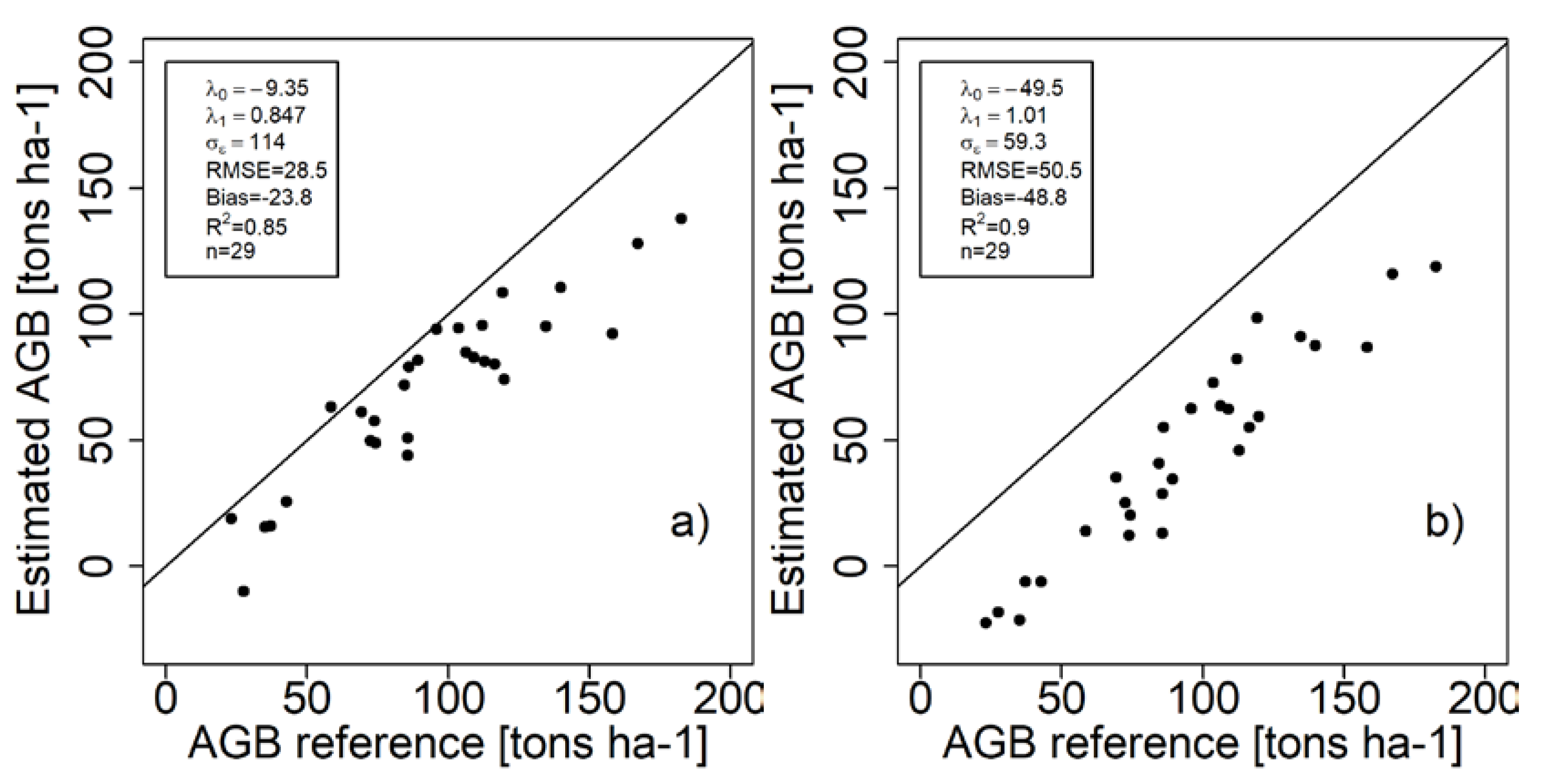
Sensor	Dataset	${\mathit{\lambda }}_0^{*}$	${\mathit{\lambda }}_1^{*}$	${\mathit{\sigma }}_{\mathit{\epsilon }}^2{}^{*}$	${\mathit{t}}_{\mathit{v}\mathit{a}\mathit{l}\mathit{u}\mathit{e}}^{*}$	q	RMSE tons/ha	RMSE* tons/ha
TanDEM-X	Krycklan	−9.35	0.847	114	−2.90	1.31	28.5	26.1
ALS	Krycklan	−49.5	1.01	59.3	−1.01	1.23	50.5	49.5

.

The corresponding scatterplots (predicted-vs-reference) are given in Figure 5a,b. Since the regression model indicates a systematic deviation for the evaluation test site, a few plots are predicted with negative biomasses. These have no physical meaning and could be removed or truncated to zero. Merely investigating the RMSE values gives no explanation to why the ALS estimates appear worse than the TanDEM-X based estimates. However, scatterplots and visualizations of the error model reveal how the significant systematic deviation due to the ALS model causes the larger RMSE.

The estimated error model parameters may be displayed visually to simplify the understanding of how the error changes with the true AGB (Figure 6). The figure shows the systematic errors for different true AGB values, and around the systematic error a $\pm 2{\widehat{\sigma }}_{\epsilon }$ wide band for the random error terms is displayed. For low AGB values, the error is smaller with the estimates based on TanDEM-X data, while at higher AGB values the errors approach similar magnitudes, although with different trends. The error related to the ALS estimates are however nearly constant for the entire range of values, but the downward shift is due to a bias. The t-values should be interpreted with regard to 27 degrees of freedom (29 stands – 2 parameters), where the tabulated two-tailed 95% t-value = 2.052. Hence, for the TanDEM-X based estimates the t-value −2.90 implies that the null hypothesis should be rejected. For the ALS case, where the t-value is −1.01, the null-hypothesis cannot be rejected and ${\lambda }_1$ may be considered as equal to one in the analysis. Hence, the special case (${\lambda }_1=1$) could have been used instead of computing both lambda parameters. Note that in Figure 5, the errors in the reference dataset complicates the visual interpretation, whereas in Figure 6 the effect of such errors have been removed.

In the dataset from Krycklan, the random errors in the field references were relatively small because of an ambitious study design where a large number of sample plots were distributed in each stand. Thus, the corrections due to random errors in the field references were fairly moderate in the case study demonstration. To illustrate the effects of larger random errors in the field reference, Figure 7 shows corrected and uncorrected estimates of RMSE for the case where additional random errors in the field reference data were added through simulation (1000 repetitions with error terms assumed to be normally distributed). When the random errors became very large, the correction exceeded the actual biomass and the corrected result would be a negative biomass, which can never appear in practice. These were therefore truncated to zero, which caused the small downward trend.

In the case study dataset, the standard deviation of errors in the field reference was about 10 tons/ha; it can be seen in Figure 7 that this magnitude of uncertainty in reference data has only a minor effect on the reported RMSEs. However, larger standard errors in the field reference would have led to substantial overestimation of the RMSE, unless the corrections proposed in this paper would not have been applied.

4. Discussion and Conclusions

This paper discusses the challenge of unambiguously reporting uncertainties when RS-based estimates of forest characteristics are computed and evaluated at the level of plots and stands by comparing them with field reference data. We demonstrate that conventional metrics such as RMSE or R2 are ambiguous and that clearly different error structures in the RS-based estimates may produce the same numerical values of these metrics. As an alternative, we propose that the parameters of a parametric error model should be estimated and presented. The error model is linear and consists of three parameters: ${\lambda }_0,{\lambda }_1$ and ${\sigma }_{\epsilon }^{}$, allowing for a wide range of error structures (e.g., see Figure 1, Figure 2, Figure 3 and Figure 5). The approach might be further developed by allowing for additional parameters offering more flexibility, such as heterogeneous random errors (a variable magnitude of the random errors across the range of true VOI values). Tian et al. [8,71] reported one such possibility, where logarithmic transformations make multiplicative errors additive. Yet, while the model (Equation (5)) is fairly simple it resolves several problems of under-determination, i.e., that different error structures can produce the same value of an uncertainty metric, by clearly separating systematic and random error components. Vasquez and Whiting [72] discussed how random and systematic errors could be accounted for in uncertainty propagations in computer models. This required additional Monte Carlo simulations and error propagation using Taylor’s series expansion, which increase the complexity. The error model we adapt is straightforward and generic, which facilitates comparisons, yet it is sufficiently complete to cover a wide range of different error structures. The parametric form makes it comprehensive, since the error for any true value can be computed, compared to conventional uncertainty metrics, where RMSE, bias and R² all have limitations. The parametric error model offers a possibility for standardized reporting of error structures and allows for adequate comparisons between different studies. However, since conventional metrics are difficult to ignore, methods for relating the proposed error parameters to bias and RMSE were also described. Inspection of density curves can also provide additional insight to the structure of uncertainties.

Our second objective was to extend the use of the parametric error model to cover cases where the field references used for evaluation contain random errors. The proposed estimators adjust for such random errors. It was further shown how they could be combined with the error model to evaluate the RS based estimates relative to the unobserved truth, and thus correct for uncertainties due to random reference errors. For the case of constant bias across the range of true values, we identified a special case where the variance of the random errors in the reference data should be subtracted from the traditional MSE estimator to obtain a corrected, unbiased, MSE* estimator. An adjusted Student’s t-test that corrects for regression dilution due to random errors in the reference data can be used to determine if the special case is applicable.

The error model parameters can be visualized as linear error bands vs. the reference values to provide an intuitive understanding of how the errors change across the range of true values. The band center represents the systematic error component and the width the random error component, for any true reference value (Figure 6). A potential development of this approach would be to allow for heteroscedastic errors in the error model.

The difference between the parametric error model adapted in this study and prediction models linking RS data with field references should be stressed. As described in the introduction, prediction models where the field reference is used as the dependent variable and the RS metrics as the independent variables, are often developed based on regression analysis [6,26,73,74,75]. Such models normally predict the field reference unbiasedly, conditional on the RS data. However, this does not mean that the model provides unbiased predictions conditional on the true field reference values. Instead, RS-based models often provide predictions that tend towards the mean, i.e., low true values are overestimated and high true values are underestimated [76]. With the error model, which links observed values with true values for the VOI, this is reflected through ${\lambda }_1$-values smaller than one. Thus, the residual variance from a prediction model (which is typically reported in RS studies) would not be equal to the residual variance of the error model, although the sizes would normally be of similar magnitude (e.g., [34]).

Corrections for errors in the reference data should be considered at least with q-values approaching 2 or lower. Depending on the application, this value might be chosen differently. Some papers using RS to generate digital elevation models suggest that the reference data should be at least three times better (q = 3) than the method to be evaluated [77,78]. From Figure 4, that corresponds to an overestimation of the RMSE with 5.4% and might hence be a reasonable rule of thumb.

Our discussion does not address the reasons for errors in field reference data and in the case study demonstration, it was assumed that sampling errors was the dominating random error source. This is normally the case for estimates at the stand level and it agrees with the error budget presented by [79]. Estimates at plot level may instead be limited by random positioning errors. These two error sources are expected to make up the absolutely dominating error part. This study assumed that the references were unbiased, hence not containing systematic errors. The magnitude and possible influence of, e.g., measurement errors and locational errors (crucial in RS) as random and systematic error components should be covered more in future studies. In addition, model errors (e.g., relating the inventoried diameter and tree species to biomass) were ignored in this study. The magnitude of model errors is likely to vary depending on the values of the input variables, and systematic model errors can sometimes contribute significantly to the total uncertainty [79].

The combination of presenting an error model and adjust for errors in the reference data has, to our knowledge, not been presented previously for RS-based forest applications. We adapt the proposed error model which agrees with the one presented by [8], and improve its use further. Problems related to regression dilution and uncertainties in the reference data in general have been discussed extensively in several books [12,13,14,66]. We propose a solution that covers both areas, which is relevant for many forest RS cases. We suggest that it could be used as a baseline for error reporting.

It is concluded that improved RS techniques make the reference data errors more important to consider (when compared to errors in RS-based estimates) and this paper provides a new method to quantify the effects of such errors and correct for them. We suggest that such corrections should be implemented if the ratio (q) between the standard deviation of random errors in the field reference and the standard deviation of random errors in the RS-based estimate is smaller than 2. By reporting the three parameters required for the error model, a more complete and transparent characterization of the errors in the RS-based estimates can be provided, which simplifies comparisons between studies.

References

- Tomppo, E.; Olsson, H.; Ståhl, G.; Nilsson, M.; Hagner, O.; Katila, M. Combining national forest inventory field plots and remote sensing data for forest databases. Remote Sens. Environ. 2008, 112, 1982–1999. [Google Scholar] [CrossRef]
- Næsset, E.; Gobakken, T. Estimation of above- and below-ground biomass across regions of the boreal forest zone using airborne laser. Remote Sens. Environ. 2008, 112, 3079–3090. [Google Scholar] [CrossRef]
- Mauya, E.W.; Hansen, E.H.; Gobakken, T.; Bollandsås, O.M.; Malimbwi, R.E.; Næsset, E. Effects of field plot size on prediction accuracy of aboveground biomass in airborne laser scanning-assisted inventories in tropical rain forests of Tanzania. Carbon Balance Manag. 2015, 10, 10. [Google Scholar] [CrossRef] [PubMed]
- Næsset, E. Accuracy of forest inventory using airborne laser scanning: Evaluating the first nordic full-scale operational project. Scand. J. For. Res. 2004, 19, 554–557. [Google Scholar] [CrossRef]
- Persson, H.; Fransson, J.E.S. Forest Variable Estimation Using Radargrammetric Processing of TerraSAR-X Images in Boreal Forests. Remote Sens. 2014, 6, 2084–2107. [Google Scholar] [CrossRef]
- Persson, H.J.; Fransson, J.E.S. Comparison between TanDEM-X and ALS based estimation of above ground biomass and tree height in boreal forests. Scand. J. For. Res. 2017, 32, 306–319. [Google Scholar] [CrossRef]
- Varvia, P. Uncertainty Quantification in Remote Sensing of Forests; University of Eastern Finland: Joensuu, Finland, 2018. [Google Scholar]
- Tian, Y.; Nearing, G.S.; Peters-Lidard, C.D.; Harrison, K.W.; Tang, L. Performance Metrics, Error Modeling, and Uncertainty Quantification. Mon. Weather Rev. 2016, 144, 607–613. [Google Scholar] [CrossRef]
- Pearson, K. On the Mathematical Theory of Errors of Judgment, with Special Reference to the Personal Equation. Philos. Trans. R. Soc. Lond. 1901, A198, 235–299. [Google Scholar]
- Wald, A. The Fitting of Straight Lines if Both Variables are Subject to Error. Ann. Math. Stat. 1940, 11, 284–300. [Google Scholar] [CrossRef]
- Gustafsson, P. Measurement Error and Misclassification in Statistics and Epidemiology: Impacts and Bayesian Adjustments, 1st ed.; Chapman & Hall/CRC: London, UK, 2004. [Google Scholar]
- Carroll, R.J.; Ruppert, D.; Stefanski, L.A.; Crainiceanu, C. Measurement Error in Nonlinear Models: A Modern Perspective, 2nd ed.; Chapman and Hall: Boca Raton, FL, USA, 2006. [Google Scholar]
- Buonaccorsi, J.P. Measurement Error Models, Methods and Applications; CRC Press: Boca Raton, FL, USA, 2010. [Google Scholar]
- Yi, G.Y. Statistical Analysis with Measurement Error or Misclassification: Strategy, Method and Application, 1st ed.; Springer Science+Business Media: New York, NY, USA, 2017. [Google Scholar]
- Marklund, L.G. Biomassafunktioner för Tall, Gran Och Björk i Sverige; Swedish University of Agricultural Sciences: Umeå, Sweden, 1988. [Google Scholar]
- Marklund, L.G. Biomass Functions for Norway Spruce (Picea Abies (L.) Karst.) in Sweden; Swedish University of Agricultural Sciences: Umeå, Sweden, 1987. [Google Scholar]
- Brandel, G. Volymfunktioner för Enskilda Träd: Tall, Gran Och Björk = Volume Functions for Individual Trees: Scots Pine (Pinus Sylvestris), Norway Spruce (Picea Abies) and Birch (Betula Pendula & Betula Pubescens); Swedish University of Agricultural Sciences: Garpenberg, Sweden, 1990; ISBN 9157640300 9789157640307. [Google Scholar]
- Nickless, A.; Scholes, R.J.; Archibald, S. A method for calculating the variance and confidence intervals for tree biomass estimates obtained from allometric equations. S. Afr. J. Sci. 2011, 107, 1–10. [Google Scholar] [CrossRef]
- Wulder, M.; Franklin, S.E. Remote Sensing of Forest Environments: Concepts and Case Studies; Springer: New York, NY, USA, 2003. [Google Scholar]
- Saatchi, S.S.; Quegan, S.; Ho Tong Minh, D.; Le Toan, T.; Scipal, K.; Carreiras, J.M.B.; Carvalhais, N.; Reichstein, M. Coverage of high biomass forests by the ESA BIOMASS mission under defense restrictions. Remote Sens. Environ. 2017, 196, 154–162. [Google Scholar]
- Tansey, K.; Louis, V.; Wheeler, J.; Balzter, H.; Rodríguez-Veiga, P. Quantifying Forest Biomass Carbon Stocks From Space. Curr. For. Rep. 2017, 3, 1–18. [Google Scholar]
- Næsset, E. Airborne laser scanning as a method in operational forest inventory: Status of accuracy assessments accomplished in Scandinavia. Scand. J. For. Res. 2007, 22, 433–442. [Google Scholar] [CrossRef]
- Datla, R.V.; Kessel, R.; Smith, A.W.; Kacker, R.N.; Pollock, D.B. Uncertainty analysis of remote sensing optical sensor data: Guiding principles to achieve metrological consistency. Int. J. Remote Sens. 2010, 31, 867–880. [Google Scholar] [CrossRef]
- Varvia, P.; Lahivaara, T.; Maltamo, M.; Packalen, P.; Tokola, T.; Seppänen, A. Uncertainty Quantification in ALS-Based Species-Specific Growing Stock Volume Estimation. IEEE Trans. Geosci. Remote Sens. 2017, 55, 1671–1681. [Google Scholar] [CrossRef]
- Næsset, E. Predicting forest stand characteristics with airborne scanning laser using a practical two-stage procedure and field data. Remote Sens. Environ. 2002, 80, 88–99. [Google Scholar] [CrossRef]
- Hyyppä, J.; Kelle, O.; Lehikoinen, M.; Inkinen, M. A segmentation-based method to retrieve stem volume estimates from 3-D tree height models produced by laser scanners. IEEE Trans. Geosci. Remote Sens. 2001, 39, 969–975. [Google Scholar] [CrossRef]
- Pitkänen, J.; Maltamo, M. Adaptive Methods for Individual Tree Detection on Airborne Laser Based Canopy Height Model. Int. Arch. 2004, 36, 187–191. [Google Scholar]
- Dalponte, M.; Bruzzone, L.; Gianelle, D. A system for the estimation of single-tree stem diameter and volume using multireturn LIDAR data. IEEE Trans. Geosci. Remote Sens. 2011, 49, 2479–2490. [Google Scholar] [CrossRef]
- Dalponte, M.; Ørka, H.O.; Ene, L.T.; Gobakken, T.; Næsset, E. Tree crown delineation and tree species classification in boreal forests using hyperspectral and ALS data. Remote Sens. Environ. 2014, 140, 306–317. [Google Scholar] [CrossRef]
- Fridman, J.; Holm, S.; Nilsson, M.; Nilsson, P. Adapting National Forest Inventories to changing requirements–the case of the Swedish National Forest Inventory at the turn of the 20th century. Silva Fenn. 2014, 48, 1–29. [Google Scholar] [CrossRef]
- Eid, T.; Næsset, E. Determination of stand volume in practical forest inventories based on field measurements and photo-interpretation: The Norwegian experience. Scand. J. For. Res. 1998, 13, 246–254. [Google Scholar] [CrossRef]
- Strand, L. Determination of Volume by Means of the Relascope. For. Sci. 1964, 10, 1964. [Google Scholar]
- Henttonen, H.M.; Kangas, A. Optimal plot design in a multipurpose forest inventory. For. Ecosyst. 2015, 2, 31. [Google Scholar] [CrossRef]
- Ståhl, G. A Study on the Quality of Compartmentwise Forest Data Acquired by Subjective Inventory Methods; Swedish University of Agricultural Sciences: Umeå, Sweden, 1992; Volume 24. [Google Scholar]
- Gregoire, T.G.; Valentine, H.T. Sampling Strategies for Natural Resources and the Environment; Chapman and Hall: Boca Raton, FL, USA, 2008; Volume 64. [Google Scholar]
- Saarela, S.; Schnell, S.; Tuominen, S.; Balázs, A.; Hyyppä, J.; Grafström, A.; Ståhl, G. Effects of positional errors in model-assisted and model-based estimation of growing stock volume. Remote Sens. Environ. 2016, 172, 101–108. [Google Scholar] [CrossRef]
- McRoberts, R.E.; Chen, Q.; Walters, B.F.; Kaisershot, D.J. The effects of global positioning system receiver accuracy on airborne laser scanning-assisted estimates of aboveground biomass. Remote Sens. Environ. 2018, 207, 42–49. [Google Scholar] [CrossRef]
- Gobakken, T.; Næsset, E. Assessing effects of positioning errors and sample plot size on biophysical stand properties derived from airborne laser scanner data. Can. J. For. Res. 2009, 39, 1036–1052. [Google Scholar] [CrossRef]
- Mauro, F.; Valbuena, R.; Manzanera, J.A. Influence of Global Navigation Satellite System errors in positioning inventory plots for tree- height distribution studies 1. Can. J. For. Res. 2011, 23, 11–23. [Google Scholar] [CrossRef]
- Frazer, G.W.; Magnussen, S.; Wulder, M.A.; Niemann, K.O. Simulated impact of sample plot size and co-registration error on the accuracy and uncertainty of LiDAR-derived estimates of forest stand biomass. Remote Sens. Environ. 2011, 115, 636–649. [Google Scholar] [CrossRef]
- Saarela, S.; Holm, S.; Healey, S.P.; Andersen, H.-E.; Petersson, H.; Prentius, W.; Patterson, P.L.; Naesset, E.; Gregoire, T.G.; Ståhl, G. Generalized Hierarchical Model-Based Estimation for Aboveground Biomass Assessment Using GEDI and Landsat Data. Remote Sens. 2018, 10, 1832. [Google Scholar] [CrossRef]
- Campbell, J.B. Introduction to Remote Sensing, 4th ed.; The Builford Press: New York, NY, USA, 2007. [Google Scholar]
- Barnston, A.G. Correspondence among the Correlation, RMSE, and Heidke Forecast Verification Measures; Refinement of the Heidke Score. Weather Forecast. 1992, 7, 699–709. [Google Scholar] [CrossRef]
- Barnston, A.G.; Thomas, J.L. Rainfall Measurement Accuracy in FACE: A Comparison of Gage and Radar Rainfalls. J. Clim. Appl. Meterol. 1983, 22, 2038–2052. [Google Scholar] [CrossRef]
- Yin, P.; Fan, X. Estimating r2 shrinkage in multiple regression: A comparison of different analytical methods. J. Exp. Educ. 2001, 69, 203–224. [Google Scholar] [CrossRef]
- Cramer, J.S. Mean and variance of R2 in small and moderate samples. J. Econ. 1987, 35, 253–266. [Google Scholar] [CrossRef]
- Mukaka, M.M. Statistics corner: A guide to appropriate use of correlation coefficient in medical research. Malawi Med. J. 2012, 24, 69–71. [Google Scholar] [PubMed]
- Hendry, D.F.; Marshall, R.C. On High and Low R2 Contributions. Oxf. Bull. Econ. Stat. 1983, 45, 313–316. [Google Scholar] [CrossRef]
- Moraes, D. Letters The Coefficient of Determination: What. Investig. Ophtalmol. Vis. Sci. 2012, 53, 6830–6832. [Google Scholar]
- Marcot, B.G. Metrics for evaluating performance and uncertainty of Bayesian network models. Ecol. Modell. 2012, 230, 50–62. [Google Scholar] [CrossRef]
- Valbuena, R.; Hernando, A.; Manzanera, J.A.; Görgens, E.B.; Almeida, D.R.A.; Mauro, F.; García-Abril, A.; Coomes, D.A. Enhancing of accuracy assessment for forest above-ground biomass estimates obtained from remote sensing via hypothesis testing and overfitting evaluation. Ecol. Modell. 2017, 366, 15–26. [Google Scholar] [CrossRef]
- Papoulis, A. Probability, Random Variables and Stochastic Processes, 2nd ed.; McGraw-Hill Education: New York, USA, 1984. [Google Scholar]
- Wilks, D. Statistical Methods in the Atmospheric Sciences, 3rd ed.; Academic Press: Cambridge, MA, USA, 2011; ISBN 9780123850225. [Google Scholar]
- Fonseca, J.R.; Friswell, M.I.; Mottershead, J.E.; Lees, A.W. Uncertainty identification by the maximum likelihood method. J. Sound Vib. 2005, 288, 587–599. [Google Scholar] [CrossRef]
- Livezey, R.E.; Hoopingarner, J.D. Verification of Official Monthly Mean 700-hPa Height Forecasts: An Update. Weather Forecast. 1995, 10, 512–527. [Google Scholar] [CrossRef][Green Version]
- Murphy, A.H. The Coefficients of Correlation and Determination as Measures of performance in Forecast Verification. Weather Forecast. 1995, 10, 681–688. [Google Scholar] [CrossRef]
- Reese, H.; Nilsson, M.; Pahlén, T.; Pahén, T.; Hagner, O.; Joyce, S.; Tingelöf, U.; Egberth, M.; Olsson, H.; Pahlén, T. Countrywide estimates of forest variables using satellite data and field data from the National Forest Inventory. AMBIO A J. Hum. Environ. 2003, 32, 542–548. [Google Scholar] [CrossRef] [PubMed]
- Lu, D. Aboveground biomass estimation using Landsat TM data in the Brazilian Amazon. Int. J. Remote Sens. 2005, 26, 2509–2525. [Google Scholar] [CrossRef]
- Labrecque, S.; Fournier, R.A.; Luther, J.E.; Piercey, D. A comparison of four methods to map biomass from Landsat-TM and inventory data in western Newfoundland. For. Ecol. Manag. 2006, 226, 129–144. [Google Scholar] [CrossRef]
- Askne, J.I.H.; Fransson, J.E.S.; Santoro, M.; Soja, M.J.; Ulander, L.M.H. Model-based biomass estimation of a hemi-boreal forest from multitemporal TanDEM-X acquisitions. Remote Sens. 2013, 5, 5574–5597. [Google Scholar] [CrossRef]
- Mitchard, E.T.A.; Saatchi, S.S.; Woodhouse, I.H.; Nangendo, G.; Ribeiro, N.S.; Williams, M.; Ryan, C.M.; Lewis, S.L.; Feldpausch, T.R.; Meir, P. Using satellite radar backscatter to predict above-ground woody biomass: A consistent relationship across four different African landscapes. Geophys. Res. Lett. 2009, 36, L23401. [Google Scholar] [CrossRef]
- Persson, H.J.; Olsson, H.; Soja, M.J.; Ulander, L.M.H.; Fransson, J.E.S. Experiences from large-scale forest mapping of Sweden using TanDEM-X data. Remote Sens. 2017, 9, 1253. [Google Scholar] [CrossRef]
- Fransson, J.E.S.; Israelsson, H. Estimation of stem volume in boreal forests using ERS-1 C- and JERS-1 L-band SAR data. Int. J. Remote Sens. 1999, 20, 123–137. [Google Scholar] [CrossRef]
- Nilsson, M.; Nordkvist, K.; Jonzén, J.; Lindgren, N.; Axensten, P.; Wallerman, J.; Egberth, M.; Larsson, S.; Nilsson, L.; Eriksson, J.; et al. A nationwide forest attribute map of Sweden derived using airborne laser scanning data and field data from the national forest inventory. Remote Sens. Environ. 2017, 194, 447–454. [Google Scholar] [CrossRef]
- Yu, X.; Hyyppä, J.; Karjalainen, M.; Nurminen, K.; Karila, K.; Kukko, A.; Jaakkola, A.; Liang, X.; Wang, Y.; Hyyppä, H.; et al. Comparison of laser and stereo optical, SAR and InSAR point clouds from air- and space-borne sources in the retrieval of forest inventory attributes. Remote Sens. 2015, 7, 15933–15954. [Google Scholar] [CrossRef]
- Fuller, W.A. Measurement Error Models, 1st ed.; John Wiley & Sons: New York, NY, USA, 1987. [Google Scholar]
- Frost, C.; Thompson, S.G. Correcting for Regression Dilution Bias: Comparison of Methods for a Single Predictor Variable. J. R. Stat. Soc. Ser. A 2000, 163, 173–189. [Google Scholar] [CrossRef]
- Li, C. Mathematical Models in Forest Resource Management Planning. An Integrated Study of Calibration, Prediction and Optimal Decision Models; Report 18; Swedish University of Agricultural Sciences: Umeå, Sweden, 1988. [Google Scholar]
- Hutcheon, J.A.; Chiolero, A.; Hanley, J.A. Random measurement error and regression dilution bias. BMJ 2010, 340, c2289. [Google Scholar] [CrossRef]
- Mcinerny, G.J.; Purves, D.W. Fine-scale environmental variation in species distribution modelling: Regression dilution, latent variables and neighbourly advice. Methods Ecol. Evol. 2011, 2, 248–257. [Google Scholar] [CrossRef]
- Tian, Y.; Huffman, G.J.; Adler, R.F.; Tang, L.; Sapiano, M.; Maggioni, V.; Wu, H. Modeling errors in daily precipitation measurements: Additive or multiplicative? Geophys. Res. Lett. 2013, 40, 2060–2065. [Google Scholar] [CrossRef]
- Vasquez, V.R.; Whiting, W.B. Accounting for both random errors and systematic errors in uncertainty propagation analysis of computer models involving experimental measurements with Monte Carlo methods. Risk Anal. 2006, 25, 1669–1681. [Google Scholar] [CrossRef]
- Solberg, S.; Astrup, R.; Gobakken, T.; Næsset, E.; Weydahl, D.J. Estimating spruce and pine biomass with interferometric X-band SAR. Remote Sens. Environ. 2010, 114, 2353–2360. [Google Scholar] [CrossRef]
- Nilsson, M. Estimation of tree heights and stand volume using an airborne lidar system. Remote Sens. Environ. 1996, 56, 1–7. [Google Scholar] [CrossRef]
- Næsset, E.; Gobakken, T.; Holmgren, J.; Hyyppä, H.; Hyyppä, J.; Maltamo, M.; Nilsson, M.; Olsson, H.; Persson, Å.; Söderman, U.; et al. Laser scanning of forest resources: The nordic experience. Scand. J. For. Res. 2004, 19, 482–499. [Google Scholar] [CrossRef]
- Nilsson, M. Estimation of Forest Variables Using Satellite Image Data and Airborne Lidar. Ph.D. Thesis, Swedish University of Agricultural Sciences, Umeå, Sweden, 1997. [Google Scholar]
- Höhle, J.; Höhle, M. Accuracy assessment of digital elevation models by means of robust statistical methods. ISPRS J. Photogramm. Remote Sens. 2009, 64, 398–406. [Google Scholar] [CrossRef]
- Maune, D.F. Digital Elevation Model Technologies and Applications: The DEM User Manual, 2nd ed.; American Society for Photogrammetry and Remote Sensing (ASPRS): Bethesda, MD, USA, 2007; ISBN 1-57083-082-7. [Google Scholar]
- Gertner, G.Z.; Köhl, M. An Assessment of Some Nonsampling Errors in a National Survey Using an Error Budget. For. Sci. 1992, 38, 525–538. [Google Scholar]