Abstract
Surpervoxels are becoming increasingly popular in many point cloud processing applications. However, few methods have been devised specifically for generating compact supervoxels from unstructured three-dimensional (3D) point clouds. In this study, we aimed to generate high quality over-segmentation of point clouds. We propose a merge-swap optimization framework that solves any supervoxel generation problem formulated in energy minimization. In particular, we tailored an energy function that explicitly encourages regular and compact supervoxels with adaptive size control considering local geometric information of point clouds. We also provide two acceleration techniques to reduce the computational overhead. The performance of the proposed merge-swap optimization approach is superior to that of previous work in terms of thorough optimization, computational efficiency, and practical applicability to incorporating control of other properties of supervoxels. The experiments show that our approach produces supervoxels with better segmentation quality than two state-of-the-art methods on three public datasets.
1. Introduction
Segmentation of a point cloud is a coarse partition at the object level, whereas over-segmentation is much finer. Surpervoxels provide over-segmentation of a point cloud. As they provide a more compact and perceptually meaningful representation than the original point cloud, supervoxels are beneficial for many applications in point cloud processing, such as semantic labelling [1], classification [2], saliency detection [3], and object detection [4]. The term of supervoxel is also used in the context of video and three-dimensional (3D) medical image processing [5,6], where 3D grid pixels are grouped into perceptually meaningful regions conforming to object boundaries, extending the planar superpixels [7] to 3D space by clustering pixels in a stack of images. For point clouds produced by 3D laser scanners, supervoxels are defined as clusters of points with similar geometry or other low-level properties. Different from videos or RGB-Dimages, point clouds collected from 3D scanners are usually unorganized and include noise, outliers, and non-uniformities, which impose additional challenges on supervoxel generation.
Grouping points into small regions can significantly improve the efficiency of algorithms that rely upon point-based data structure, especially for processing large-scale point clouds. Hence, supervoxels have been widely used in broad applications ranging from remote sensing to computer vision and graphics. Hence, the pre-processing techniques for efficiently generating supervoxels from 3D points are increasing in importance. As a more natural representation of 3D point clouds, supervoxels need to exhibit the following traits:
- Adherence to boundaries: As supervoxels are commonly used as processing units to segment and detect objects, the most important property is adherence to object boundaries.
- Regular and compact shape patterns: Supervoxels should exhibit regular and compact shape patterns in regions without boundaries or features, as they will produce a simpler adjacency graph for later processing.
- Size adaptive to local contents: To reduce the complexity of a point cloud, the size of supervoxels should be adaptive to local contents of a point cloud, i.e., larger supervoxels are in plain regions whereas smaller supervoxels are in complex regions.
The two-dimensional (2D) counterpart of supervoxel segmentation is superpixel segmentation, which was found to be a useful preprocessing step in many computer vision tasks and has received considerable attention. A variety of superpixel segmentation methods have been proposed over the past few years. In stark contrast, oversegmenting point clouds into supervoxels has received far less attention. This is perhaps due to 3D point clouds being larger and more complex than a 2D image. Extending a superpixel generation method to 3D point clouds is complex, as existing superpixel methods heavily rely upon the intrinsic neighboring relationships between pixels and it is theoretically impossible to convert an unorganized into an organized point cloud. Hence, generating supervoxels from 3D point clouds is challenging.
Few methods have been devised specifically for supervoxel generation. Voxel cloud connectivity segmentation (VCCS) [8] was an early supervoxel method that generates over-segmentation from 3D point clouds. The space is first divided into a voxelized grid with a given resolution, and then a number of seed points are selected from the voxelized space to initialize the supervoxels. Other points are assigned to supervoxels using a local k-means clustering method [7]. VCCS generates uniform supervoxels without considering local features and geometric complexities of a scene. A recent method better boundary preserved supervoxel segmentation (BPSS) ([9]) formalizes supervoxel segmentation as a subset selection problem and uses a heuristic method to minimize the objective function. Approximate solutions from the BPSS method may lead to supervoxels violating object boundaries.
In this study, we focused on generating supervoxels from 3D point clouds. We developed a variational approach to generate supervoxels with the aforementioned desirable properties. Our specific contributions are as follows:
- We develop a supervoxel generation framework that solves an energy optimization problem with a target supervoxel number. The proposed framework is composed of two major components: merging and swapping. In the merging stage, small supervoxels are greedily merged into big ones if this operation minimizes the energy increase. The merging process continues until the number of supervoxels reaches a preset value. Then in the swapping stage, points located at supervoxel boundaries are swapped if the total energy of their two adjacent supervoxels decreases. The swapping is repeatedly performed until no further decrease in energy is possible.
- We propose two acceleration techniques for processing large-scale point clouds: the adaptive octree and the three-level heap. The former generates fine supervoxels according to normal information, which serves as the input of the merging operation. The latter builds a min-heap in a divide-and-conquer manner to store the merging pair with globally minimal cost.
- We propose an energy function that combines three main desirable properties of the supervoxels: (1) planarity and normal similarity of points in supervoxels, (2) adherence to object boundaries, and (3) compact shape patterns. This energy function can be minimized using the proposed framework. The presented variational approach provides the flexibility to incorporate the control of other properties of supervoxels, such as color similarity.
The remainder of this paper is organized as follows. After providing a brief review of superpixel and supervoxel generation methods in Section 2, we introduce the merge-swap framework in detail in Section 3.1. With the definition of a new energy function for supervoxels, we explain how to apply the proposed optimization framework to generate supervoxels in Section 3.2. Two acceleration techniques are introduced in Section 4. The experimental results and comparisons are outlined in Section 5. Finally, we conclude this paper with an overall discussion that includes the implications of our findings, the limitations of our research, and future directions in Section 6.
2. Related Work
In contrast to superpixel generation in 2D image processing, less research on supervoxel generation for 3D point clouds has been published. In this section, we briefly review references most related to our work.
2.1. Superpixel Generation from RGB-D Images
Many superpixel approaches have been proposed in recent years [10,11,12]. Stutz et al. [13] presented a comprehensive evaluation of 28 state-of-the-art superpixel algorithms, and some of them were designed for or can be extended to processing RGB-D images [11,14,15,16,17,18]. With given depth information, an RGB-D image can be viewed as a 3D point set with given neighboring relationships in the camera coordinate system. Depth information can be combined with the colors to measure similarity between superpixels. For instance, the depth-adaptive superpixel method [14] extends simple linear iterative clustering (SLIC) [7] to a nine-dimensional feature space composed of colors, 3D coordinates, and normals. Yang et al. [19] proposed a similar method in which the distance from a cluster center to a pixel depends on the differences of CIELABcolors, depths, and 2D pixel locations. Different from these two methods, in the approach proposed by [16], the neighboring relationship between pixels is used to firstly generate a triangular mesh by triangulating pixels. Then, the triangular mesh is over-segmented into small regions using a defined weighted geodesic metric.
All these existing superpixel methods heavily rely on the regular structure of pixels and cannot be directly applied to supervoxel segmentation of unorganized 3D point clouds. The proposed merge-swap framework for supervoxel generation was inspired by the optimization technique proposed by [20], which was used to efficiently build superpixels by [11,21]. Equipped with a tailored energy function for supervoxels and adapted merging and swapping operations for point clouds, the proposed method generates compact supervoxels that adhere well to object boundaries.
2.2. Supervoxel Generation from 3D Point Clouds
To the best of our knowledge, only a few existing methods focus on supervoxel generation from 3D point clouds. The VCCS method [8] was the first to consider supervoxel segmentation of 3D point clouds. The input cloud is voxelized using an octree with fixed voxel resolution, and then seed points are placed by uniformly partitioning the 3D space with the seed resolution controlling the size of supervoxels. Supervoxels are initially selected as voxels containing seed points and then neighboring voxels are iteratively absorbed. Despite the efficiency of the VCCS method, it may fail when processing point clouds with non-uniform density, as some initial voxels may cover more than one object. Seed point selection influences the final segmentation, and boundaries of small objects are difficult to capture if they are missed by seed points.
Song et al. [22] proposed a supervoxel algorithm for sparse outdoor LiDARdata, which needs to detect the boundary points first. It first constructs a neighborhood graph by connecting neighboring points and removing boundary points, and then generates supervoxels by expanding cluster regions on the neighborhood graph and assigning boundary points to the closest cluster. This algorithm strongly depends on the boundary detection results and does not work well for complex data with noise and outliers. Kim and Park [23] improved it by introducing a weighted neighborhood graph. Seed points of clusters are selected and then expanded to other points by computing the shortest distance on the weighted graph. The over-segmentation results of this method are affected by the selection of the initial seed points.
Ref. [9] formulated supervoxel generation as a subset selection problem. Since the subset selection problem is NP-hard, they proposed a heuristic optimization method to minimize the energy function. The optimization framework includes fusion and exchange operations, both of which provide an approximate solution to the original subset selection problem. Due to the sub-optimal results obtained from the optimization method, some supervoxels may across object boundaries.
Compared with the original points, supervoxels provide a highly approximated representation with much less data, which helps accelerate the downstream applications, such as segmentation and classification [24].
3. Methodology
3.1. Merge-Swap Framework
In this section, we propose a simple merge-swap framework to generate supervoxels from 3D point clouds. For a given point set with n points, we set each point to be a supervoxel at the beginning. For each supervoxel , we define an energy term that measures the dissimilarity between points within a supervoxel. Then, we obtain the total energy function:
We provide a detailed definition of the energy function in Section 3.2.1. We aimed to reduce the total number of supervoxels to a user specified value K while minimizing the increase in the total energy. To achieve that, we propose a bottom-up optimization method. Starting from the input point set, the proposed method first generates supervoxels by iteratively merging supervoxel pairs with the minimal cost of energy. Then, it applies the point swapping operation to neighboring supervoxels to further decrease the energy function. We describe the details of the merging and swapping operations in Section 3.1.1 and Section 3.1.2, respectively.
3.1.1. Merging
Merging is an operation that groups two supervoxels into one, denoted by . As mentioned previously, our task was to obtain K supervoxels with minimal energy . The initial energy for the input data is . Merging two supervoxels into one generally results in increased energy. Our strategy was to iteratively choose a supervoxel pair with the slightest energy increase after merging.
For merging and , we define the merging cost as:
which is the increased energy after grouping the original points in and together. In each iteration, we evaluate all candidate supervoxel pairs and choose the one with the minimal merging cost. A min-heap is used to sort supervoxel pairs and find the minimum.
Note that we only consider neighboring supervoxels for merging for the sake of compactness. Thus, for a given point cloud, we organize the points using a k-d tree to facilitate the nearest neighbor searches. For each point, we find its M nearest neighbors and save this connection information in a neighboring graph . In our experiments, we set M to 20 by default. A supervoxel is considered a neighbor of a supervoxel if any points of and are adjacent in the neighboring graph . We initialized the min-heap by inserting all neighboring pairs. In practice, we only consider neighboring supervoxel pairs with to avoid duplication of supervoxel pairs in the min-heap. The merging stage stops when the supervoxel number is reduced to the user-specified number K. The pseudo-code of the merging process is provided in Algorithm 1.
| Algorithm 1 Merging | |
| Input: Point cloud with n points, and target supervoxel number K | |
| Output:K supervoxels | |
| 1: | compute neighboring graph ; |
| 2: | ; |
| 3: | declare an empty minimum heap H sorted by merging cost; |
| 4: | for each do |
| 5: | find its neighboring supervoxels and insert the pairs into H; |
| 6: | end for |
| 7: | repeat |
| 8: | pop the top element of H; |
| 9: | if both and are valid then |
| 10: | ; |
| 11: | invalidate and ; |
| 12: | find neighbors of and insert the pairs into H; |
| 13: | end if |
| 14: | until the number of supervoxels is equal to K |
3.1.2. Swapping
The merging operation can be regarded as a greedy method that groups small supervoxels into big ones. Once a supervoxel is formed, it will not be divided to obtain a better segmentation during the merging process. Here, we introduced the swapping operation, which is used to further refine the boundaries of supervoxels generated by the merging operation and leads to a lower value of the objective function.
For two neighboring supervoxels and , suppose that a point is moved from to , denoted by and . This point swapping is accepted if the energy function is reduced, i.e.,
To keep the supervoxels compact, we only consider boundary points for swapping. A point in a supervoxel is regarded as a boundary point if any of its adjacent points, denoted by , belongs to another supervoxel. A queue is used to store all boundary points. We iteratively test the front point in the queue to see if it can be swapped. After swapping a point i, we add i and its neighbors into the queue for further test if they are not in the queue. The swapping test continues until the queue is empty. See Algorithm 2 for more details about the swapping operation.
| Algorithm 2 Swapping | |
| Input: Point cloud , and K supervoxels. | |
| Output:K supervoxels with a lower energy. | |
| 1: | push the indices of boundary points of each supervoxel into a queue ; |
| 2: | repeat |
| 3: | pop the front element i from ; |
| 4: | get the supervoxel to which i belongs; |
| 5: | for each do |
| 6: | get the supervoxel that j belongs to; |
| 7: | if swap i from to is accepted then |
| 8: | , ; |
| 9: | ; |
| 10: | break out of for loop; |
| 11: | end if |
| 12: | end for |
| 13: | until is empty |
3.2. Supervoxel Generation
The proposed merge-swap optimization framework works for any energy function in the form of Equation (1). We will derive an energy function that is tailored for high-quality supervoxel generation in this section.
3.2.1. Energy Definition
Due to the energy driven property of the proposed framework, the energy function should be carefully designed so that neighboring points with similar properties can be merged into one supervoxel. According to the general requirements of a supervoxel representation, our energy definition for a supervoxel includes the coplanarity of points, normal similarity, and spatial regularity.
The position and normal are two basic attributes of a point; we denote them by and , respectively. The normals are either given by the user or estimated using the PCAmethod [25]. The differences in the average position and the average normal between supervoxels are usually used to measure the quality of an over-segmentation result [8,9]. In contrast, we focused on the differences in the position and normal of points in a supervoxel. For a supervoxel S, we first compute its average position and average unit normal , which determine a plane fitting to the supervoxel S. The fitting error is given by:
The above fitting energy describes the planarity of points in a supervoxel. However, the fitting energy cannot separate the points on the different sides of a sharp features well, since the distance from a point to the fitting plane on the other side of the sharp feature is generally small, as shown in Figure 1a. Note that the point normals change dramatically across the sharp feature. Thus, we introduced another energy term to measure the normal similarity of supervoxel S, which is defined as:
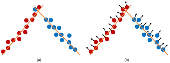
Figure 1.
Effect of the normal term: (a) clustering result by considering the fitting error only and (b) clustering result by considering both the fitting error and the normal similarity.
The dot product in the equation is squared to ignore its sign. Thus, the normals do not need to be consistently oriented over the entire point cloud.
Both the fitting term and the normal term account for the planarity of supervoxels and make the segmentation result conform to object boundaries (Figure 1b). However, for two neighboring supervoxels in a planar region, the boundary between them may be zigzag. To guarantee the compactness of supervoxels, we added another energy term on the supervoxels. It is defined as the summation of the squared distances from the center of a supervoxel to all its points:
This is a discrete version of the centroidal Voronoi tessellation energy [26], which is able to produce regular hexagonal patterns when minimized.
We formulated our total energy function for a supervoxel S as a weighted combination of the above three energy terms:
A proper selection of parameters produces feature preserving supervoxels with high regularity (Figure 1). We discuss the choice of these parameters in Section 3.2.3. The energy function defined in Equation (7) explicitly encourages regular and compact supervoxels with a size control adaptive to local geometric information of point clouds. It is also possible to incorporate the control of other properties of supervoxels in the same manner, such as color and intensity.
3.2.2. Fast Computation
The efficiency of computing the energy value for supervoxels after each merging or swapping operation is critical since it will be performed many times. A direct method is to traverse all the member points of a supervoxel and compute the accumulated energy value, which costs time, where n is the number of member points. We propose a method to compute the energy function. For each supervoxel S, we first define two matrices and :
Then, the above three energy items can be calculated using and , respectively. We have:
where is the point number of S.
We create a new supervoxel by merging a pair of neighboring supervoxels and . In the following, we evaluate the energy for . The average position of can be easily derived from the average positions of and . We have:
The average normal of can be obtained in the same manner. If we save the matrices and for each supervoxel , we can compute and following:
3.2.3. Weighting Parameters
The weighting factors and in our energy definition balance the importance of those three energy terms. A proper choice of weighting factors is crucial for the over-segmentation result. Theoretically, should be large enough to distinguish feature boundaries. As shown in the inset of Figure 2d, a large results in elongated supervoxels on the features. If is too small, boundaries are not preserved; see Figure 2c. In practice, an appropriate choice of highly depends on the input normals, as these normals are estimated and are generally inaccurate, especially for points near sharp features. Similarly, a larger implies that the supervoxels will be more regular and probably fail to preserve features of the point cloud; see Figure 2f. A small generates more zigzag boundaries; see the red circle in Figure 2e.
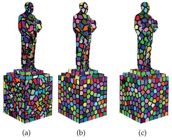
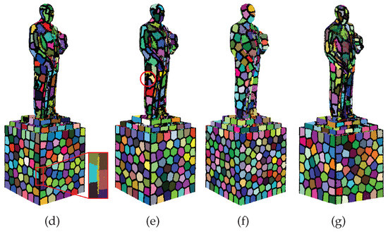
Figure 2.
Over-segmentation results (500 supervoxels) with different weighting parameters. Supervoxel boundaries are marked as black points. (a) Intermediate result after merging, ; (b) final over-segmentation result (after swapping) of (a); and (c–g) over-segmentation results with , , , , and , respectively.
We conducted a quantitative experiment on the point cloud, as shown in Figure 2, using different combinations of weighting parameters and as shown in Figure 3. We increased gradually from 0 to 0.1 and decreased gradually from 0.1 to 0. To quantitatively evaluate the results, we adopted three metrics: boundary recall, under-segmentation error, and global consistency error, which are introduced in Section 5.2.1. We also counted the average number of neighbors for each result to indicate the complexity of the adjacency graph. As shown in Figure 3, the larger the , the better the boundary recall. When varies in , the boundary recall shows no obvious change. The average number of neighbors increased with decreasing . The under-segmentation error and the global consistency error achieved their minimum values when and were around . Taken together, we set by default in experiments. The user can adjust and to obtain different results according to specific applications. The suggested range for and is
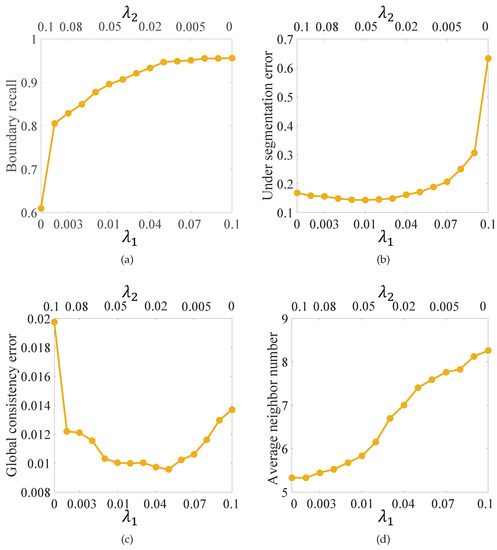
Figure 3.
Effects of different combinations of weighting parameters and . We set by default in experiments. (a) Boundary recall; (b) under segmentation error; (c) global consistency error; and (d) average neighbor number.
4. Implementation
In Section 3.2.2, we presented an efficient method for updating the energy function as required by every single merging and swapping operation. However, the proposed method still has heavy a computing burden in the merging stage when processing large-scale point clouds, as we need to dynamically maintain a large min-heap. Thus, in our implementation, we adopt two acceleration techniques to further speed up our method: three-level heaps and adaptive octree. The basic idea here is to reduce the size of the min-heap.
4.1. Three-Level Heaps
The first acceleration technique idivides the large heap into several small heaps. We adopt the following three-level structure to build a min-heap based on the concept of divide-and-conquer. As illustrated in Figure 4, the bottom level consists of min-heaps for each supervoxel. Every supervoxel has its own min-heap whose elements are the candidate merging pairs formed by its neighboring supervoxels and itself. In the middle level, we have h (=) min-heaps. The top element of a min-heap associated with the supervoxel k in the bottom level is inserted into a middle heap with the index of k mod h. The top level has only one min-heap, which organizes the heap index and the associated minimal cost of the middle heaps. Thus, we first collect merging pairs for each supervoxel and store them in the bottom-level heaps. All the top, elements of each bottom heap are then inserted into the middle heaps with corresponding indices. After that, we fill the top heap with the top elements of middle heaps.

Figure 4.
Illustration of three-level heaps. The bottom-level heap organizes merging pairs formed by a supervoxel and its neighbors, the middle-level heap organizes the top elements from the bottom-level heaps, and the top-level heap organizes the top elements from the middle-level heaps.
With these three-level heaps, the top element of the top heap yields the merging pair with the globally minimal cost, and we can find the indices of two merging supervoxels by traversing down the three-level min-heaps. The maximal size of the min-heap is reduced from n to , which notably reduces the computational load for maintaining min-heaps. Our experiments showed that it improves the efficiency of the optimization more than two-fold. As demonstrated in Figure 5, the three-level-heap acceleration technique effectively accelerates supervoxel generation.
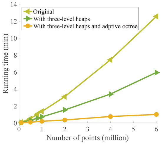
Figure 5.
Performance of our accelerating techniques. The three-level-heap acceleration technique improves the efficiency of the optimization significantly, and the adaptive-octree acceleration technique further improves the efficiency.
4.2. Adaptive Octree
An adaptive octree for point clouds consists of voxels with different sizes, where large voxels appear in smooth regions and small voxels appear at edges, corners, and in complex regions. This kind of octree is able to preserve object boundaries better than octrees with fixed voxel size, and it has been widely used in various applications to accelerate calculation, including ray tracing [27], point cloud segmentation [28], mesh generation [29,30,31,32], and finite element analysis [33,34].
For a given point cloud, the normal information is used to build an adaptive octree. Specifically, an octree is firstly constructed by subdividing the bounding box of the point cloud into uniform grids. Then, we check each grid to see if the maximum angle between normals of member points in the grid is greater than 60 degrees. If so, the grid is further subdivided. An example of an adaptive octree is shown in Figure 6. The adaptive octree actually clusters the points into fine voxels. The original points in Algorithm 1 are then replaced with voxels. That is, the merging operation starts with fine voxels instead of the original points of the input point cloud. This improves the convergence speed and reduces the calculation effort.
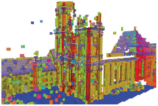
Figure 6.
An adaptive octree of a point cloud. Each octree node is color-coded by the average normal of its member points.
Adaptive octree-based merging is reasonable since points with similar normals are supposed to be grouped together. Even if some points are misclustered in the merging stage, the subsequent swapping operation will be able to rectify the problem. We provide a comparison in Figure 7, where supervoxels are generated with and without adaptive octree-based merging for a large-scale point cloud. Three quality measurements, which will be introduced later in Section 5.2.1, were computed to quantify the results. Adaptive octree-based merging had a negligible influence on the final supervoxel segmentation results. Thee speed advantages provided by the adaptive octree are substantial, as demonstrated in Figure 5. Benefiting from the proposed two acceleration techniques, the final merge-swap scheme is considerably faster than the original algorithm.

Figure 7.
The 10,000 supervoxels generated by our merge-swap method with and without adaptive octree-based merging, respectively, from 5.5 million input points. (a) The ground truth; (b) result with octree-based merging and , , , and running time = 80 s; and (c) result without octree-based merging and , , , and running time = 4.5 min.
5. Results and Discussion
In this section, we present several experimental results to demonstrate the effectiveness of our merge-swap method, and provide a comparison with the VCCS [8] and the BPSS methods [9]. The VCCS method was implemented using the Point Cloud Library (http://www.pointclouds.org) (PCL) and the BPSS method was performed using the authors’ implementation, which is publicly available online (https://github.com/yblin/Supervoxel-for-3D-point-clouds). All the experiments were performed on a laptop with an Intel Core i7 2.3GHz CPU and 16 GB RAM.
5.1. Supervoxel Segmentation Examples
Several examples in Figure 7, Figure 8, Figure 9 and Figure 10 demonstrate the efficacy of our method. In Figure 8, we compare the supervoxel results generated by the VCCS method, the BPSS method, and our merge-swap method. The two enlarged views show that our results conform better to object boundaries than the others. Our supervoxel segmentation provides a more natural representation of the ground, the wall, and the roof of the building. Larger supervoxels appear in planar regions, whereas smaller supervoxels appear in complex regions.
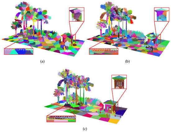
Figure 8.
The 357 supervoxels generated by (a) the VCCS method [8], (b) the BPSS method [9], and (c) our merge-swap method. Zoom-in views of the curb in each result are shown in the left-bottom corner. Points in different supervoxels are encoded using different colors.
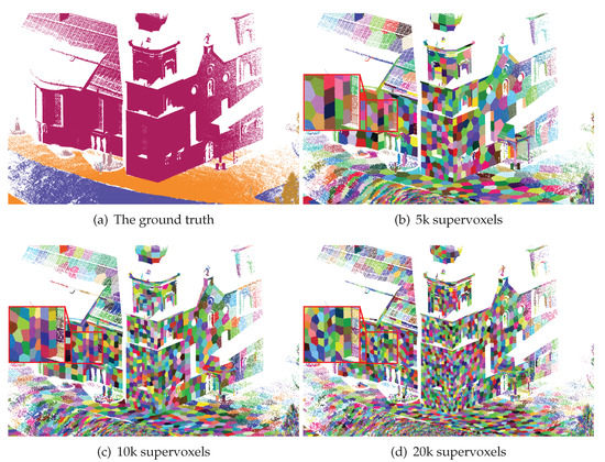
Figure 9.
Over-segmentation results with different numbers of supervoxels. (a)The ground truth; (b) 5000 supervoxels; , , ; (c) 10,000 supervoxels; , , ; and (d) 20,000 supervoxels; , , .
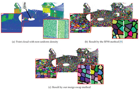
Figure 10.
Comparison on a point cloud with non-uniform density. Our merge-swap method generates supervoxels with varying resolution and more regular shapes than the BPSS method.
We ran the proposed method with different target numbers of supervoxels and computed the metric values, as shown in Figure 9. Generally, the larger the target number of supervoxels, the higher the boundary recall and the lower the segmentation error and the global consistency error. Note that the proposed method is able to obtain boundary preserved supervoxel segmentation even when the supervoxel number is small.
Our merge-swap method also works for point clouds with non-uniform density. One main merit of the BPSS method [9] is that it is capable of producing supervoxels with varying resolution according to the distribution of the points, so that smaller supervoxels appear in dense regions and larger supervoxels in sparse regions. Our merge-swap method is also able to distribute similar numbers of points in each supervoxel by equalizing the energy values of each supervoxel. Therefore, generating supervoxels with a non-fixed resolution is a built-in capability of our method. A comparison with the BPSS method on a non-uniform point cloud is shown in Figure 10. Supervoxels with varying resolution can be observed in the results of both methods. Nevertheless, our method obtains more regular supervoxels than the BPSS method.
5.2. Comparisons on Datasets
In this section, we compare our method with the VCCS [8] and BPSS [9] methods on three public datasets: NYU depth dataset V2 [35] (https://cs.nyu.edu/~silberman/datasets/nyu_depth_v2.html), Oakland [36] (http://www.cs.cmu.edu/~vmr/datasets/oakland_3d/cvpr09/doc/), and Semantic3D [37] (http://www.semantic3d.net/). Before demonstrating the comparison results, we briefly review three metrics used for measuring the quality of supervoxel segmentation.
5.2.1. Evaluation Metrics
We adopted three metrics, boundary recall (BR), ground truth error (UE), and global consistency error (GCE), which are natural extensions of metrics of superpixels in 2D image processing [7]. They have already been used in a supervoxel generation study [9]. To compute these values, a ground truth segmentation and a supervoxel segmentation should be provide. For completeness, we cite their definitions below:
Boundary recall (BR) is defined as the percentage of ground truth boundaries that are covered by supervoxel boundaries [38], and can be computed by:
where denotes ground truth boundaries and represents supervoxel boundaries. A point p is called a boundary if the label of one of its k-nearest neighbor points is different from that of p. A ground truth boundary point is covered if a supervoxel boundary point lies within the distance of to it. The same as [9], was set to m for indoor scene benchmarks and to m for outdoor scene benchmarks in our experiments.
Under-segmentation error (UE) is proposed for measuring the degree of supervoxels across the ground truth boundaries [39]. We compute it by:
where denote ground truth regions. For each ground truth region , we find all the supervoxels intersecting it, i.e., . Then, we count the number of points outside the region, and normalize it by the total point number n. A low under-segmentation error means that most supervoxels intersect with only one ground truth region and do not cross the ground truth boundaries.
Global consistency error (GCE) is another important metric that simultaneously evaluates under-segmentation both the over-segmentation error and the under-segmentation error [40]. Firstly, for a ground truth region and a supervoxel , we define the ground truth to supervoxel error as:
and the supervoxel to ground truth error as:
Then, we obtain the total number of intersecting points between the ground truth and supervoxels by:
GCE is defined as:
The value of GCE lies in , where 1 indicates the worst case and 0 corresponds to a perfect segmentation.
5.2.2. Performance on Datasets
For testing and comparison, we used the NYU depth V2 [35], Oakland [36] and Semantic3D [37] datasets, varying from indoor scenes to outdoor scenes. As each dataset contains point clouds with different sizes, we evaluated the three metrics on a dataset as the average of the corresponding metrics of all point clouds in that dataset. Comparisons were conducted by generating supervoxels on different scales. Note that the VCCS method cannot control the target number of the supervoxels precisely, as it generates uniformly distributed supervoxels. To enable a fair comparison, we first ran the VCCS method to generate supervoxels. Then, we specified the target number of the BPSS method and our merge-swap method to be the same as the number of supervoxels generated by the VCCS method. In other words, the segmentation results of three methods were compared against the same average size of supervoxels.
The NYU depth V2 dataset, which contains 1449 labeled RGB-D images, was adopted to test indoor scenes. The images were firstly converted to 3D point clouds, and each of them had up to 307,200 points. The metric curves of each method are shown in Figure 11. Our results show the best boundary recall and global consistency error for all average sizes of supervoxels, and our under-segmentation error curve is nearly the same as that of the BPSS method. This clearly demonstrates the better performance of the proposed approach on feature preserving against other existing methods. Note that point clouds converted from depth images usually contain sharp fluctuations. This highly non-coplanarity prevents all the compared methods from obtaining segmentation accurately conforming to the ground truth, hence leading to high UEs.
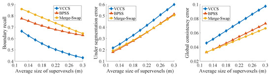
Figure 11.
Experimental results on NYU RGBD V2 dataset. Our merge-swap method achieved the highest BR and the lowest GCE, and a comparable UE to the BPSS method.
Both Oakland and Semantic3D consist of dense point clouds acquired from outdoor scenes. Oakland contains 17 clouds with sparse point density, which are labeled as 44 classes. The Semantic3D dataset consists of dense 3D point clouds with up to 4 billion points. The proposed approach typically needs 6GB memory to handle 10 million points. Limited by the memory size, we randomly down-sampled each cloud of Semantic3D to around 5 millions points. The comparisons of the three methods on these two datasets are shown in Figure 12 and Figure 13, respectively. The proposed method achieved the best performance in all three metrics for the Oakland dataset, and the highest boundary recall and the lowest global consistency error for the Semantic3D dataset.

Figure 12.
Experimental results on Oakland dataset. Our merge-swap method performed the best in all three metrics.
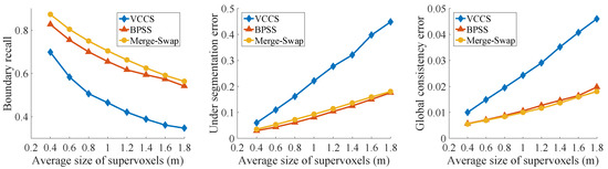
Figure 13.
Experimental results on the Semantic3D dataset. Our merge-swap method achieved the highest BR and the lowest GCE, and a UE close to that of the BPSS method.
5.3. Compactness Comparison
In 2D image processing, the compactness is another property that is desired for superpixel segmentation. The regularity or compactness of a superpixel was evaluated in [41]. Intuitively, a superpixel segmentation has higher compactness if superpixels have more round shapes. As the compactness metric of superpixels involves the computation of superpixel area, its extension to the supervoxel of point clouds is non-trivial. Here, we only show results of two point clouds randomly selected from the Oakland and Semantic3D datasets without reporting the compactness metric; see Figure 14. Our algorithm makes supervoxel shapes more circular in the flat region but preserves the sharp features better in the point clouds than the VCCS and BPSS methods; see the details marked in red rectangles in Figure 14. We also tested our algorithm on a simple point cloud, see Figure 15, which more clearly indicates that our method achieves a better trade-off between the local compactness and feature preservation. Note that the size of the supervoxels generated by the proposed method is adaptive to local contents of the input point, i.e., larger supervoxels are in plain regions and smaller supervoxels are in complex regions.
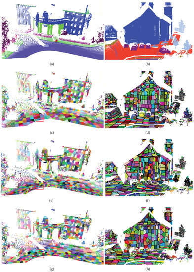
Figure 14.
Visual comparisons using the point clouds from the Oakland (left) and Semantic3D (right) datasets. (a,b) Ground truth; (c,d) the VCCS results; (e,f) the BPSS results; and (g,h): our merge-swap results. Unlabelled points are not shown in the ground truth.
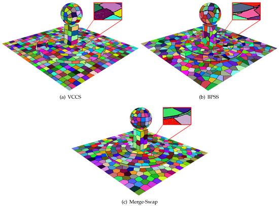
Figure 15.
Compactness comparison. Our merge-swap result produced the best compactness in flat regions.
5.4. Running Time
The timings versus data point numbers of the compared algorithms are plotted in Figure 16. The input point clouds had different numbers of points sampled from the same scene, and the output number of supervoxels was fixed to 1,000. The times for data I/O and building the k-d tree were not included for the three methods. The time for building the octree in our method was included. We ran each program 10 times and computed the average running time. Figure 16 shows the VCCS method is the most efficient approach as the original problem is reduced to that of generating supervoxels for a smaller number of regular voxels, resulting in corresponding quality sacrifices. Whereas the BPSS method acts directly on the original points, the proposed method adopts an adaptive octree to cluster the original points into fine voxels and starts the merging process from these fine voxels. When the number of points is large, it produces an obvious acceleration effect. Figure 16 shows that our method is more efficient than the BPSS method when the data size grows to over 10 million, with improved supervoxel qualities. In addition, the complexity of a scene has an effect on the efficiency of the proposed method, leading to an octree with a different number of nodes.
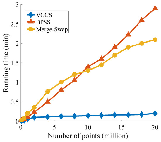
Figure 16.
Comparison of running time for the VCCS method, the BPSS method, and our merge-swap method.
6. Summary and Conclusions
In this paper, we presented our proposed merge-swap framework—a simple supervoxel generation algorithm for point clouds. The framework consists of two stages: merging and swapping. In the merging stage, the number of supervoxels is reduced by iteratively merging two supervoxels with the minimal cost into one. To find the supervoxel pair with the minimal cost in each iteration, we propose to maintain a dynamic min-heap, which is large when processing large-scale point clouds. Thus, we also presented two acceleration techniques to reduce the size of the min-heap and the speedup ratio is considerable. In the swapping stage, each boundary point is tested to see if it can be swapped with its neighboring supervoxel. This operation is crucial for further reducing the total energy value of the supervoxels.
The proposed merge-swap method can be used for solving any supervoxel generation problem that is formulated in energy minimization. In particular, an energy function is tailored to explicitly encourage compact supervoxels with a size control adaptive to local geometric information of point clouds. The control of other properties of supervoxels in the energy function can also be incorporated. Experimental results, including performance comparisons on three public datasets and several visual comparisons on point clouds, demonstrated that our merge-swap method produces supervoxels at a lower computational cost while producing a better segmentation quality than the state-of-the-art BPSS method.
Despite the proposed merge-swap method preserveing sharp features significantly better than two state-of-the-art supervoxel methods, it suffers from one major limitation: our merge-swap method is less efficient than the VCCS method, which may limit its use in practical applications. Hence, a future work direction is to develop parallel algorithms of the merge-swap method to further improve the efficiency. The proposed method requires extra memory to save min-heaps, requiring about 6 GB memory to process 10 million points, and it is quite common for a terrestrial LiDAR scan to have billions of points, As the merging and the swapping operations could be applied locally to a point cloud, a possible solution is to divide a large-scale point cloud into smaller parts and perform our framework on each part individually, and then merge the results. We leave this for future work. We would also like to explore the applications of our method to other point cloud processing problems, i.e., line/plane structures extraction, segmentation, and classification.
Author Contributions
Conceptualization, Z.C.; Methodology, Y.X. and Z.C.; Software, Y.X., Z.L., and Y.L.; Supervision, Y.J.Z., and C.W.; Validation, Y.X., Z.C., and J.C.; Visualization, Y.X. and Z.L.; Writing–original draft, Y.X.; Writing–review and editing, Z.C., J.C., Y.J.Z., and C.W. All authors have read and agree to the published version of the manuscript.
Funding
Zhonggui Chen and Juan Cao were funded by the National Natural Science Foundation of China (Nos. 61872308, 61972327), the Natural Science Foundation of Fujian Province of China (Nos. 2018J01104, 2019J01026), and the Fundamental Research Funds for the Central Universities (Nos. 20720190011, 20720190063). Yongjie Jessica Zhang was funded in part by the PECASE Award N00014-16-1-2254. Yangbin Lin was funded by the National Natural Science Foundation of China (No. 61701191). Cheng Wang was funded in part by the National Natural Science Foundation of China (No. U1605254).
Acknowledgments
Part of this work was done when Yanyang Xiao was visiting the Department of Mechanical Engineering, Carnegie Mellon University.
Conflicts of Interest
The authors declare no conflict of interest.
References
- Luo, H.; Wang, C.; Wen, C.; Cai, Z.; Chen, Z.; Wang, H.; Yu, Y.; Li, J. Patch-based semantic labeling of road scene using colorized mobile LiDAR point clouds. IEEE Trans. Intell. Transp. Syst. 2016, 17, 1286–1297. [Google Scholar] [CrossRef]
- Sun, Z.; Xu, Y.; Hoegner, L.; Stilla, U. Classification of MLS point clouds in urban scenes using detrended geometric features from supervoxel-based local contexts. ISPRS Ann. Photogramm. Remote. Sens. Spat. Inf. Sci. 2018, IV-2, 271–278. [Google Scholar] [CrossRef]
- Yun, J.S.; Sim, J.Y. Supervoxel-based saliency detection for large-scale colored 3D point clouds. In Proceedings of the IEEE International Conference on Image Processing, Phoenix, AZ, USA, 25–28 September 2016; pp. 4062–4066. [Google Scholar]
- Wang, H.; Wang, C.; Luo, H.; Li, P.; Chen, Y.; Li, J. 3-D point cloud object detection based on supervoxel neighborhood with Hough forest framework. IEEE J. Sel. Top. Appl. Earth Obs. Remote. Sens. 2015, 8, 1570–1581. [Google Scholar] [CrossRef]
- Ban, Z.; Chen, Z.; Liu, J. Supervoxel segmentation with voxel-related gaussian mixture model. Sensors 2018, 18, 128. [Google Scholar]
- Tian, Z.; Liu, L.; Zhang, Z.; Xue, J.; Fei, B. A supervoxel-based segmentation method for prostate MR images. Med Phys. 2017, 44, 558–569. [Google Scholar] [CrossRef]
- Achanta, R.; Shaji, A.; Smith, K.; Lucchi, A.; Fua, P.; Süsstrunk, S. SLIC superpixels compared to state-of-the-art superpixel methods. IEEE Trans. Pattern Anal. Mach. Intell. 2012, 34, 2274–2282. [Google Scholar] [CrossRef]
- Papon, J.; Abramov, A.; Schoeler, M.; Wörgötter, F. Voxel cloud connectivity segmentation - supervoxels for point clouds. In Proceedings of the IEEE Conference on Computer Vision and Pattern Recognition, Portland, OR, USA, 23–28 June 2013; pp. 2027–2034. [Google Scholar]
- Lin, Y.; Wang, C.; Zhai, D.; Li, W.; Li, J. Toward better boundary preserved supervoxel segmentation for 3D point clouds. ISPRS J. Photogramm. Remote. Sens. 2018, 143, 39–47. [Google Scholar] [CrossRef]
- Hu, K.; Zhang, Y.J. Image segmentation and adaptive superpixel generation based on harmonic edge-weighted centroidal Voronoi tessellation. Comput. Methods Biomech. Biomed. Eng. Imaging Vis. 2016, 4, 46–60. [Google Scholar] [CrossRef]
- Dong, X.; Chen, Z.; Yao, J.; Guo, X. Superpixel generation by agglomerative clustering with quadratic error minimization. Comput. Graph. Forum 2019, 38, 405–416. [Google Scholar] [CrossRef]
- Pan, X.; Zhou, Y.; Chen, Z.; Zhang, C. Texture relative superpixel generation with adaptive parameters. IEEE Trans. Multimed. 2019, 21, 1997–2011. [Google Scholar] [CrossRef]
- Stutz, D.; Hermans, A.; Leibe, B. Superpixels: An evaluation of the state-of-the-art. Comput. Vis. Image Underst. 2018, 166, 1–27. [Google Scholar] [CrossRef]
- Weikersdorfer, D.; Gossow, D.; Beetz, M. Depth-adaptive superpixels. In Proceedings of the 21st International Conference on Pattern Recognition, Tsukuba, Japan, 11–15 November 2012; pp. 2087–2090. [Google Scholar]
- Liu, Y.J.; Yu, C.C.; Yu, M.J.; He, Y. Manifold SLIC: A fast method to compute content-sensitive superpixels. In Proceedings of the IEEE Conference on Computer Vision and Pattern Recognition, Las Vegas, NV, USA, 27–30 June 2016; pp. 651–659. [Google Scholar]
- Pan, X.; Zhou, Y.; Li, F.; Zhang, C. Superpixels of RGB-D images for indoor scenes based on weighted geodesic driven metric. IEEE Trans. Vis. Comput. Graph. 2017, 23, 2342–2356. [Google Scholar] [CrossRef] [PubMed]
- Gao, G.; Lauri, M.; Zhang, J.; Frintrop, S. Saliency-guided adaptive seeding for supervoxel segmentation. In Proceedings of the IEEE/RSJ International Conference on Intelligent Robots and Systems, Vancouver, BC, Canada, 24–28 September 2017; pp. 4938–4943. [Google Scholar]
- Liu, Y.; Yu, M.; Li, B.; He, Y. Intrinsic manifold SLIC: A simple and efficient method for computing content-sensitive superpixels. IEEE Trans. Pattern Anal. Mach. Intell. 2018, 40, 653–666. [Google Scholar] [CrossRef] [PubMed]
- Yang, J.; Gan, Z.; Gui, X.; Li, K.; Hou, C. 3-D geometry enhanced superpixels for RGB-D data. In Proceedings of the Advances in Multimedia Information Processing—PCM, 14th Pacific-Rim Conference on Multimedia, Nanjing, China, 13–16 December 2013; pp. 35–46. [Google Scholar]
- Cai, Y.; Guo, X.; Zhong, Z.; Mao, W. Dynamic meshing for deformable image registration. Comput.-Aided Des. 2015, 58, 141–150. [Google Scholar] [CrossRef]
- Cai, Y.; Guo, X. Anisotropic superpixel generation based on Mahalanobis distance. Comput. Graph. Forum. 2016, 35, 199–207. [Google Scholar] [CrossRef]
- Song, S.; Lee, H.; Jo, S. Boundary-enhanced supervoxel segmentation for sparse outdoor LiDAR data. Electron. Lett. 2014, 50, 1917–1919. [Google Scholar] [CrossRef]
- Kim, J.S.; Park, J.H. Weighted-graph-based supervoxel segmentation of 3D point clouds in complex urban environment. Electron. Lett. 2015, 51, 1789–1791. [Google Scholar] [CrossRef]
- Che, E.; Jung, J.; Olsen, M.J. Object recognition, segmentation, and classification of mobile laser scanning point clouds: A state of the art review. Sensors 2019, 19, 810. [Google Scholar] [CrossRef]
- Hoppe, H.; DeRose, T.; Duchamp, T.; McDonald, J.; Stuetzle, W. Surface reconstruction from unorganized points. In Proceedings of the 19th Annual Conference on Computer Graphics and Interactive Techniques, Seattle, WA, USA, 27–31 July 1992; pp. 71–78. [Google Scholar]
- Du, Q.; Faber, V.; Gunzburger, M. Centroidal Voronoi tessellations: Applications and algorithms. SIAM Rev. 1999, 41, 637–676. [Google Scholar] [CrossRef]
- Whang, K.Y.; Song, J.W.; Chang, J.W.; Kim, J.Y.; Cho, W.S.; Park, C.M.; Song, I.Y. Octree-R: An adaptive octree for efficient ray tracing. IEEE Trans. Vis. Comput. Graph. 1995, 1, 343–349. [Google Scholar] [CrossRef]
- Vo, A.V.; Truong-Hong, L.; Laefer, D.F.; Bertolotto, M. Octree-based region growing for point cloud segmentation. ISPRS J. Photogramm. Remote. Sens. 2015, 104, 88–100. [Google Scholar] [CrossRef]
- Zhang, Y.J. Geometric Modeling and Mesh Generation from Scanned Images, 1st ed.; Chapman and Hall/CRC: Boca Raton, FL, USA, 2016; pp. 107–134. [Google Scholar]
- Zhang, Y.; Bajaj, C.; Sohn, B.S. 3D finite element meshing from imaging data. Comput. Methods Appl. Mech. Eng. 2005, 194, 5083–5106. [Google Scholar] [CrossRef] [PubMed]
- Zhang, Y.; Bajaj, C. Adaptive and quality quadrilateral/hexahedral meshing from volumetric data. Comput. Methods Appl. Mech. Eng. 2006, 195, 942–960. [Google Scholar] [CrossRef] [PubMed]
- Zhang, Y.; Hughes, T.J.; Bajaj, C.L. An automatic 3D mesh generation method for domains with multiple materials. Comput. Methods Appl. Mech. Eng. 2010, 199, 405–415. [Google Scholar] [CrossRef]
- Chernyshenko, A.Y.; Olshanskii, M.A. An adaptive octree finite element method for PDEs posed on surfaces. Comput. Methods Appl. Mech. Eng. 2015, 291, 146–172. [Google Scholar] [CrossRef]
- Marco, O.; Sevilla, R.; Zhang, Y.; Ródenas, J.J.; Tur, M. Exact 3D boundary representation in finite element analysis based on Cartesian grids independent of the geometry. Int. J. Numer. Methods Eng. 2015, 103, 445–468. [Google Scholar] [CrossRef]
- Silberman, N.; Hoiem, D.; Kohli, P.; Fergus, R. Indoor segmentation and support inference from RGBD images. In Proceedings of the European Conference on Computer Vision, Florence, Italy, 7–13 October 2012; pp. 746–760. [Google Scholar]
- Munoz, D.; Bagnell, J.A.D.; Vandapel, N.; Hebert, M. Contextual classification with functional max-margin Markov networks. In Proceedings of the IEEE Computer Society Conference on Computer Vision and Pattern Recognition, Miami, FL, USA, 20–25 June 2009. [Google Scholar]
- Hackel, T.; Savinov, N.; Ladicky, L.; Wegner, J.D.; Schindler, K.; Pollefeys, M. SEMANTIC3D.NET: A new large-scale point cloud classification benchmark. In Proceedings of the ISPRS Annals of the Photogrammetry, Remote Sensing and Spatial Information Sciences, ISPRS Hannover Workshop, Hannover, Germany, 6–7 June 2017; pp. 91–98. [Google Scholar]
- Martin, D.R.; Fowlkes, C.C.; Malik, J. Learning to detect natural image boundaries using local brightness, color, and texture cues. IEEE Trans. Pattern Anal. Mach. Intell. 2004, 26, 530–549. [Google Scholar] [CrossRef]
- Levinshtein, A.; Stere, A.; Kutulakos, K.N.; Fleet, D.J.; Dickinson, S.J.; Siddiqi, K. TurboPixels: Fast superpixels using geometric flows. IEEE Trans. Pattern Anal. Mach. Intell. 2009, 31, 2290–2297. [Google Scholar] [CrossRef]
- Martin, D.; Fowlkes, C.; Tal, D.; Malik, J. A database of human segmented natural images and its application to evaluating segmentation algorithms and measuring ecological statistics. In Proceedings of the Eighth IEEE International Conference on Computer Vision, Vancouver, BC, Canada, 7–14 July 2001; pp. 416–423. [Google Scholar]
- Schick, A.; Fischer, M.; Stiefelhagen, R. An evaluation of the compactness of superpixels. Pattern Recognit. Lett. 2014, 43, 71–80. [Google Scholar] [CrossRef]
© 2020 by the authors. Licensee MDPI, Basel, Switzerland. This article is an open access article distributed under the terms and conditions of the Creative Commons Attribution (CC BY) license (http://creativecommons.org/licenses/by/4.0/).