A Two-Stream Symmetric Network with Bidirectional Ensemble for Aerial Image Matching

Abstract

In this paper, we propose a novel method to precisely match two aerial images that were obtained in different environments via a two-stream deep network. By internally augmenting the target image, the network considers the two-stream with the three input images and reflects the additional augmented pair in the training. As a result, the training process of the deep network is regularized and the network becomes robust for the variance of aerial images. Furthermore, we introduce an ensemble method that is based on the bidirectional network, which is motivated by the isomorphic nature of the geometric transformation. We obtain two global transformation parameters without any additional network or parameters, which alleviate asymmetric matching results and enable significant improvement in performance by fusing two outcomes. For the experiment, we adopt aerial images from Google Earth and the International Society for Photogrammetry and Remote Sensing (ISPRS). To quantitatively assess our result, we apply the probability of correct keypoints (PCK) metric, which measures the degree of matching. The qualitative and quantitative results show the sizable gap of performance compared to the conventional methods for matching the aerial images. All code and our trained model, as well as the dataset are available online.

1. Introduction

1.1. Motivation

Aerial image matching is a geometric process of aligning a source image with a target image. Both images display the same scene but are obtained in different environments, such as time, viewpoints and sensors. It also a prerequisite of a variety of aerial image tasks such as change detection, image fusion, and image stitching. Since it can have a significant impact on the performance of the following tasks, it is an extremely important task. As shown in Figure 1, various environments have considerable visual differences of land-coverage, weather, and objects. The variance in the aerial images causes degradation of the matching precision. In conventional computer vision approaches, correspondences between two images are computed by the hand-crafted algorithm (such as SIFT [1], SURF [2], HOG [3], and ASIFT [4]), followed by estimating the global geometric transformation using RANSAC [5] or Hough transform [6,7]. However, these approaches are not very successful for aerial images due to their high-resolution, computational costs, large-scale transformation, and variation in the environments.

Another problem with aerial image matching is the asymmetric result. As aforementioned, there are tons of aerial image matching methods [1,2,3,4,5,6,7]. Notwithstanding, these methods [1,2,3,4,5,6,7] have overlooked the consistency of matching flow. i.e., most methods consider only one direction of the matching flows (from source to target). It causes asymmetric matching results and degradation of the overall performance. In Figure 2, it illustrates a failure case when the source image and the target image are swapped.

Many computer vision tasks have been applied and developed in real life [8,9,10,11,12,13,14,15,16,17,18,19,20,21,22,23,24]. Because deep neural networks (DNNs) have shown impressive performance in real-world computer vision tasks [25,26,27,28], several approaches apply DNNs to overcome the limitation of traditional computer vision methods for matching the images. The Siamese network [29,30,31,32] has been extensively applied to extract important features and to match image-patch pairs [33,34,35]. Furthermore, several works [36,37,38] apply an end-to-end manner in the geometric matching area. While numerous matching tasks have been actively explored with deep learning, few approaches utilize DNNs in aerial image matching areas.

In this work, we utilize a deep end-to-end trainable matching network and design a two-stream architecture to address the variance in the aerial images obtained in diverse environments. By internally augmenting the target image and considering the three inputs, we regularize the training process, which produces a more generalized deep network. Furthermore, our method is designed as a bidirectional network with an efficient ensemble manner. Our ensemble method is inspired by the isomorphic nature of the geometric transformation. We apply this method in our inference procedure without any additional networks or parameters. The ensemble approach also assists in alleviating the variance between estimated transformation parameters from both directions. Figure 3 illustrates an overview of our proposed method.

1.2. Contibutions

To sum up, our contributions are three-fold:

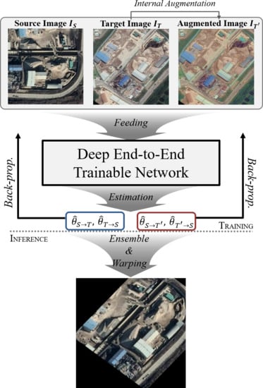
• For aerial image matching, we propose a deep end-to-end trainable network with a two-stream architecture. The three inputs are constructed by internal augmentation of the target image, which regularizes the training process and overcomes the shortcomings of the aerial images due to various capturing environments.
• We introduce a bidirectional training architecture and an ensemble method, inspired by the isomorphism of the geometric transformation. It alleviates the asymmetric result of image matching. The proposed ensemble method assists the deep network to become robust for the variance between estimated transformation parameters from both directions and shows improved performance in evaluation without any additional network or parameters.
• Our method shows more stable and precise matching results from the qualitative and quantitative assessment. In the aerial image matching domain, we first apply probability of correct keypoints (PCK) metrics [44] to objectively assess quantitative performance with a large volume of aerial images. Our dataset, model and source code are available at https://github.com/jaehyunnn/DeepAerialMatching.

1.3. Related Works

In general, the image matching problem has been addressed in two types of methods: area-based methods and feature-based methods [39,40]. The former methods investigate the correspondence between two images using pixel intensities. However, these methods are vulnerable to noise and variation in illumination. The latter methods extract the salient features from the images to solve these drawbacks.

Most classical pipelines for matching two images consist of three stages, (1) feature extraction, (2) feature matching, and (3) regression of transformation parameters. As conventional matching methods, hand-crafted algorithms [1,2,3,4] are extensively used to extract local features. However, these methods often fail for large changes in situations, which is attributed to the lack of generality for various tasks and image domains.

Convolutional neural networks (CNNs) have shown tremendous strength for extracting high-level features to solve various computer vision tasks, such as semantic segmentation [27,41], object detection [26,42], classification [25,43], human action recognition [44,45], and matching. In the field of matching, E. Simo-Serra et al. [33] learned local features based on image-patch with a Siamese network and use the L2-distance for the loss function. X. Han et al. [35] proposed a feature network and metric network to match two image patches. S. Zagoruyko et al. [34] expanded the Siamese network in two-streams: surround stream and central stream. K.-M Yi et al. [46] proposed a framework that includes detection, orientation, estimation, and description by mimicking SIFT [1]. H. Altwaijry et al. [31] performed ultra-wide baseline aerial image matching with a deep network and spatial transformer module [47]. H. Altwaijry et al. [48] also proposed a deep triplet architecture that learns to detect and match keypoints with 3-D keypoints ground-truth extracted by VisualSFM [49,50]. I. Rocco et al. [36] first proposed a deep network architecture for geometric matching, and demonstrated the advantage of a deep end-to-end network by achieving 57% PCK score in the semantic alignment. This method constructs a dense-correspondence map using two image features and directly regress the transformation parameters. These researchers further proposed a weakly-supervision approach that does not require any additional ground-truth for training [37]. P. Seo et al. [38] applied an attention mechanism with an offset-aware correlation (OAC) kernel based on [36] and achieved a 68% PCK score.

Although these works show meaningful results, their accuracy or computational costs for aerial image matching require improvement. Therefore, we compose a matching network that is suitable for aerial images by pruning the factors that degrade performance.

2. Materials and Methods

We propose a deep end-to-end trainable network with a two-stream architecture and bidirectional ensemble method for aerial image matching. Our proposed network focuses on addressing the variance in the aerial images and asymmetric matching results. The steps for predicting transformation are listed as follows: (1) internal augmentation, (2) feature extraction with the backbone network, (3) correspondence matching, (4) regression of transformation parameters, and (5) application of ensemble to the multiple outcomes. In Figure 4, we present the overall architecture of the proposed network.

2.1. Internal Augmentation for Regularization

The network considers two aerial images (source image $I_S$ and target image $I_T$) with different temporal and geometric properties as the input. By using this original pair $(I_S,I_T)$ in the training process, the deep network is trained by considering the relation of only two images obtained in different environments. However, this approach is insufficient for addressing the variance in the aerial images. Collecting various pair sets to solve these problems is expensive. To address this issue, we augment the target image by internally jittering image color during the training procedure. The network can be trained with various image pairs since the color of the target image is randomly jittered in every training iteration as shown in Figure 5. This step has a regularization effect of the training process, which produces a more generally trained network. The constructed three inputs are passed through a deep network. Subsequently, the network directly and simultaneously estimates global geometrical transformation parameters for the original pair and augmented pair. Note that the internal augmentation is only performed in the training procedure. In inference procedure, we utilize a single-stream architecture without the internal augmentation process for computational efficiency.

2.2. Feature Extraction with Backbone Network

Given the input images $(I_S,I_T,I_{T^{\prime }})\in {\mathbb{R}}^{h\times w\times d}$, we extract their feature maps $(f_S,f_T,f_{T^{\prime }})\in {\mathbb{R}}^{h^{\prime }\times w^{\prime }\times d^{\prime }}$ by passing a fully-convolutional backbone network $\mathcal{F}$, which is expressed as follows:

$$\mathcal{F}:{\mathbb{R}}^{h\times w\times d}\to {\mathbb{R}}^{h^{\prime }\times w^{\prime }\times d^{\prime }},$$

(1)

where $(h,w,d)$ denote the heights, widths, and dimensions of the input images and $(h^{\prime },w^{\prime },d^{\prime })$ are those of the extracted features, respectively.

We investigate various models of the backbone networks, as shown in Section 3. SE-ResNeXt101 [43] add the Squeeze-and-Excitation (SE) block as the channel-attention module to ResNeXt101 [51], which has shown its superiority in [52]. Figure 6 shows the SE-block. Therefore, we leverage SE-ResNeXt101 as the backbone network and empirically show that it has an important role in improving performance compared with other backbone networks. We utilize the image features extracted from layer-3 in the backbone network and apply L2-normalization to extracted features.

2.3. Correspondence Matching

As a method for computing a dense-correspondence map between two feature maps [36], the matching function $\mathcal{C}$ is expressed as follows:

$$\begin{array}{cc}\hfill c_{S\to T}(i,j,k)& =\mathcal{C}(f_S(i_k,j_k),f_T(i,j))\hfill \\ \hfill & =f_T{(i,j)}_S^f(i_k,j_k),\hfill \end{array}$$

(2)

where $c_{S\to T}$ is the dense-correspondence map that matches the source feature map $f_S$ to the target feature map $f_T$. $(i,j)$ and $(i_k,j_k)$ indicate the coordinate of each feature point in the feature maps. Each element in $c_{S\to T}$ refers to the similarity score between two points.

We construct the dense-correspondence map of the original pair and augmented pair. To consider only positive values for ease of training, the negative scores in the dense-correspondence map are removed by ReLU non-linearity, followed by L2-normalization.

2.4. Regression of Transformation Parameters

The regression step is for predicting the transformation parameters. When the dense-correspondence maps are passed through the regression network $\mathcal{R}$, the network $\mathcal{R}$ directly estimates the geometric transformation parameters as follows:

$$\mathcal{R}:{\mathbb{R}}^{h^{\prime }\times w^{\prime }\times (h^{\prime }\times w^{\prime })}\to {\mathbb{R}}^{DoF},$$

(3)

where $(h^{\prime },w^{\prime })$ indicate the heights and widths of the feature maps, and $DoF$ means the degrees of freedom of the transformation model.

We adopt the affine transformation which has 6-$DoF$ and the ability to preserve straight lines. In the semantic alignment domain [36,37,38], thin-plate spline (TPS) transformation [53] which has 18-$DoF$ is used to improve the performance. However, it is not suitable in the aerial image matching domain, because it produces large distortions of the straight lines (such as roads and boundaries of the buildings). Therefore, we infer the six parameters that handle the affine transformation.

2.5. Ensemble Based on Bidirectional Network

The affine transformation is invertible due to its isomorphic nature. We take advantage of this characteristic to design a bidirectional network and apply an ensemble approach. Applying the ensemble method enables alleviating the variance in the aerial images and improvement in the matching performance without any additional networks or models.

2.5.1. Bidirectional Network

Inspired by its isomorphic nature, we expand the base architecture by adding a branch that symmetrically estimates the transformation in the opposite direction symmetrically. The network yields the transformation parameters in both directions of each pair, i.e., $({\widehat{\theta }}_{S\to T},{\widehat{\theta }}_{T\to S})$ and $({\widehat{\theta }}_{S\to T^{\prime }},{\widehat{\theta }}_{T^{\prime }\to S})$. To infer the parameters of another branch, we compute the dense-correspondence map in the opposite direction by using the same method as in Section 2.3. All dense-correspondence maps are passed through the identical regression network $\mathcal{R}$. Since we utilize a regression network for all cases, no additional parameters are needed in this procedure. The proposed bidirectional network only adds a small amount of computational overhead compared with the base architecture.

2.5.2. Ensemble

In general, the ensemble technique requires several additional different architectures and consumes additional time costs to train models differently. We introduce an efficient ensemble method without any additional architectures or models by utilizing the isomorphism of the affine transformation. Figure 7 illustrates the overview of the ensemble procedure. ${({\widehat{\theta }}_{T\to S})}^{-1}$, which is the inverse of ${\widehat{\theta }}_{T\to S}$, can be expressed as another transformation parameters in the direction from $I_S$ to $I_T$. To compute ${({\widehat{\theta }}_{T\to S})}^{-1}$, we convert ${\widehat{\theta }}_{T\to S}$ into the homogeneous form:

$$[a_1,a_2,t_x,a_3,a_4,t_y]⟹\left[\begin{array}{ccc}{a}_1& a_2& t_x\\ a_3& a_4& t_y\\ 0& 0& 1\end{array}\right].$$

(4)

In the affine transformation parameters $[a_1,a_2,t_x,a_3,a_4,t_y]$, $a_1\sim a_4$ represent the scale, rotated angle and tilted angle, and $(t_x,t_y)$ denotes the $(x$-axis, y-axis) translation. We compute ${({\widehat{\theta }}_{T\to S})}^{-1}$ by converting the homogeneous form, as shown in Equation (4). This inverse matrix denotes another affine transformation from $I_S$ to $I_T$. As a result, we fuse the two sets of affine transformation parameters as follows:

$${\widehat{\theta }}_{en}=\mu ({\widehat{\theta }}_{S\to T},{({\widehat{\theta }}_{T\to S})}^{-1}),$$

(5)

where $\mu (\ast )$ denotes the mean function for fusing two parameters. In the various experiments, we apply three types of mean: arithmetic mean, harmonic mean and geometric mean. Empirically, arithmetic mean shows the best performance. In the inference process, ${\widehat{\theta }}_{en}$ warps the source image into the target image. Note that we fuse only parameters that correspond to the original pair since we use the original two-stream network in the inference procedure and do not utilize the ensembled parameters in the training procedure to maximize the ensemble effects.

2.6. Loss Function

In the training procedure, we adopt the transformed grid loss [36] as the baseline loss function. Given the predicted transformation $\widehat{\theta }$ and the ground-truth ${\theta }^{gt}$, the baseline loss function $l(\widehat{\theta },{\theta }^{gt})$ is obtained by the following:

$$l(\widehat{\theta },{\theta }^{gt})=\frac{1}{N}\sum _{i,j=1}^{N}d{({\mathcal{T}}_{\widehat{\theta }}(x_i,y_j),{\mathcal{T}}_{{\theta }^{gt}}(x_i,y_j))}^2,$$

(6)

where N is the number of grid points, ${\mathcal{T}}_{\widehat{\theta }}(\ast )$ and ${\mathcal{T}}_{{\theta }^{gt}}(\ast )$ are the transforming operations parameterized by $\widehat{\theta }$ and ${\theta }^{gt}$, respectively. To achieve bidirectional learning, we add a term for training the additional branch to the baseline loss function. Formally, we define the proposed bidirectional loss of the original pair, ${\mathcal{L}}_{org}$, as follows:

$$\begin{array}{cc}\hfill {\mathcal{L}}_{org}=& l({\widehat{\theta }}_{S\to T},{\theta }_{S\to T}^{gt})+l({\widehat{\theta }}_{T\to S},{({\theta }_{S\to T}^{gt})}^{-1}).\hfill \end{array}$$

(7)

Note that additional ground-truth information for the opposite direction is not required due to the isomorphism of the affine transformation. For regularization of training, we add two terms utilizing the augmented pair:

$$\begin{array}{cc}\hfill {\mathcal{L}}_{aug}=& l({\widehat{\theta }}_{S\to T^{\prime }},{\theta }_{S\to T}^{gt})+l({\widehat{\theta }}_{T^{\prime }\to S},{({\theta }_{S\to T}^{gt})}^{-1}),\hfill \end{array}$$

(8)

$$\begin{array}{cc}\hfill {\mathcal{L}}_{id}=& l({\widehat{\theta }}_{S\to T},{\theta }_{S\to T^{\prime }})+l({\widehat{\theta }}_{T\to S},{\theta }_{T^{\prime }\to S}).\hfill \end{array}$$

(9)

The augmented pair also share the ground-truth since the geometric relation between two images is equivalent to the original pair. The identity term in Equation (9) induces training to ensure that the prediction values from the original pair and the augmented pair are equal. Our proposed final loss function is defined by the following:

$$\begin{array}{cc}\hfill \mathcal{L}=& \alpha ·{\mathcal{L}}_{org}+\beta ·{\mathcal{L}}_{aug}+\gamma ·{\mathcal{L}}_{id},\hfill \end{array}$$

(10)

where $(\alpha ,\beta ,\gamma )$ are the balance parameters of each loss term. In our experiment, we set these parameters to (0.5, 0.3, 0.2), respectively.

3. Results

In this section, we present the implementation details, experiment settings, and results. For the quantitative evaluation, we compare the proposed method with other methods for aerial image matching. We further experiment with various backbone networks to obtain more suitable features for our work. We show the contributions of each proposed component in the ablation study section and the qualitative results of the proposed network compared with other networks.

3.1. Implementation Details

We implemented the proposed network using PyTorch [54] and trained our model with the ADAM optimizer [55], using a learning rate $5\times {10}^{-4}$ and a batch size of 10. We further performed data augmentation by generating the random affine transformation as the ground-truth. All input images were resized to $240\times 240$.

3.2. Experimental Settings

3.2.1. Training

We generated the training input pairs by applying random affine transformations to the multi-temporal aerial image pairs captured in Google Earth. Since no datasets were annotated with completely correct transformation parameters between two images, we built the training dataset, 9000 multi-temporal aerial image pairs, and corresponding ground-truths. Basically, multi-tempral image pairs consisted of the image pairs which were taken at different times (2019, 2017, and 2015) and by different sensors (Landsat-7, Landsat-8, WorldView, and QuickBird). The process of annotating ground-truth is as follows: (1) we employed the multi-temporal image pairs $(I,I^{\prime })$ with the same region and viewpoint. (2) The first images in the multi-temporal aerial image pairs were center-cropped. (3) The second images are transformed by the randomly generated affine transformation ${\theta }_{S\to T}^{gt}$ which was used as a ground-truth and subsequently center-cropped. (4) The center-crop process was performed to exclude the black area that serves as noise after transformation. Figure 8 illustrates the process of generating training pairs and ground-truths. In Algorithm 1, the training procedure is detailed. It has $O(N)$ complexity with respect to the number of training pairs N. We train our model for 2-days on a single NVIDIA Titan V GPU.

Algorithm 1: Training procedure.

Input: Training aerial image dataset D        Randomly initialized model ${\mathcal{M}}_w$    Output: Trained model ${\mathcal{M}}_w$    for epochs do        end

3.2.2. Evaluation

To demonstrate the superiority of our method quantitatively, we evaluated our model using the PCK [56], which was extensively applied in the other matching tasks [36,37,38,57,58,59,60]. PCK metric is defined as follows:

$$PCK=\frac{{\sum }_{i=1}^n{\sum }_{p_i}1[d({\mathcal{T}}_{\widehat{\theta }}(p_i),{\mathcal{T}}_{{\theta }^{gt}}(p_i))<\tau ·max(h,w)]}{{\sum }_{i=1}^n\left|p_i\right|},$$

(11)

where $p_i$ is the ith point, which consists of $(x_i,y_i)$, and $\tau ·\max (h,w)$ refers to the tolerance term in the image size of $h\times w$. Intuitively, the denominator and the numerator denote the number of correct keypoints and overall annotated keypoints, respectively. The PCK metric shows how well matching is successful globally according to given $\tau$ with a lot of test images. In this evaluation, we assess in the cases of $\tau =0.1,0.3,$ and $0.5$. The greater value of $\tau$ allows measuring degrees of matching more globally. To adopt the PCK metric, we annotated the keypoints and ground-truth transformation to 500 multi-temporal aerial image pairs. The multi-temporal pairs are captured in Google Earth and composed of major administrative districts in South Korea, like the training image pairs. The annotation process is as the following process: (1) we extracted the keypoints of multi-temporal aerial image pairs using SIFT [1], and (2) picked up the overlapping keypoints between each image pair. We annotate 20 keypoints per image pair, which generate a total of 10k keypoints for a quantitative assessment. This approach provides a fair demonstration of quantitative performance. In the evaluation and the inference procedure, we used a two-stream network, except for the augmented branch shown in Algorithms 2.

Algorithm 2: Inference procedure.

Input: Source and target images $(I_S,I_T)$       Trained model ${\mathcal{M}}_w$    Output: Transformed image $I_S^{\prime }$    # Feed-forward    ${\widehat{\theta }}_{S\to T},{\widehat{\theta }}_{T\to S}={\mathcal{M}}_w(I_S,I_T)$;    # Ensemble    ${\widehat{\theta }}_{en}=\mu ({\widehat{\theta }}_{S\to T},{({\widehat{\theta }}_{T\to S})}^{-1})$;    # Transform source image to target image    $I_S^{\prime }={\mathcal{T}}_{{\widehat{\theta }}_{en}}(I_S)$

3.3. Results

3.3.1. Quantitative results

Aerial Image Dataset

Table 1. Comparisons of probability of correct keypoints (PCK) in the aerial images. CNNGeo is evaluated in two versions: the pre-trained model provided in [36] and the fine-tuned model by the aerial images. Both models use ResNet101 as the backbone network.

Methods	PCK (%)
	$\mathbf{\tau }=0.05$	$\mathbf{\tau }=0.03$	$\mathbf{\tau }=0.01$
SURF [2]	26.7	23.1	15.3
SIFT [1]	51.2	45.9	33.7
ASIFT [4]	64.8	57.9	37.9
OA-Match [61]	64.9	57.8	38.2
CNNGeo [36] (pretrained)	17.8	10.7	2.5
CNNGeo (fine-tuned)	90.6	76.2	27.6
Ours; ResNet101 [62]	93.8	82.5	35.1
Ours; ResNeXt101 [51]	94.6	85.9	43.2
Ours; Densenet169 [63]	95.6	88.4	44.0
Ours; SE-ResNeXt101 [43]	97.1	91.1	48.0

shows quantitative comparisons to the conventional computer vision methods (SURF [2], SIFT [1], ASIFT [4] + RANSAC [5] and OA-Match [61]) and CNNGeo [36] on aerial image data with large transformation. Conventional computer vision methods [1,2,4,5,61] showed quite a number of critical failures globally. As shown in Table 1, the conventional methods show low PCK performance in the case of $\tau =0.05$. However, in the case of $\tau =0.01$, these methods showed lower degradation of performance compared with other deep learning based methods. This result implies that conventional methods enable finer matching if the matching procedure does not failed entirely. Although CNNGeo fine-tuned by aerial images shows somewhat tolerable performance, our method considerably outperforms this method in all cases of $\tau$. Furthermore, we performed an investigation of the various backbone networks to demonstrate the importance of feature extraction. Since the backbone network substantially affects the total performance, we experimentally adopted the best backbone network.

Ablation Study

The proposed method combines two distinct techniques: (1) internal augmentation and (2) bidirectional ensemble. We analyze the contributions and effects of each proposed component and compare our models with CNNGeo [36]. ’+ Int. Aug.’ and ’+ Bi-En.’, which signify the internal augmentation and bidirectional ensemble addition, respectively. As shown in

Table 2. Results of models with different additional components. We analyzed the contributions of each component with ResNet-101 backbone.

Methods	PCK (%)
	$\mathbf{\tau }=0.05$	$\mathbf{\tau }=0.03$	$\mathbf{\tau }=0.01$
CNNGeo [36]	90.6	76.2	27.6
CNNGeo + Int. Aug.	90.9	76.6	28.4
CNNGeo + Bi-En.	92.1	79.5	31.8
CNNGeo + Int. Aug. + Bi-En. (Ours)	93.8	82.5	35.1

, all models added by our proposed component improves the performances of CNNGeo for all $\tau$, while maintaining the number of parameters. We further compare the proposed two-stream architecture to single-stream architecture which is added to the proposed components (internal augmentation, bidirectional ensemble).

Table 3. Comparison of single-stream and two-stream architecture. We analyzed the effectiveness of the two-stream based regularization with ResNet-101 backbone.

Methods	PCK (%)
	$\mathbf{\tau }=0.05$	$\mathbf{\tau }=0.03$	$\mathbf{\tau }=0.01$
Single-stream (with Int. Aug. and Bi-En.)	92.4	79.7	33.5
Two-stream (Ours)	93.8	82.5	35.1

shows the excellence of the proposed two-stream architecture compared to the single-stream architecture. It implies that the proposed regularization terms by the two-stream architecture are reasonable.

3.3.2. Qualitative Results

Global Matching Performance

We performed a qualitative evaluation using the Google Earth dataset (Figure 9) and the ISPRS dataset (Figure 10). The ISPRS dataset is a real-world aerial image dataset that was obtained from different viewpoints. Although our model was trained from the synthetic transformed aerial image pairs, it is successful with real-world data. In Figure 9 and Figure 10, the samples consist of challenging pairs, including numerous difficulties such as differences in time, occlusion, changes in vegetation, and large-scale transformation between the source images and the target images. Our method correctly aligned the image pairs and yields accurate results of matching compared with other methods [4,5,36,61] as shown in Figure 9 and Figure 10.

Localization Performance

We visualized the matched keypoints for comparing localization performance with CNNGeo [36]. It is also important how fine source and target images are matched within the success cases. As shown in Figure 11, we intuitively compared localization performance. The X marks and the O marks on the images indicate the keypoints of the source images and the target images, respectively. Both models ([36] and ours) successfully estimated global transformation. However, looking at the distance of matched keypoints, ours was better localized.

4. Discussion

4.1. Robustness for the Variance of Aerial Image

Furthermore, we experimented on robustness for the variance of aerial images as shown in Figure 12. The source images were taken in 2004, 2006, 2015, 2016, and 2019, respectively. The target images were absolutely identical images. As a result, ours showed more stable results for overall sessions. Especially, source images which were taken in 2004 and 2006 have large differences of including object compared with the target image. It showed that ours had better robustness for the variance of the aerial images while the baseline [36] is significantly influenced by these differences.

4.2. Limitations and Analysis of Failure Cases

We describe the limitation of our method and analyze the case in which the proposed method fails. As shown in Section 3.3.1, our method quantitatively showed state-of-the-art performance. However, comparing $\tau =0.05$ with $\tau =0.01$ indicates a substantial difference in performance. Our method is weak in detailed matching even though it successfully estimates global transformation in most cases. This weakness can be addressed by additional fine-grained transformation as post-processing.

Our proposed method failed in several cases. As a result, we have determined that our method fails in mostly wooded areas or largely changed areas as shown in Figure 13 and Figure 14. In mostly wooded areas, repetitive patterns hinder the focus on a salient region. In the case of largely changed areas, massive differences, such as buildings, vegetation, and land-coverage between the source image and the target image are observed, which leads to degradation of performance. To address these limitations, a method that can aggregate local contexts for reducing repetitive patterns is required.

5. Conclusions

We propose a novel approach based on a deep end-to-end network for aerial image matching. To become robust to the variance of the aerial images, we introduce two-stream architecture using internal augmentation. We show its efficacy for consideration of various image pairs. An augmented image can be seen as an image which is taken in different environments (brightness, contrast, saturation), and by training these images with original target images simultaneously, it leads to the effect of regularizing the deep network. Furthermore, by training and inferring in two possible directions, we apply an efficient ensemble method without any additional networks or parameters, which considers the variances between transformation parameters from both directions and substantially improves performance. In the experimental section, we show stable matching results with a large volume of aerial images. However, our method also has some limitations as aforementioned (Section 4.2). To overcome these limitations, we plan to research the localization problem and the attention mechanism. Moreover, The studies applying Structure from Motion (SfM) and 3D reconstruction to image matching are very interesting and can improve performance of image matching, so we also plan to conduct this study in the future work.

References

1. Lowe, D.G. Distinctive Image Features from Scale-Invariant Keypoints. Int. J. Comput. Vis. (IJCV) 2004, 60, 91–110. [Google Scholar] [CrossRef]
2. Bay, H.; Tuytelaars, T.; Gool, L.V. SURF: Speeded Up Robust Features. In Proceedings of the European Conference on Computer Vision (ECCV), Graz, Austria, 7–13 May 2006. [Google Scholar]
3. Dalal, N.; Triggs, B. Histograms of Oriented Gradients for Human Detection. In Proceedings of the IEEE Conference on Computer Vision and Pattern Recognition (CVPR), San Diego, CA, USA, 20–26 June 2005. [Google Scholar]
4. Morel, J.-M.; Yu, G. ASIFT: A New Framework for Fully Affine Invariant Image Comparison. SIAM J. Img. Sci. 2009, 2, 438–469. [Google Scholar] [CrossRef]
5. Fischler, M.A.; Bolles, R.C. Random Sample Consensus: A Paradigm for Model Fitting with Applications to Image Analysis and Automated Cartography. Commun. ACM 1981, 24, 381–395. [Google Scholar] [CrossRef]
6. Leibe, B.; Leonardis, A.; Schiele, B. Robust Object Detection with Interleaved Categorization and Segmentation. Int. J. Comput. Vis. (IJCV) 2008, 77, 259–289. [Google Scholar] [CrossRef]
7. Lamdan, Y.; Schwartz, J.T.; Wolfson, H.J. Object Recognition by Affine Invariant Matching. In Proceedings of the IEEE Conference on Computer Vision and Pattern Recognition (CVPR), Ann Arbor, MI, USA, 5–9 June 1988. [Google Scholar]
8. Xi, D.; Podolak, I.T.; Lee, S.-W. Facial Component Extraction and Face Recognition with Support Vector Machines. In Proceedings of the Fifth IEEE International Conference on Automatic Face Gesture Recognition, Washington, DC, USA, 21–21 May 2002. [Google Scholar]
9. Park, U.; Choi, H.; Jain, A.K.; Lee, S.-W. Face Tracking and Recognition at a Distance: A Coaxial and Concentric PTZ Camera System. IEEE Trans. Inf. Forensics Secur. 2013, 8, 1665–1677. [Google Scholar] [CrossRef]
10. Roh, M.-C.; Shin, H.-K.; Lee, S.-W. View-independent Human Action Recognition with Volume Motion Template on Single Stereo Camera. Pattern Recog. Lett. 2010, 31, 639–647. [Google Scholar] [CrossRef]
11. Roh, M.-C.; Kim, T.-Y.; Park, J.; Lee, S.-W. Accurate object contour tracking based on boundary edge selection. Pattern Recog. 2007, 40, 931–943. [Google Scholar] [CrossRef]
12. Maeng, H.; Liao, S.; Kang, D.; Lee, S.-W.; Jain, A.K. Nighttime Face Recognition at Long Distance: Cross-Distance and Cross-Spectral Matching. In Proceedings of the 11th Asian Conference on Computer Vision, Daejeon, Korea, 5–9 November 2012. [Google Scholar]
13. Kang, D.; Han, H.; Jain, A.K.; Lee, S.-W. Nighttime face recognition at large standoff: Cross-distance and cross-spectral matching. Pattern Recog. 2014, 47, 3750–3766. [Google Scholar] [CrossRef]
14. Suk, H.-I.; Sin, B.-K.; Lee, S.-W. Hand Gesture Recognition based on Dynamic Bayesian Network Framework. Pattern Recog. 2010, 43, 3059–3072. [Google Scholar] [CrossRef]
15. Jung, H.-C.; Hwang, B.-W.; Lee, S.-W. Authenticating Corrupted Face Image based on Noise Model. In Proceedings of the Sixth IEEE International Conference on Automatic Face and Gesture Recognition, Seoul, Korea, 19 May 2004. [Google Scholar]
16. Hwang, B.-W.; Blanz, V.; Vetter, T.; Lee, S.-W. Face Reconstruction from a Small Number of Feature Points. In Proceedings of the 15th International Conference on Pattern Recognition, Barcelona, Spain, 3–7 September 2000. [Google Scholar]
17. Park, J.; Kim, H.-W.; Park, Y.; Lee, S.-W. A Synthesis Procedure for Associative Memories based on Space-Varying Cellular Neural Networks. Neural Netw. 2001, 14, 107–113. [Google Scholar] [CrossRef]
18. Maeng, H.; Choi, H.-C.; Park, U.; Lee, S.-W.; Jain, A.K. NFRAD: Near-Infrared Face Recognition at a Distance. In Proceedings of the International Joint Conference on Biometrics (IJCB), Washington, DC, USA, 11–13 October 2011. [Google Scholar]
19. Park, S.-C.; Lim, S.-H.; Sin, B.-K.; Lee, S.-W. Tracking Non-Rigid Objects using Probabilistic Hausdorff Distance Matching. Pattern Recog. 2005, 38, 2373–2384. [Google Scholar] [CrossRef]
20. Park, S.-C.; Lee, H.-S.; Lee, S.-W. Qualitative Estimation of Camera Motion Parameters from the Linear Composition of Optical Flow. Pattern Recog. 2004, 37, 767–779. [Google Scholar] [CrossRef]
21. Suk, H.; Jain, A.K.; Lee, S.-W. A Network of Dynamic Probabilistic Models for Human Interaction Analysis. IEEE Trans. Circ. Syst. Vid. 2011, 21, 932–945. [Google Scholar]
22. Song, H.-H.; Lee, S.-W. LVQ Combined with Simulated Annealing for Optimal Design of Large-set Reference Models. Neural Netw. 1996, 9, 329–336. [Google Scholar] [CrossRef]
23. Roh, H.-K.; Lee, S.-W. Multiple People Tracking Using an Appearance Model Based on Temporal Color. In Proceedings of the Biologically Motivated Computer Vision, Seoul, Korea, 15–17 May 2000. [Google Scholar]
24. Bulthoff, H.H.; Lee, S.-W.; Poggio, T.A.; Wallraven, C. Biologically Motivated Computer Vision; Springer: Berlin, Germany, 2003. [Google Scholar]
25. Krizhevsky, A.; Sutskever, I.; Hinton, G.E. ImageNet Classification with Deep Convolutional Neural Networks. In Proceedings of the Advances in Neural Information Processing Systems (NIPS), Lake Tahoe, NV, USA, 3–8 December 2012. [Google Scholar]
26. Girshick, R. Fast R-CNN. In Proceedings of the IEEE International Conference on Computer Vision (ICCV), Santiago, Chile, 7–13 December 2015. [Google Scholar]
27. Long, J.; Shelhamer, E.; Darrell, T. Fully Convolutional Networks for Semantic Segmentation. In Proceedings of the IEEE Conference on Computer Vision and Pattern Recognition (CVPR), Boston, MA, USA, 8–10 June 2015. [Google Scholar]
28. Goodfellow, I.; Pouget-Abadie, J.; Mirza, M.; Xu, B.; Warde-Farley, D.; Ozair, S.; Courville, A.; Bengio, Y. Generative Adversarial Nets. In Proceedings of the Advances in Neural Information Processing Systems (NIPS), Montreal, QC, Canada, 8–13 December 2014. [Google Scholar]
29. Koch, G.; Zemel, R.; Salakhutdinov, R. Siamese Neural Networks for One-shot Image Recognition. In Proceedings of the International Conference on Machine Learning (ICML) Workshops, Lille, France, 10–11 July 2015. [Google Scholar]
30. Chopra, S.; Hadsell, R.; Lecun, Y. Learning a similarity metric discriminatively, with application to face verification. In Proceedings of the IEEE Conference on Computer Vision and Pattern Recognition (CVPR), San Diego, CA, USA, 20–26 June 2005. [Google Scholar]
31. Altwaijry, H.; Trulls, E.; Hays, J.; Fua, P.; Belongie, S. Learning to Match Aerial Images With Deep Attentive Architectures. In Proceedings of the IEEE Conference on Computer Vision and Pattern Recognition (CVPR), Las Vegas, NV, USA, 26 June–1 July 2016. [Google Scholar]
32. Melekhov, I.; Kannala, J.; Rahtu, E. Siamese Network Features for Image Matching. In Proceedings of the International Conference on Pattern Recognition (ICPR), Cancun, Mexico, 4–8 December 2016. [Google Scholar]
33. Simo-Serra, E.; Trulls, E.; Ferraz, L.; Kokkinos, I.; Fua, P.; Moreno-Noguer, F. Discriminative Learning of Deep Convolutional Feature Point Descriptors. In Proceedings of the IEEE International Conference on Computer Vision (ICCV), Santiago, Chile, 7–13 December 2015. [Google Scholar]
34. Zagoruyko, S.; Komodakis, N. Learning to Compare Image Patches via Convolutional Neural Networks. In Proceedings of the IEEE Conference on Computer Vision and Pattern Recognition (CVPR), Boston, MA, USA, 8–10 June 2015. [Google Scholar]
35. Han, X.; Leung, T.; Jia, Y.; Sukthankar, R.; Berg, A.C. MatchNet: Unifying Feature and Metric Learning for Patch-Based Matching. In Proceedings of the IEEE Conference on Computer Vision and Pattern Recognition (CVPR), Boston, MA, USA, 8–10 June 2015. [Google Scholar]
36. Rocco, I.; Arandjelovic, R.; Sivic, J. Convolutional Neural Network Architecture for Geometric Matching. In Proceedings of the IEEE Conference on Computer Vision and Pattern Recognition (CVPR), Honolulu, HI, USA, 21–26 July 2017. [Google Scholar]
37. Rocco, I.; Arandjelovic, R.; Sivic, J. End-to-End Weakly-Supervised Semantic Alignment. In Proceedings of the IEEE Conference on Computer Vision and Pattern Recognition (CVPR), Salt Lake City, UT, USA, 18–22 June 2018. [Google Scholar]
38. Seo, P.H.; Lee, J.; Jung, D.; Han, B.; Cho, M. Attentive Semantic Alignment with Offset-Aware Correlation Kernels. In Proceedings of the European Conference on Computer Vision (ECCV), Munich, Germany, 8–14 September 2018. [Google Scholar]
39. Brown, L.G. A Survey of Image Registration Techniques. ACM Comput. Surv. 1992, 24, 325–376. [Google Scholar] [CrossRef]
40. Zitova, B.; Flusser, J. image registration methods: A survey. Image Vis. Comput. 2003, 21, 977–1000. [Google Scholar] [CrossRef] [Green Version]
41. Chen, L.C.; Zhu, Y.; Papandreou, G.; Schroff, F.; Adam, H. Encoder-Decoder with Atrous Separable Convolution for Semantic Image Segmentation. In Proceedings of the European Conference on Computer Vision (ECCV), Munich, Germany, 8–14 September 2018. [Google Scholar]
42. Singh, B.; Najibi, M.; Davis, L.S. SNIPER: Efficient Multi-Scale Training. In Proceedings of the Advances in Neural Information Processing Systems (NIPS), Montreal, QC, Canada, 2–8 December 2018. [Google Scholar]
43. Hu, J.; Shen, L.; Sun, G. Squeeze-and-Excitation Networks. In Proceedings of the IEEE Conference on Computer Vision and Pattern Recognition (CVPR), Salt Lake City, UT, USA, 18–22 June 2018. [Google Scholar]
44. Kim, P.-S.; Lee, D.-G.; Lee, S.-W. Discriminative Context Learning with Gated Recurrent Unit for Group Activity Recognition. Pattern Recog. 2018, 76, 149–161. [Google Scholar] [CrossRef]
45. Yang, H.-D.; Lee, S.-W. Reconstruction of 3D Human Body Pose from Stereo Image Sequences based on Top-down Learning. Pattern Recog. 2007, 40, 3120–3131. [Google Scholar] [CrossRef]
46. Yi, K.-M.; Trulls, E.; Lepetit, V.; Fua, P. LIFT: Learned Invariant Feature Transform. In Proceedings of the European Conference on Computer Vision (ECCV), Amsterdam, The Netherlands, 8–16 October 2016. [Google Scholar]
47. Jaderberg, M.; Simonyan, K.; Zisserman, A.; Kavukcuoglu, K. Spatial Transformer Networks. In Proceedings of the Advances in Neural Information Processing Systems (NIPS), Montreal, QC, Canada, 7–12 December 2015. [Google Scholar]
48. Altwaijry, H.; Veit, A.; Belongie, S. Learning to Detect and Match Keypoints with Deep Architectures. In Proceedings of the British Machine Vision Conference (BMVC), York, UK, 19–22 September 2016. [Google Scholar]
49. Wu, C.; Agarwal, S.; Curless, B.; Seitz, S. Multicore Bundle Adjustment. In Proceedings of the IEEE Conference on Computer Vision and Pattern Recognition (CVPR), Seattle, WA, USA, 29 June–1 July 2013. [Google Scholar]
50. Wu, C. Towards Linear-time Incremental Structure from Motion. In Proceedings of the IEEE International Conference on 3D Vision (3DV), Colorado Springs, CO, USA, 20–25 June 2011. [Google Scholar]
51. Xie, S.; Girshick, R.; Dollar, P.; Tu, Z.; He, K. Aggregated Residual Transformations for Deep Neural Networks. In Proceedings of the IEEE Conference on Computer Vision and Pattern Recognition (CVPR), Honolulu, HI, USA, 21–26 July 2017. [Google Scholar]
52. Russakovsky, O.; Deng, J.; Su, H.; Krause, J.; Satheesh, S.; Ma, S.; Huang, Z.; Karpathy, A.; Khosla, A.; Bernstein, M.; et al. ImageNet Large Scale Visual Recognition Challenge. Int. J. Comput. Vis. (IJCV) 2015, 115, 211–252. [Google Scholar] [CrossRef] [Green Version]
53. Bookstein, F. Principal Warps: Thin-Plate Splines and the Decomposition of Deformations. IEEE Trans. Pattern Anal. Mach. Intell. (TPAMI) 1989, 11, 567–585. [Google Scholar] [CrossRef] [Green Version]
54. Paszke, A.; Gross, S.; Chintala, S.; Chanan, G.; Yang, E.; DeVito, Z.; Lin, Z.; Desmaison, A.; Antiga, L.; Lerer, A. Automatic differentiation in PyTorch. In Proceedings of the Advances in Neural Information Processing Systems (NIPS) Workshops, Long Beach, CA, USA, 8–9 December 2017. [Google Scholar]
55. Kingma, D.P.; Ba, J.L. Adam: A Method for Stochastic Optimization. In Proceedings of the International Conference on Learning Representations (ICLR), San Diego, CA, USA, 7–9 May 2015. [Google Scholar]
56. Yang, Y.; Ramanan, D. Articulated Human Detection with Flexible Mixtures of Parts. IEEE Trans. Pattern Anal. Mach. Intell. (TPAMI) 2013, 35, 2878–2890. [Google Scholar] [CrossRef] [PubMed] [Green Version]
57. Ham, B.; Cho, M.; Schmid, C.; Ponce, J. Proposal Flow. In Proceedings of the IEEE Conference on Computer Vision and Pattern Recognition (CVPR), Las Vegas, NV, USA, 26 June–July 2016. [Google Scholar]
58. Han, K.; Rezende, R.S.; Ham, B.; Wong, K.-Y.K.; Cho, M.; Schmid, C.; Ponce, J. SCNet: Learning Semantic Correspondence. In Proceedings of the IEEE International Conference on Computer Vision (ICCV), Venice, Italy, 22–29 October 2017; 2017. [Google Scholar]
59. Kim, S.; Min, D.; Lin, S.; Sohn, K. DCTM: Discrete-Continuous Transformation Matching for Semantic Flow. In Proceedings of the IEEE International Conference on Computer Vision (ICCV), Venice, Italy, 22–29 October 2017. [Google Scholar]
60. Kim, S.; Min, D.; Ham, B.; Jeon, S.; Lin, S.; Sohn, K. FCSS: Fully Convolutional Self-Similarity for Dense Semantic Correspondence. In Proceedings of the IEEE Conference on Computer Vision and Pattern Recognition (CVPR), Honolulu, HI, USA, 21–26 July 2017. [Google Scholar]
61. Song, W.-H.; Jung, H.-G.; Gwak, I.-Y.; Lee, S.-W. Oblique Aerial Image Matching based on Iterative Simulation and Homography Evaluation. Pattern Recog. 2019, 87, 317–331. [Google Scholar] [CrossRef]
62. He, K.; Zhang, X.; Ren, S.; Sun, J. Deep Residual Learning for Image Recognition. In Proceedings of the IEEE Conference on Computer Vision and Pattern Recognition (CVPR), Las Vegas, NV, USA, 26 June–1 July 2016. [Google Scholar]
63. Huang, G.; Liu, Z.; van der Maaten, L.; Weinberger, K.Q. Densely connected convolutional networks. In Proceedings of the IEEE Conference on Computer Vision and Pattern Recognition (CVPR), Honolulu, HI, USA, 21–26 July 2017. [Google Scholar]
64. Nex, F.; Gerke, M.; Remondino, F.; Przybilla, H.J.; Bäumker, M.; Zurhorst, A. ISPRS Benchmark for Multi-Platform Photogrammetry. SPRS Ann. Photogramm. Remote Sens. Spatial Inf. Sci. 2015, II-3/W4, 135–142. [Google Scholar] [CrossRef] [Green Version]
Figure 1. Variance in the aerial image data. We captured images that were obtained at different times, viewpoints and by different sensors. These images represent the same place but are visually different, which causes degradation in performance.
Remotesensing 12 00465 g001
Figure 2. Asymmetric matching result. When image 1 and image 2 enter into source and target respectively, the matching process is successful. In the opposite case, however, it completely fails.
Remotesensing 12 00465 g002
Figure 3. Overview of the proposed network. Our network directly estimates the outcomes ( θ ^ S T , θ ^ T S , θ ^ S T , θ ^ T S ) , where θ ^ S T and θ ^ T S are the global transformation parameters that transform I S to I T , vice versa, and ( θ ^ S T , θ ^ T S ) are those between I S and I T . Subsequently, the outcomes are employed for the backpropagation in the training procedure. In the inference procedure, we warp I S to I T using the final ensembled parameters.
Remotesensing 12 00465 g003
Figure 4. Overall architecture of the proposed network. Architecture has four stages: internal augmentation, feature extraction, matching, and regression. First, the target image is augmented using random color-jittering. Subsequently, the source, target, and augmented images are passed through the backbone networks which share the weights, followed by the matching operations, which produces the correspondence maps. The regression networks which also share the weights simultaneously output the geometric transformation parameters of the original pair ( I S , I T ) and the augmented pair ( I S , I T ) . We fuse the transformation parameters ( θ ^ S T , θ ^ T S ) for inference or compute the losses with the balance parameters α , β , and γ for training.
Remotesensing 12 00465 g004
Figure 5. Internal augmented samples. In every iteration of training, the target image is augmented using random color-jittering. Therefore, in every iteration, the network considers a different augmented training pair.
Remotesensing 12 00465 g005
Figure 6. Squeeze-and-Excitation (SE) block. The input feature map is applied by global average pooling (GAP), followed by a multi-layer perceptron (MLP). The input feature map is elementwise multiplied by the channel-scores.
Remotesensing 12 00465 g006
Figure 7. Ensemble process of affine parameters. The outcomes that correspond to the original pair are the transformation parameters ( θ ^ S T , θ ^ T S ) in two possible directions. Since the affine transformation is isomorphic, we can use the inverse of θ ^ T S to warp the source image to the target image. Therefore, the final transformation parameters are obtained by fusing these parameters.
Remotesensing 12 00465 g007
Figure 8. Process of generating the training pairs. In the training procedure, given a multi-temporal aerial image pair, we perform the transformation on the second image using the ground-truth θ S T g t which is randomly generated.
Remotesensing 12 00465 g008
Figure 9. Qualitative results for Google Earth data. These sample pairs are captured in Google Earth with different environments (viewpoints, times, and sensors).
Remotesensing 12 00465 g009
Figure 10. Qualitative results for the ISPRS dataset. These samples are released by ISPRS [64].
Remotesensing 12 00465 g010
Figure 11. Visualization of the matched keypoints. Rows are each as follows: (1) source images, (2) results of CNNGeo [36], (3) results of our method, (4) target images.
Remotesensing 12 00465 g011
Figure 12. Results for various source images taken at different times. Rows are each as follows: (1) source images, (2) results of CNNGeo [36], (3) results of our method, (4) target images.
Remotesensing 12 00465 g012
Figure 13. Failure cases, which primarily consist of wooded areas. Although there are objects that can be focused, it fails completely.
Remotesensing 12 00465 g013
Figure 14. Failure cases, which are largely changed areas. Since the changed area is too large, it fails completely.
Remotesensing 12 00465 g014