Statistical Assessment of Sea-Surface Salinity from SMAP: Arabian Sea, Bay of Bengal and a Promising Red Sea Application

Abstract

Sea-surface salinity (SSS) is an essential climate variable connected to Earth’s hydrological cycle and a dynamical component of ocean circulation, but its variability is not well-understood. Thanks to Argo floats, and the first decade of salinity remote sensing, this is changing. While satellites can retrieve salinity with some confidence, accuracy is regionally dependent and challenging within 500–1000 km offshore. The present work assesses the first four years of the National Aeronautics and Space Administration’s Soil Moisture Active Passive (SMAP) satellite in the North Indian Ocean. SMAP’s improved spatial resolution, better mitigation for radio-frequency interference, and land contamination make it particularly attractive to study coastal areas. Here, regions of interest are the Bay of Bengal, the Arabian Sea, and the extremely salty Red Sea (the last of which has not yet received attention). Six SMAP products, which include Levels 2 and 3 data, were statistically evaluated against in situ measurements collected by a variety of instruments. SMAP reproduced SSS well in both the Arabian Sea and the Bay of Bengal, and surprisingly well in the Red Sea. Correlations there were 0.81–0.93, and the root-mean-square difference was 0.38–0.67 for Level 3 data.

1. Introduction

The National Aeronautics and Space Administration’s (NASA) Soil Moisture Active Passive (SMAP) satellite launched on 31 January 2015 was designed as a soil-moisture mission, but expanded to retrieve sea-surface salinity (SSS) from space continuing the legacy of the Aquarius mission (2011–2015), the NASA pathfinder ocean-salinity satellite [1,2,3,4]. SMAP spinning antenna allows it to observe Earth in nearly full 360° scans in few seconds, and overlapping loops create a 1000 km wide swath. The surface footprint is 39 × 47 km, and the satellite observes each ground location in both forward (fore) and backward (aft) directions, with observations taken a few minutes apart. The SMAP satellite’s 40 km effective spatial resolution is similar to that of Soil Moisture Ocean Salinity (SMOS), the European Space Agency’s salinity mission launched in November 2009, and quite improved relative to the retired Aquarius (about 150 km). SMAP has an exact repeat cycle of eight days, but it reaches global coverage in about 2–3 days. SSS retrievals are available from April 2015 to the present.

Ocean salinity is far from being the primary factor contributing to the received signals by satellite L-band radiometers. There are several unwanted signals that must be removed to retrieve salinity [1,2,4]. These unwanted signals include extraterrestrial contributions (e.g., galaxy, moon, sun), antenna-radiation emissions, Faraday rotation in Earth’s ionosphere, atmospheric attenuation, sea-surface temperature and roughness, and land contamination near coastlines (i.e., leakage of emissivity from the land surface into the radiometer receiver [3]). Besides that, there is also Radio Frequency Interference (RFI) that results from the unauthorized use of the protected L-band that may be intense in some coastal areas [1,2,5,6]. However, RFI contamination is much more mitigated in SMAP when compared with Aquarius and SMOS [5]. A description of the used algorithms to retrieve SSS from SMAP can be found in [1,2,6,7].

Global-assessment studies show that SMAP captures SSS in open-ocean water away from the coast with similar efficiency as the Aquarius and SMOS satellites [1,3,6,7,8]. The global root-mean-square difference ($rmsd$) between satellite and in situ SSS observations is around 0.2 (practical salinity is dimensionless). However, the exact value depends on the SMAP product version, processing level, analyzed period, and in situ observations taken as ground truth. More importantly, what these assessments reveal is that the SMAP performance (given by bias, $rmsd$, correlation, and other statistics) is regionally dependent. Fortunately, there is a continuous advance of SMAP SSS retrieval algorithms from one product version to the next [6,7], and improvements stand out in (initially) low-performance regions (see, e.g., Figure 3.4 in [7]).

SMAP’s advances (e.g., better RFI mitigation, upgraded land correction, and higher spatial resolution) constitute a giant leap for understanding sea-surface-salinity variability using satellites in environments that not long ago were unthinkable, such as the Arctic Ocean [9]. Retrieving SSS from space in the Arctic is remarkably difficult given the reduced sensitivity of L-band radiometers in cold seawater (<5 °C), ice and land contamination, the considerable uncertainty in sea-surface-roughness correction there, and few in situ observations available for validation [9].

Besides the Arctic Ocean, SMAP has also been shown to capture SSS signals in several regions around the globe within 500–1000 km offshore, a long-term challenge for remote sensing of salinity because of land contamination and RFI effects near the coast. These regions include the river-influenced Gulf of Mexico [10,11,12], cold-waters from the Gulf of Maine in the Northwest Atlantic [13,14], the California coast in the Northeast Pacific [15,16], the Mediterranean Sea [3,17], the Ganges–Brahmaputra river plume in the Bay of Bengal [18], the intricate Indonesia Seas [19], and the high latitudes of the Southern Ocean [20,21], just to cite some recent SMAP SSS applications.

The present work assesses the most recent version of two distinct SMAP SSS product series between April 2015 and September 2019, one series processed by NASA’s Jet Propulsion Laboratory (JPL) [7] and the other by Remote Sensing Systems (RSS) [6], as described in Section 2.1. For readers interested in previous SMAP product versions, please consult e.g., Fore et al. [7] and Meissner et al. [6]. The focus of the present work is on the Northwest Indian Ocean: the Arabian Sea, the extremely salty Red Sea (salinity above 38), and the Gulf of Aden—regions where SMAP SSS has not yet been thoroughly evaluated. Previously, SMAP in the Northwest Indian Ocean had a conspicuous freshening bias when compared with in situ Argo observations (Figure 9c in [1]). This assessment is the first step to use SMAP to understand better the salinity dynamics of the Northwest Indian Ocean, a place where circulation reverts seasonally in response to monsoonal winds, mesoscale eddies and Rossby waves are ubiquitous, and in situ salinity observations are historically scarce e.g., [22,23,24,25,26,27,28,29,30]. For the sake of completeness, this work also evaluates SMAP products in the Bay of Bengal. Several studies have already successfully used SMAP SSS in the latter region [3,18,31], but they are based on previous SMAP versions over shorter periods. The updated evaluation presented here contributes to a better view of the strengths and limitations that are still present in SMAP there.

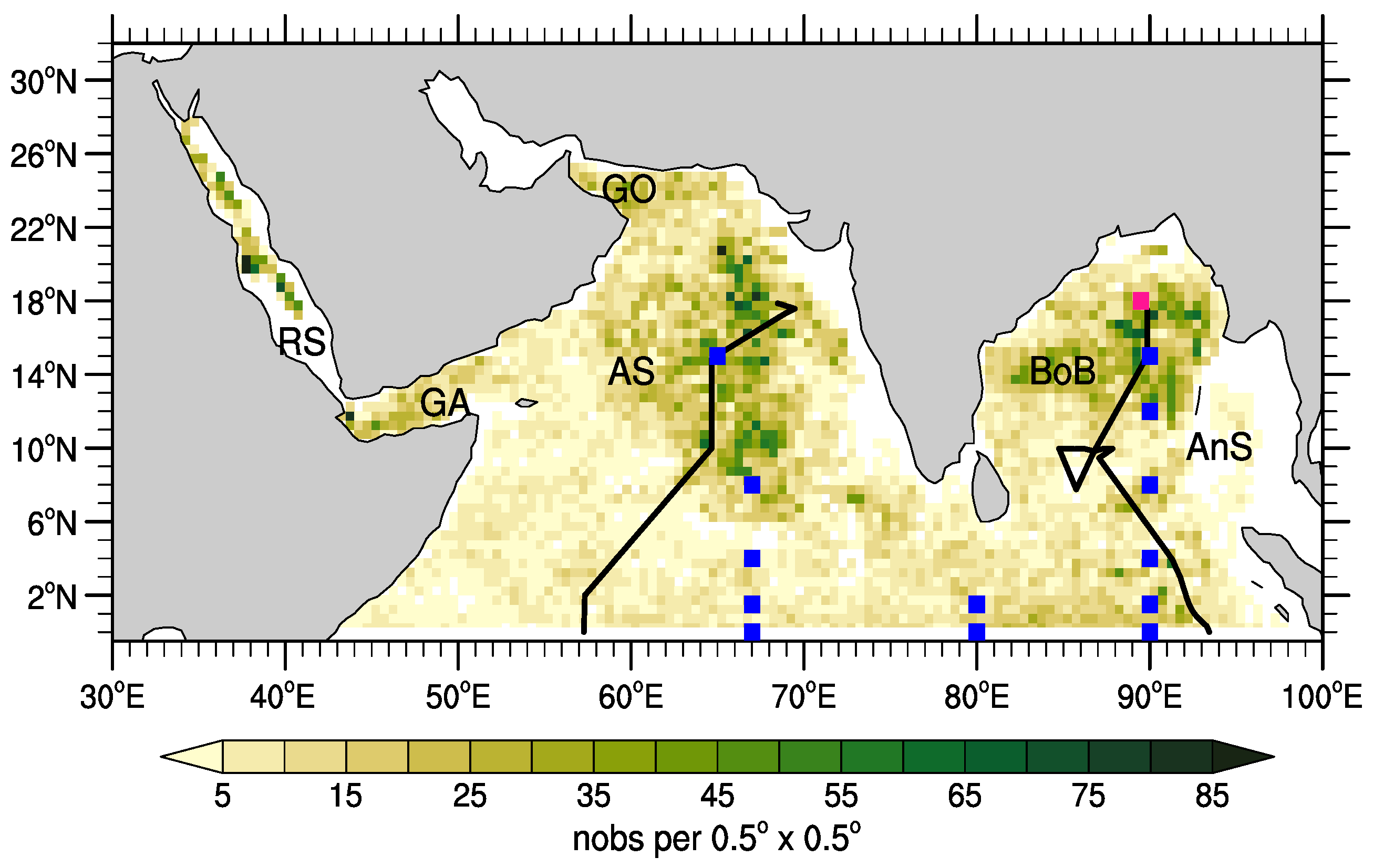
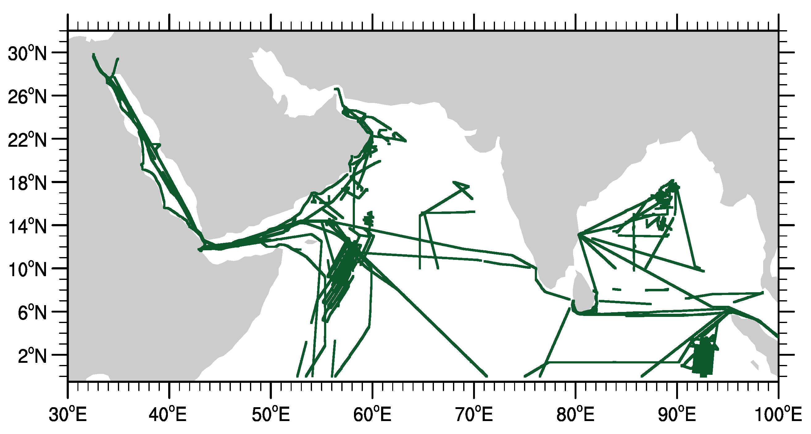
For assessing SMAP SSS, this work uses almost all publicly available in situ salinity measurements over the SMAP era. They come from a variety of sources that include Argo floats, thermosalinographs (TSG), ship-based Conductivity–Salinity–Depth (CTD) from the Global Ocean Ship-based Hydrographic Investigations Program (GO-SHIP) [32], and time series from moored buoys.

Satellite and in situ salinity measurements are inherently different due to technological constraints. Boutin et al. [33] and Vinogradova et al. [4] give excellent overviews of these differences and implications. For instance, SSS from L-band radiometers refers to the first top centimeter of the ocean, while in situ measurements are usually from 1 to 10 meters below the sea surface depending on in situ instrument characteristics. In the case of intense precipitation, salinity near the air–sea interface may be fresher than that in 1-m depth or below. Some in situ observations are instantaneous measurements, such as from Argo floats; others can be hourly or daily averages, such as time series from moored buoys, and these differences may affect comparison statistics between satellite and in situ observations. Moreover, there is variability within the satellite footprint that is captured by in situ measurements but not by the satellite, in which SSS can be interpreted as a spatial-average over the footprint [33,34,35]. Because of the inconsistency between satellite and in situ measurements, the present work uses the term “difference” instead of “error” to refer to it (see [4] for a discussion on this matter).

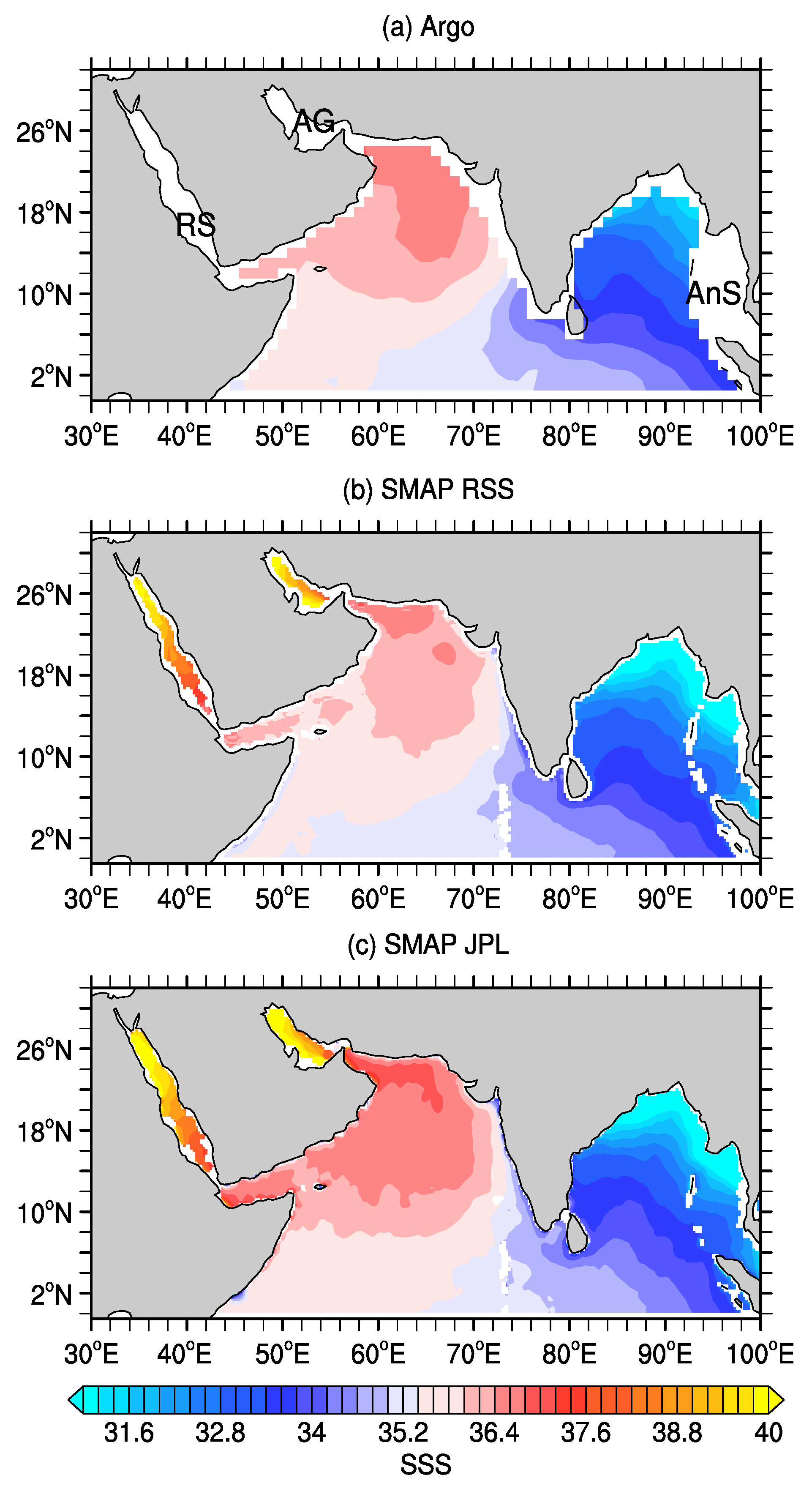
Figure 1 shows the mean SSS field for four years (September 2015 to September 2019) based on Argo in situ observations mapped into a 1°× 1° grid [36], and the mean fields from the two SMAP products that are evaluated in the present work. The period for calculating the mean fields was chosen to start in September 2015 because there was an indication that SMAP SSS retrievals may have been degraded during the early months of the mission (April–August 2015) [6].

In the long-term mean, in situ and satellite fields agree relatively well with a strong east–west gradient of surface salinity: SSS varies from less than 32.4 in the Bay of Bengal to more than 36.6 in the Arabian Sea, although RSS/JPL products slightly under-/overestimated in situ SSS as measured by Argo in the Arabian Sea. Broadly speaking, the Indian Ocean salinity pattern is controlled by four major processes [37,38,39,40,41,42,43]: net-air sea fluxes (evaporation minus precipitation), runoff from large rivers in the Bay of Bengal, inflow of relatively fresh waters from the Pacific Ocean through Indonesian throughflow straits, and inflow of saltier waters from the Red Sea and the Arabian/Persian Gulf. The wide salinity range and a variety of processes controlling SSS make the North Indian Ocean especially attractive to assess spaceborne SSS measurements.

A difference in the maps of Figure 1 is the absence of in situ observations in marginal seas (the Red Sea and the Arabian/Persian Gulf in the western, and the Andaman Sea in the eastern). Marginal seas are usually not included in Argo-gridded products [4,36] because the amount of in situ observations is much reduced and even nonexistent in these regions, such as in the very shallow Arabian/Persian Gulf (maximum depths of 110–160 m [44]). In the SMAP fields of Figure 1, there are also defined SSS values closer to the coast than in the Argo SSS mean-field as float-parking depth is around 1000 m, with few observations in shallow waters (<1000 m) in the standard Argo program [36].

Apart from Argo, other sources of in situ salinity observations are also sparse in time and space in marginal seas of the Indian Ocean. Take, for instance, the extremely salty Red Sea. Most knowledge of salinity dynamics there is based on numerical simulations, and few in situ observations exist [22,45,46,47,48,49,50]. The scarcity of salinity measurements may be surprising because the Red Sea has one of Earth’s largest evaporation rates with an annual mean of around 2 m/yr, which makes the Red Sea a crucial source of moisture for the arid Middle Eastern atmosphere and an essential component of the regional hydrological cycle [46,51,52,53]. In consequence of the extreme evaporation, freshwater must be imported from adjacent basins (the Gulf of Aden and the Arabian Sea) to keep sea level and mean salinity in a steady-state [48]. As part of the ocean dynamics (which is controlled by buoyancy forcing dominated by salinity [54]), one of the saltiest water masses of the global oceans is formed in the extreme north of the Red Sea: the Red Sea Overflow Water (RSOW), which escapes the marginal sea and spreads to the intermediate depths of the whole Indian Ocean [24]. Although salinity is a crucial variable in the Red Sea, both as an indicator of the regional hydrological cycle and as a dynamical forcing, our knowledge about its variability is incipient given the scarcity of in situ observations e.g., [22,51].

Therefore, it is appropriate to ask whether SMAP could capture salinity in a narrow marginal sea such as the Red Sea. It is now known that SMAP can retrieve signals, although with limitations, in complex regions such as the Mediterranean Sea and the Arctic Ocean. However, the maximum Red Sea width is only about 355 km with coastlines on both sides, so land contamination and the RFI may be a severe issue precluding SSS retrievals. A similar problem may occur in the Gulf of Aden that is surrounded by land. The present work addresses this problem through exploratory analysis of SMAP data in these particular areas, and results are promising for the Red Sea.

The paper is organized as follows: Section 2 describes satellite and in situ SSS data, and collocation procedures and statistics used to assess SMAP performance; Section 3 outlines statistical-analysis results for the Arabian Sea (Section 3.1), Bay of Bengal (Section 3.2), and the Red Sea (Section 3.3); Section 4 and Section 5 provide a discussion and a summary of the present work, respectively.

2. Data and Methods

2.1. SMAP Products

This work assesses the latest version of two different SMAP product series in the North Indian Ocean (0°–31°N; 30°–100°E) against in situ SSS observations collected by a variety of instruments in the period of 1 April 2015 to 30 September 2019. Because the goal here was to evaluate SMAP SSS, the early months of the mission (April–August 2015), in which retrievals may have been degraded [6], were included. All SSS observations used in the present work are in the 1978 Practical Salinity Scale (PSS-1978) [55].

One SMAP product series was processed by using the Geophysical Model Function (GMF) for the Combined Active–Passive (CAP) algorithm [3,7,56], and distributed by the NASA/JPL/Physical Oceanography Distributed Active Archive Center (PO.DAAC). Hereafter, we refer to this product series as CAP/JPL. The other SMAP series was produced by RSS using Aquarius version 5.0 GMF adapted to the SMAP mission [2,57]. From now on, this study refers to those SMAP products as RSS. Except for a significant gap between 17 June 2019 and 25 July 2019 when the SMAP satellite was offline due to a spacecraft issue, both series span almost continually from April 2015 to the present, and are composed of Level-2 (L2; along-track data) and Level-3 (L3; global gridded maps) datasets.

Besides distinct GMFs, the RSS and CAP/JPL series also differ in correction schemes and ancillary data used to retrieve SSS. For example, CAP/JPL relies on winds from the National Oceanic and Atmospheric Administration/National Centers for Environmental Prediction (NOAA/NCEP) Global Forecast System (GFS) atmospheric model. The RSS series, on the other hand, uses Cross-Calibrated Multiplatform (CCMP) gridded surface vector winds that are mostly based on satellite microwave winds. The use of distinct wind products is likely to contribute to differences in salinity retrievals between CAP/JPL and RSS in the North Indian Ocean, which is dominated by the South Asian monsoonal wind regime. A full description of processing, ancillary data, and global validation is given by Fore et al. [7] (CAP/JPL) and by Meissner et al. [57] (RSS).

CAP/JPL products used here belong to version 4.2, released on 24 January 2019, and comprise of L2B data distributed on a 25 km swath grid with 1624 × 76 cells (along/cross-track) per satellite revolution and L3 8-day running average fields [7,58]. These L3 fields are available on a uniform 0.25° × 0.25° rectangular grid and have daily time steps. For producing them, L2B data were averaged over the 8-day period (centered at midpoint), and a Gaussian weight function with a search radius of about 45 km and a half-power radius of 30 km was used to map the data into the 0.25° grid. For the CAP/JPL v4.2 datasets, the effective spatial resolution of the SSS fields is about 60 km. Globally, the mean bias of CAP/JPL v4.2 in relation to Argo-gridded products is less than 0.1, with an $rmsd$ of 0.3 [7].

RSS products belong to version 4.0, released on 29 August 2019, and include L2C and L3 8-day running average datasets [6]. For both processing levels, RSS data are distributed in two spatial resolutions: 40 and 70 km. The 70 km data are obtained by smoothing the 40 km product using a simple near-neighbor averaging scheme over 9 cells (8 adjacent and the center cell itself) and should be considered the RSS official product for open-ocean applications. Different from CAP/JPL, in the RSS processing, Level-1 swath data were first interpolated onto a fixed 0.25° Earth grid at approximately 40 km spatial resolution using Backus–Gilbert optimal interpolation that maintains the approximated resolution and shape (39 × 47 km) of the original data (see Meissner et al. [57] for more detail). Consequently, the RSS L2C grid has different dimensions (1526 × 720 cells) than the CAP/JPL L2B. For each location in L2C data, there are SSS retrievals for both fore and aft directions [2]. This format is different from that of L2B CAP/JPL, in which a single salinity retrieval is available per cell. Besides the 1-month data gap in June/July 2019, there are also some other missing L2C data, since salinity is not retrieved in RSS products when there are incomplete ancillary data [57].

The $rmsd$ of L3 RSS-70 km version 3.0 and Argo gridded data was about 0.15 at 1° resolution after August 2015, being slightly higher for the RSS-v3 40 km (around 0.2). No global $rmsd$ estimation for version 4.0 has been released yet. Meissner et al. [57] showed that, during the early months of the SMAP mission (April–August 2015), the $rmsd$ was much higher in version 3 (Figure 21 in [57]), indicating a significant degradation in SMAP SSS. However, the causes are unknown to date.

2.2. In Situ Observations

2.2.1. Argo Floats

For the present work, SSS observations, collected by Argo floats in the North Indian Ocean (0°–31°N; 30°–100°E) for the period of 1 April 2015 to 30 September 2019, were selected from the global CORIOLIS repository (http://www.coriolis.eu.org/) that contains data from all Argo floats deployed to date. This 4-year subset consists of 37,693 measurements (Figure 2) after the quality-control (QC) procedure described below, and includes both delayed-mode and real-time data from 320 individual floats. About 12% of the original measurements were rejected in the QC.

From the original subset, only floats with valid salinity measurements between the sea surface and 10 m depth were selected. For each float (time, position), SSS refers to the nearest sea-surface depth. In the 4-year QC subset, about 42.6% of SSS measurements were collected between 2 and 5 m depth, 30.1% between 5 and 10 m, and 27.3% were shallower than 2 m. The seasonal distribution of SSS measurements is relatively homogeneous in the North Indian Ocean as a whole: June holds a maximum number of observations with 10.5% of the total, and November the minimum (7%). For comparison with SMAP data, we gave preference for delayed mode or adjusted values. Only SSS measurements with quality-control flag issued as 1 or 2 (good or probably good) for position, time, pressure, and salinity, were selected, and duplicate data were discarded.

Moreover, 53 floats in which salinity or pressure sensors were flagged in the Argo gray list were not used for comparison with SMAP over the flagged period except for the Red Sea. From the 6 Argo floats there, 4 floats (1900959, 1900960, 1901521, 6900425) belong to the Seabird CTD batch (6000–7100) that may develop a high salinity bias within 2 years of deployment. In situ SSS observations are scarce in the Red Sea, and because of that, these Argo floats were used for statistical analysis. The complete Argo float gray list can be found at https://www.nodc.noaa.gov/argo/grey_floats.htm (or at ftp://ftp.ifremer.fr/ifremer/argo/ar_greylist.txt). A visual screening was also used to eliminate clear outliers in Argo measurements that occurred in near real-time data.

2.2.2. Thermosalinograph (TSG)

All TSG observations in the North Indian Ocean between 1 April 2015 and 30 September 2019 were downloaded from the CORIOLIS repository that also distributed data from the Global Ocean Surface Underway Data (GOSUD) Project. The CORIOLIS/GOSUD dataset consists of SSS observations collected by 6 different platforms (

Table 1. Thermosalinograph (TSG) SSS observations used to assess SMAP performance in North Indian Ocean (0°–31°N; 30°–100°E). Year indicates when the ship visited North Indian Ocean; Depth is TSG nominal depth, Coverage shows zonal extension covered by cruises, and N is the number of valid observations collected by each platform between 1 April 2015 and 30 September 2019. Data in 1–6 obtained from the CORIOLIS website, and in 7–10 from National Oceanic and Atmospheric Administration/National Centers for Environmental Information (NOAA/NCEI) TSG Data Portal. NOAA/NCEI TSG data distributed with a temporal resolution of 1 min; CORIOLIS, about 2–5 min.

	Platform	Year	Depth (m)	Coverage	N
1	9VBM5 (CMA CGM Onyx)	2015 2016	9.0	32°E–100°E	19,500
2	FABB (R/V Beautemps-Beaupré SHOM a)	2017 2019	3.5	32°E–63°E	13,018
3	FLES (Fleur Australe)	2017	1.0	32°E–60°E	2121
4	FMCY (R/V Pourquoi-Pas? IFREMER b)	2015	5.3	33°E–55°E	8483
5	FNIN (R/V Marion Dufresne IPEV c)	2016 2017	6.0	75°E–95°E	29,705
6	FNUR (R/V Antea IRD d)	2016	1.6	32°E–60°E	7837
7	KAOU (R/V Roger Revelle SIO e)	2015 2016	5.0	80°E–93°E	50,935
8	WSAF (R/V Sally Ride SIO)	2019	3.5	80°E–100°E	70,614
9	KTDQ (R/V Thomas G. Thompson UW f)	2018	4.0	84°E–90°E	20,731
10	WTEC (NOAA Ship Ronald H. Brown)	2018	5.3	64°E–70°E	13,808

${}^{\mathrm{a}}$ Service Hydrographique et Océanographique de la Marine; ${}^{\mathrm{b}}$ Institut Français de Recherche pour l’exploitation de la Mer; ${}^{\mathrm{c}}$ Institut Polaire Français Paul-Émile Victor; ${}^{\mathrm{d}}$ Institut de Recherche pour le Développement; ${}^{\mathrm{e}}$ Scripps Institution of Oceanography; ${}^{\mathrm{f}}$ University of Washington.

). However, this dataset lacks TSG data collected by U.S. research vessels that are available at the NOAA National Centers for Environmental Information (NOAA/NCEI) TSG portal. Thus, we augmented the original CORIOLIS/GOSUD dataset with NOAA/NCEI TSG data to have comprehensive TSG salinity data (Table 1). Before merging the 2 datasets, the respective quality-control flags were individually applied to each file, and only observations classified as of good or probably good quality were selected, totaling 236,750 samples. The nominal depth of TSG intake water varies from ship to ship; in our set, it went from 1.6 to 9 m. These SSS along-track observations have a spatial resolution of about 1–3 km and were taken under different years. About 26.8% of TSG measurements were obtained in 2015, 17.2% in 2016, 7.3% in 2017, 14.6% in 2018, and 34.1% in 2019. Seasonally, 51% of all observations were taken in summer (June–July, boreal seasons hereafter), while only 6% in winter (December-March). The spatial distribution of TSG data in the North Indian Ocean is also much more heterogeneous than that from Argo floats, with large areas without any observation (Figure 3).

2.2.3. Moored Buoys

Daily-average time series of surface salinity from 13 Research Moored Array for African–Asian–Australian Monsoon Analysis and Prediction (RAMA) buoys located north of the equator (Figure 2) were downloaded from the Tropical Atmosphere Ocean project, Pacific Marine Laboratory (TAO/PMEL) website [59]. Only salinity observations from the first 2 depth levels (1 and 5 or 10 m) with quality-control flag issued as good were used. Six moorings are located in the equatorial zone at (0°–1.5°N), 3 in the Arabian Sea (4°–15°N, 65°–67°E), and 4 in the Bay of Bengal (4°–15°N, 90°E) (Figure 2). From the 13 buoys, only 4 spanned the 4 years of SMAP operation (

Table 2. Research Moored Array for African–Asian–Australian Monsoon Analysis and Prediction (RAMA) daily salinity observations over the SMAP era (1 April 2015 to 30 September 2019). First column shows the mooring location. Second/third columns indicate mooring start/end time (if the cell is empty, mooring is still operational as of 1 October 2019). Fourth and fifth columns show the percentage of valid in situ observations at sea surface (1 m) and subsurface (5 or 10 m depth) between 1 April 2015 (or buoy start time, which is recent) and 30 September 2019 (or end time for nonoperational buoys).

Mooring	Start	End	Surface	Subsurface
0.0°N 67.0°E *	7 July 2014		78.33	64.70 [10 m]
0.0°N 80.5°E *	23 October 2004		50.94	0.0 [5 m]
0.0°N 90.0°E	9 November 2004	28 September 2018	56.74	70.30 [10 m]
1.5°N 67.0°E	15 August 2017		30.65	68.99 [10 m]
1.5°N 80.5°E	21 October 2004	26 October 2015	28.36	28.36 [10 m]
1.5°N 90.0°E	17 September 2006	10 March 2016	30.52	28.20 [10 m]
4.0°N 67.0°E	27 June 2018		55.00	94.56 [10 m]
4.0°N 90.0°E	16 November 2006	31 July 2018	41.00	25.80 [10 m]
8.0°N 67.0°E	22 June 2018		45.38	73.76 [10 m]
8.0°N 90.0°E *	15 November 2006	19 August 2019	44.10	58.21 [10 m]
12.0°N 90.0°E *	16 November 2007		76.20	89.10 [10 m]
15.0°N 65.0°E	19 June 2018	11 November 2018	78.62	96.55 [5 m]
15.0°N 90.0°E	17 November 2007	22 July 2018	60.60	53.56 [10 m]

* Buoys span four years of SMAP operation.

). Even in the overlapping period between SMAP and in situ observations, some buoys returned few valid measurements, such as the 2 buoys at 1.5°E, east of 80°(about 30% for both surface and subsurface sensors; Table 2). As there were few observations in both depths, these 2 buoys were not used in the comparison with SMAP.

Besides observations from the RAMA array, we also used SSS observations at a nominal depth of 1 m from the WHOI Bay of Bengal Mooring at 18°N–89.5°E (Figure 2). The WHOI mooring [60] worked from 9 December 2014 to 29 January 2016, overlapping for 10 months with SMAP. Surface data, including meteorological parameters, are available at the WHOI Upper Ocean Process Group website (http://uop.whoi.edu/projects/Bengal/QCData.html), with resolutions of 1 min, hourly, and daily averages. All data were quality-controlled by the WHOI group. For comparison with SMAP, this study used the daily averages. Different from the RAMA buoys, the WHOI SSS time series is almost complete.

2.2.4. Ship-Based CTD

Over the SMAP era (April 2015–September 2019), 2 meridional transects were occupied in the North Indian Ocean as part of the international GO-SHIP program [32] (Figure 2). One transect was in the Arabian Sea (2018) and is known as the I07N line. The second transect was in the Bay of Bengal (2016) and is known as the I09N.

In the Arabian Sea, the northern portion of I07N extended from the equator to 18°N and took place between 22 May 2018 and 4 June 2018. SSS observations were collected in a total of 48 stations, spaced 50 km apart on average. In the Bay of Bengal, the northern portion of the I09N (0°N–18°N) was occupied in 10–24 April 2016 in a total of 57 stations (also spaced 50 km apart in average). For both transects, SSS was collected using ship-based CTD instruments and it refers to salinity at 2 to 5 dbar. In the GO-SHIP, CTD salinity observations were calibrated against in situ samples from Niskin bottles, which were measured using Guildline 8400 Austosal salinometers, calibrated using the International Association for the Physical Sciences of the Oceans (IAPSO) Standard Sea Waters (SSW). GO-SHIP salinity observations are of the highest quality and aim for climate studies. Data are publicly available at the CLIVAR Carbon Hydrographic Data Office (CCHDO) website.

2.3. Collocation between SMAP and In Situ Observations and Statistics

For assessing several SMAP products, pairs of concurrent SMAP and in situ observations (Argo, TSG, moored buoys, and ship-based CTD) were first formed by selecting satellite data from the closest grid cell to in situ observations (details are given below in the respective subsections). Currently, there is no consensus in the community about the best methodology and a single criterion to do the match up because in situ and satellite SSS observations are intrinsically different. Any criterion is ad hoc. Here, this task was performed individually for each of the 6 SMAP products that were assessed: 8 day running average L3 (CAP/JPL, RSS-40 km, and RSS-70 km) and L2 (CAP/JPL, RSS-40 km, and RSS-70 km). No space–time interpolation was performed for SMAP data. This study refers to these data pairs (SMAP, in-situ) as collocated observations. These pairs, however, are not strictly collocated because of the intrinsic differences between satellite and in situ observations [4,33,34].

Basic statistics such as the linear correlation coefficient, $rmsd$$\left(\sqrt{{\displaystyle \frac{1}{N}}{\sum }_{i=1}^N{(x_i-y_i)}^2}\right)$, bias, and histograms were calculated for each SMAP product for the collocated datasets to assess SMAP performance in the North Indian Ocean in both the spatial and temporal domains. These statistics are generally used in studies evaluating satellite salinity observations [1,3,8,9,12,13,16,17,18,21,61].

2.3.1. Argo Collocation Procedure

For the L3 datasets, the following steps were performed. First, for each Argo observation, SSS${}_{argo}$ (t,x,y), the SMAP field correspondent to day t was selected; then, the salinity value at the grid cell in which the in situ observation resided (x,y) was extracted. L3 daily fields are averages, centered at the midpoint over an 8-day interval; therefore, the comparison is between measurements that are not quite equivalent (Argo floats give instantaneous measurements).

For the L3 RSS-40 km product, a total of 36,285 collocated pairs were formed in the North Indian Ocean, 36,068 for the RSS-70 km, and 36,553 for CAP/JPL. These collocated subsets excluded pairs in which salinity difference between SMAP and Argo was larger than 2, which was less than 0.5% of the total. For example, from the 36,197 original L3 RSS-70 km pairs, only 129 had salinity differences larger than 2. These pairs were labeled as outliers and discarded as these differences might be due to Argo errors because a large portion of Argo data in the North Indian Ocean have only passed through automatic near-real-time QC checking. In the collocated L3 pairs, the median distance between the SMAP grid cell center and Argo float positions was about 11 km.

For the L2 products, a slightly different match-up procedure was adopted. The aim was to have data pairs that were obtained as close in both time and space as possible. For that, for each in situ SSS${}_{argo}$ (t,x,y), the algorithm selected the SMAP value from the closet grid cell to the in situ position on a radius of 25 km, taken up to $\pm 12$ h from the in situ observation. For RSS products, the ancillary 32-bit quality-control flag —available in the L2C files —was used to discard strongly degraded SMAP measurements [57] (pp. 37, 39). Besides these QC checks, L2C data with rain flags were also discarded. For comparison with in situ observations, valid fore and aft data, which were taken minutes apart, were averaged. Only collocated observations that had both the 40 and 70 km salinity retrievals were considered. For L2B CAP/JPL, the ancillary 16-bit quality-control variable was used to discard SMAP salinity retrievals that were not of good quality [7] (Section 6.2.24). Collocated observations in which salinity differences between L2 and in situ data were above 2 were also discarded for statistical comparisons (136 data pairs for RSS and 120 for the CAP/JPL).

A total of 11,378 collocated pairs were formed for the RSS L2C data, and 13,475 for the L2B CAP/JPL. In these pairs, the median distance between SMAP grid cell center and Argo float positions was about 11.3 km (RSS) and 9.5 km (CAP/JPL), and 5.6 h for both. Note that, for the CAP/JPL, many L2B files for 2015 had the row_time variable (approximate observation time for each swath row) with month/year that did not match the filename timestamp. For safety’s sake, these files were discarded and not used for comparison with in situ data.

2.3.2. TSG Collocation Procedure

Unlike Argo observations, TSG data are collected along the ship tracks with a high spatial resolution of 1 to 3 km (Figure 3), which results in a substantial number of samples. The following steps were performed to match up satellite and TSG observations; the aim was both to avoid oversampling bias and to smooth submesoscale variability present in TSG observations. For the L3 products, for each day t that TSG observations existed, the respective SMAP field was selected. Then, SSS${}_{TSG}$ from day t was spatially averaged over SMAP grid cells ($i,j$). Then, for each grid cell ($i,j$) in which SMAP and TSG data were valid, the pair was formed as [SMAP$(t,i,j)$ $\langle \mathrm{TSG}\rangle \left(t\right)$]. For SMAP data, no interpolation/smoothing was performed. Following this procedure, a total of 5,116 collocated pairs were formed for the L3 RSS-40 km product over the North Indian Ocean; 4,946 for RSS-70 km, and 5199 for CAP/JPL.

A similar procedure to that described above was used for matching up the TSG to L2 data except that the SMAP data had to be no more than $\pm 12$ h apart from the averaged grid-cell TSG observation. Similar to the Argo case, only QC SMAP data was used, and the fore and aft data were averaged for the RSS product. A total of 2340 (40 km) and 2307 (70 km) pairs were formed for the L2C RSS product and 1908 for the L2B CAP/JPL. The time-mean difference between the observations in these collocated datasets is about six hours. Note that the number of collocated observations is much less for the CAP/JPL product because the files from 2015 were not used (see the previous section), and many of the TSG observations are from this year (Table 1). In various TSG collocated observations, there is a large number of pairs with salinity differences above 2 (3–10%). Thus, these pairs cannot be considered outliers and were kept for the statistical analysis, unless otherwise stated.

2.3.3. Collocation Procedure for Moored-Buoy Time Series and Ship-Based CTD

For in situ observations from buoys and ship-based CTDs, only comparisons with L3 SMAP products were performed, since these in situ data were much fewer and more scattered in space and time than those of the Argo and TSG datasets. For the buoys, the SMAP SSS time series from the grid cells at the buoy locations were extracted. For ship-based CTDs, for each SSS${}_{CTD}(t,x,y)$ in situ observation, the salinity value from the grid cell in which the in situ observation resided (x,y) was extracted for same day t as that in the in situ data.

3. Results

In the present work, the 80°E meridian was used to delimit the salty western from the much fresher eastern (Figure 1). The western side encompasses the Arabian Sea, the Gulfs of Aden and Oman, and the Red Sea and the Arabian/Persian Gulf. The eastern side includes the Bay of Bengal and the Andaman Sea. Because there are no in situ SSS observations in the Arabian/Persian Gulf over the SMAP era in public repositories such as CORIOLIS, GOSUD, or NCEI (see Figure 2 and Figure 3), this study did not perform a statistical evaluation there.

This section starts by assessing SMAP salinity in the Arabian Sea, the Bay of Bengal, and their surroundings. A comparison with the Red Sea is made in a dedicated section since the Red Sea is a challenging region for salinity remote sensing. For the Red Sea, the analysis is exploratory and based on TSG data besides the six Argo floats.

3.1. Arabian Sea

From all collocated SMAP and Argo observations, around 60% are located west of the 80°E (excluding the Red Sea), which this study refers to as the Arabian Sea for short (although it also encompasses the near-equatorial area, and the Gulfs of Aden and Oman). About half of the collocated Argo observations were taken between 2 and 5 m depth (

Table 3. Comparison of collocated SSS from SMAP and Argo observations in Arabian Sea (0°–31°N; 30°–80°E, excluding Red Sea) between 1 April 2015 and 30 September 2019. Upper part: number N of collocated observations over considered period, number of individual Argo floats, and vertical distribution of Argo observations in relation to total of collocated data in the region. Middle part: statistics (mean, maximum, minimum, standard deviation, and skewness) for each individual dataset (values between brackets are for Argo, and outside for SMAP). Lower part: statistics of collocated observations. $correl$: linear correlation coefficients that were significantly different from zero at 95% confidence (p-value); $\Delta$: differences between SMAP and Argo observations (SMAP − Argo); $bias$: mean difference ($bias=\overline{\Delta }$); $rmsd$: root mean square difference; $skew(\Delta )$: skewness of probability distribution of the differences. Values between parenthesis in Level 2 columns are for RSS-L2C 40 km product; between brackets are for Argo.

		Level 3			Level 2
		RSS-40 km	RSS-70 km	CAP/JPL	RSS	CAP/JPL
	N	21,877	21,702	22,035	7776	9158
	floats	218	216	219	212	200
	<2 m	26.48%	26.57%	26.29%	24.45%	26.23%
	2–5 m	44.83%	44.59%	45.10%	43.93%	44.99%
	5–10 m	28.68%	28.83%	28.61%	31.62%	28.78%
	mean	35.81 [36.00]	35.82 [36.00]	36.20 [36.01]	35.91 [36.08] (35.91)	36.26 [36.07]
	max	39.12 [37.81]	37.82 [37.81]	38.67 [37.81]	38.29 [37.32] (38.93)	38.95 [37.81]
	min	31.20 [31.48]	31.19 [31.48]	31.55 [31.48]	31.96 [31.70] (31.63)	31.85 [31.70]
	std	0.74 [0.73]	0.68 [0.73]	0.75 [0.73]	0.69 [0.69] (0.82)	0.88 [0.69]
	skew	−0.75 [−1.09]	−1.04 [−1.09]	−0.90 [−1.10]	−0.84 [−1.27] (−0.41)	−0.50 [−1.26]
	$correl$	0.88	0.94	0.92	0.86 (0.74)	0.71
	p-value	<0.001	<0.001	<0.001	<0.001 (<0.001)	<0.001
	$bias$	−0.19	−0.18	0.20	−0.17 (−0.17)	0.19
	$rmsd$	0.41	0.31	0.36	0.40 (0.59)	0.62
	$skew(\Delta )$	−0.18	−0.19	0.36	0.06 (0.07)	0.04

), and their temporal distribution is relatively homogeneous, with all seasons well-represented. Spatially, Argo data density is higher in the eastern side of the Arabian Sea, with 80–85 observations per 0.5° grid cell over four years (Figure 2). In the region west of 60°E, Argo data density was, on average, much lower.

Overall, all products reproduce Argo SSS observations in the Arabian Sea relatively well (Figure 4). Correlation coefficients vary from 0.71 (L2B CAP/JPL) to 0.94 (L3 RSS-70 km), with statistics improving with the smoothing of SMAP data in space and time (Table 3). For instance, for L3 products, correlation increases, and $rmsd$ decreases with spatial smoothing, such that CAP/JPL (60 km) has better performance than RSS-40 km but worse than RSS-70 km. A similar improvement is observed when SMAP data is averaged in time, with correlation being lower and $rmsd$ higher for L2 products when contrasted with the respective L3 data (Table 3). For example, RSS-40 km data have an $rmsd$ of 0.41 for L3, but 0.59 for L2. Scatter plots in Figure 4 also show that SMAP products with less smoothing (L2 and L3 RSS-40 km) have high salinity values that were not observed by Argo.

Basic statistics of SSS distributions —mean, minimum, standard deviation, and skewness —are similar for different datasets (Table 3, middle), with all of them presenting moderate–high, left-tailed skewed distribution (long tail in low salinity values). Statistical distributions from Argo data, however, tend to be slightly more skewed than those from SMAP products.

Similar conclusions can be reached when looking at collocated SMAP–TSG (

Table 4. Comparison of collocated SSS SMAP and TSG observations in the Arabian Sea (0°–31°N; 30°–80°E, excluding Red Sea) between 1 April 2015, and 30 September 2019. The same statistics as shown in Table 3. Values between brackets are for TSG, and between parenthesis in Level 2 columns are for RSS-L2C 40 km product.

		Level 3			Level 2
		RSS-40 km	RSS 70 km	CAP/JPL	RSS	CAP/JPL
	N	2630	2599	2697	1161 (1172)	998
	mean	35.85 [35.98]	35.85 [35.98]	36.21 [35.99]	35.90 [36.03] (35.89)	36.27 [36.01]
	max	38.21 [37.18]	38.11 [36.99]	38.19 [37.34]	38.55 [36.96] (39.22)	38.60 [36.96]
	min	32.96 [34.15]	33.80 [34.28]	32.84 [33.56]	33.17 [34.32] (32.36)	33.61 [34.28]
	std	0.64 [0.51]	0.54 [0.51]	0.62 [0.52]	0.61 [0.47] (0.85)	0.79 [0.45]
	skew	−0.29 [−0.82]	−0.50 [−0.81]	−0.72 [−0.84]	−0.05 [−0.89] (0.01)	−0.11 [−0.96]
	$correl$	0.75	0.86	0.85	0.68 (0.52)	0.65
	p-value	<0.001	<0.001	<0.001	<0.001 (<0.001)	<0.001
	$bias$	−0.13	−0.12	0.22	−0.14 (−0.14)	0.27
	$rmsd$	0.44	0.31	0.37	0.47 (0.74)	0.66
	$skew(\Delta )$	−0.47	−0.13	−0.20	−0.07 (−0.31)	0.16

) or SMAP-RAMA (

Table 5. Comparison of SSS observations from SMAP and RAMA array buoys (daily averages) at 1 m and at subsurface (5 or 10 m; see Table 2) in the Arabian Sea between 1 April 2015 (or buoy start time, which is recent) and 30 September 2019 (or end time for nonoperational buoys). The same statistics as shown in Table 3. Values between brackets relative to subsurface in situ observations, and outside brackets at 1 m depth. Linear correlation coefficients were significantly different from zero at 95% confidence (p-value < 0.001).

		Level 3
		RSS-40 km	RSS 70 km	CAP/JPL
$correl$	0.0°N 67.0°E	0.79 [0.76]	0.85 [0.85]	0.76 [0.75]
	1.5°N 67.0°E	0.84 [0.70]	0.89 [0.79]	0.84 [0.69]
	4.0°N 67.0°E	0.89 [0.91]	0.92 [0.93]	0.88 [0.89]
	8.0°N 67.0°E	0.79 [0.92]	0.90 [0.95]	0.89 [0.95]
	15.0°N 65.0°E	0.67 [0.69]	0.64 [0.70]	0.82 [0.85]
$bias$	0.0°N 67.0°E	−0.01 [−0.12]	−0.04 [−0.11]	0.15 [0.07]
	1.5°N 67.0°E	−0.04 [0.06]	−0.06 [0.06]	0.17 [0.29]
	4.0°N 67.0°E	0.06 [−0.07]	−0.04 [−0.12]	0.28 [0.18]
	8.0°N 67.0°E	−0.11 [−0.13]	−0.11 [−0.12]	0.27 [0.24]
	15.0°N 65.0°E	−0.25 [−0.27]	−0.30 [−0.31]	0.30 [0.24]
$rmsd$	0.0°N 67.0°E	0.26 [0.29]	0.20 [0.22]	0.30 [0.26]
	1.5°N 67.0°E	0.27 [0.37]	0.19 [0.29]	0.28 [0.46]
	4.0°N 67.0°E	0.28 [0.27]	0.23 [0.21]	0.41 [0.35]
	8.0°N 67.0°E	0.32 [0.33]	0.20 [0.24]	0.34 [0.35]
	15.0°N 65.0°E	0.37 [0.36]	0.22 [0.18]	0.38 [0.35]
$skew(\Delta$)	0.0°N 67.0°E	−0.37 [−0.37]	−0.85 [−0.77]	−0.51 [−0.46]
	1.5°N 67.0°E	−0.24 [0.27]	−0.52 [0.50]	−0.38 [0.37]
	4.0°N 67.0°E	−0.45 [−0.24]	−0.08 [−0.07]	−0.09 [−0.08]
	8.0°N 67.0°E	−0.94 [−0.95]	−0.36 [−0.42]	−0.45 [−0.77]
	15.0°N 65.0°E	0.17 [0.13]	0.74 [−0.25]	0.71 [0.53]
N	0.0°N 67.0°E	1288 [1065]	1288 [1065]	1284 [1043]
	1.5°N 67.0°E	343 [773]	343 [773]	343 [747]
	4.0°N 67.0°E	253 [436]	253 [436]	252 [410]
	8.0°N 67.0°E	211 [343]	211 [343]	211 [343]
	15.0°N 65.0°E	115 [141]	115 [141]	115 [141]

) datasets. This agreement is despite TSG observations being concentrated closer to the Arabian Peninsula coastline (and not well-distributed seasonally), and RAMA buoy array is located in the eastern Arabian Sea. In general, correlations for the SMAP–TSG datasets (0.52–0.82) are worse than those for SMAP–Argo (0.71–0.94), but $rmsd$ is mostly of the same order (0.3–0.4 for L3 products). In comparison with RAMA buoys, the correlations of several collocated SMAP–RAMA datasets (for both surface and subsurface in situ observations) are in agreement (0.64–0.95) with the ones found for the SMAP-Argo, but the $rmsd$ (0.2–0.4) are overall lower (Table 5).

SMAP also captures well SSS spatial variability during the GO-SHIP I07N cruise in 2018 (Figure 5a), which has a similar resolution (≈ 50 km) to the satellite. Salinity steadily increases northward from the equatorial zone to the heart of the Arabian Sea in both the in situ and the L3 dataset. However, SMAP not only captures this basin-scale pattern, but also mesoscale salinity peaks and troughs observed in GO-SHIP (gray shadings in Figure 5a). Bias is negligible for CAP/JPL, but it is negative for both RSS products (

Table 6. Comparison of collocated SSS Level-3 SMAP and GO-SHIP data for 2018 I07N cruise in the Arabian Sea, and for 2016 I09N in the Bay of Bengal. Statistics similar to Table 3.

		Level 3
		RSS-40 km	RSS 70 km	CAP/JPL
I07N	$correl$	0.85	0.93	0.94
	p-value	<0.001	<0.001	<0.001
	$bias$	−0.25	−0.26	0
	$rmsd$	0.39	0.34	0.20
	$skew(\Delta )$	−0.43	−0.73	−0.40
I09N	$correl$	0.82	0.86	0.83
	p-value	<0.001	<0.001	<0.001
	$bias$	−0.17	−0.18	0.29
	$rmsd$	0.42	0.36	0.44
	$skew(\Delta )$	−0.07	−0.39	−0.61

)— there is an apparent offset, albeit small, in the RSS curves in Figure 5a, especially between 8° and 15° N.

Despite the negligible bias, CAP/JPL is saltier than GO-SHIP from 4° to 8°N (Figure 5a). Correlations are high, as expected, in GO-SHIP (0.85–0.94) as GO-SHIP only samples open-ocean waters. The $rmsd$, however, is of the same order as for the other analyzed datasets here (0.20–0.39).

In conclusion, RSS and CAP/JPL products compare similarly well with Argo, TSG, RAMA, and GO-SHIP observations in the Arabian Sea. Overall, RSS has slightly better skills in the Arabian Sea (higher correlation and lower $rmsd$) compared with similar CAP/JPL products, but these skill differences may not be statistically significant. Indeed, for GO-SHIP, CAP/JPL presents better statistics (Table 6).

However, a crucial difference exists between the two product series. While for all RSS datasets, the bias ($\overline{\Delta }$) is negative in relation to Argo, TSG, GO-SHIP, and almost all RAMA buoy data, in CAP/JPL products, bias is of the same strength but positive (Table 3, Table 4 and Table 5). This indicates that salinity from RSS products is typically fresher than that from in situ observations, while saltier in CAP/JPL. This pattern can also be seen, for example, in the scatterplot between SMAP and Argo shown in Figure 4—most data pairs fell to the right of the 1:1 line in RSS products and left in CAP/JPL.

Freshening/salting satellite bias is not restricted to the Arabian Sea, a particular processing level, or in situ observation type. They are consistent between the L2 and L3 datasets, and found both in the western and eastern basins, although they are larger in L2 products (Figure 6).

If SMAP–Argo salinity differences, shown in Figure 6a,b, for instance, are averaged over boxes of 5° × 5°, RSS freshening bias is more prominent in the eastern Arabian Sea and the western side of the Bay of Bengal (Figure 7). In the equatorial zone and the eastern Bay of Bengal, the RSS bias is less prominent. In general, CAP/JPL bias is more homogeneous in terms of spatial distribution than that of RSS, although CAP/JPL salting is higher in the western Arabian Sea and lower in the eastern.

Spatially, correlations and $rmsd$ between SMAP and Argo have a defined pattern in both RSS and CAP/JPL products (Figure 8). Mainly, correlation increases and $rmsd$ decreases from west to east within the Arabian Sea. This pattern is observed in all six products evaluated here, although Figure 8 only shows two products (L3 RSS-70 km and CAP/JPL) for the sake of clarity. In the western Arabian Sea, performance is slightly better for the L3 RSS-70 km product when compared with L3 CAP/JPL. Thus, most TSG data are located in the region of lower agreement (western Arabian Sea), while the RAMA array is in the higher agreement area (eastern). Therefore, comparison statistics are shown in Table 4 (TSG) and Table 5 (RAMA) reflect that.

SMAP performance in the Gulf of Aden (10°–15°N, west of 51°E) when compared with Argo is worse than that in open-ocean waters, as expected. Correlation is relatively low in L3 CAP/JPL (around 0.4–0.5), and slightly higher (0.4–0.65) for L3 RSS-70 km; $rmsd$ varies from 0.4–0.5 (CAP/JPL) to 0.25–0.4 (RSS-70 km; Figure 8).

To determine the overall SMAP skill in the Gulf of Aden, the collocated Argo and TSG data were merged into two single datasets, one for L3 CAP/JPL and the other for L3 RSS-70 km, and statistics were recalculated. A total of 1260 (RSS) and 1447 (CAP/JPL) pairs were formed for the area between 10°–15°N and 43.5°–51°E. When both Argo and TSG observations are considered together, bias follows the same pattern as before: the RSS product underestimates SSS by 0.11, and CAP/JPL overestimates by 0.37. In this comparison, the $rmsd$ is lower for CAP/JPL (0.35 versus 0.55 for RSS), but correlations are similar for both SMAP products (0.42 and 0.43 for RSS).

Although SMAP L3 SSS time series are generally noisier than RAMA salinity observations in the Arabian Sea, SMAP captures overall seasonal and subseasonal variability in buoy locations south of 15°N (Figure 9). However, SMAP sometimes does not capture the intensity of salinity drops in the equatorial zone, for instance, in January–March 2019 at the 1.5°–67°N buoy. The buoy measured a much stronger freshening than those observed by the satellite (Figure 9d). For the 15°N–65°E mooring, in situ time series was short and with many gaps, and was not shown in Figure 9 for the sake of clarity.

In order to evaluate seasonal SMAP performance, statistics (correlation, biases, and $rmsd$) were calculated in a monthly base using collocated Argo datasets, which constitutes the largest dataset in the Arabian Sea. In this case, all year round, bias is negative for RSS products and positive for CAP/JPL (not shown), confirming the previous analysis. The RSS-70 km product also has slightly better skill than the CAP/JPL and the RSS-40 km products —higher correlations and lower $rmsd$, but CAP/JPL is better than RSS-40 km (Figure 10a).

Figure 10a only shows monthly correlation and $rmsd$ for the L3 datasets, but the plot is similar for L2 products, except that correlation coefficients are lower and $rmsd$ is higher than those of the L3. For all products, correlation in the Arabian Sea tends to be slightly lower in the second half of the year, especially for RSS-40 km that has a well-defined minimum in October. This pattern is also clearly observed in the L2 products (not shown).

3.2. Bay of Bengal

In the region east of 80°E, the seasonal distribution of Argo floats is not as homogeneous as west of that meridian. There are almost double the collocated Argo measurements in June during the wet summer monsoon (about 13% of the total) than in November (7%). Spatially, data density is higher in the interior of the Bay of Bengal than in the equatorial region (Figure 2). Fewer observations exist in the Andaman Sea (92°–100°E). For simplicity, this study refers to the region east of 80°E as the Bay of Bengal, although it also includes the equatorial zone and the Andaman Sea.

The Bay of Bengal is much fresher than the Arabian Sea in both satellite and Argo observations. Minimal salinity in Argo is around 21–22, which is well-captured by all SMAP products (

Table 7. Comparison of collocated SSS SMAP and Argo observations in the Bay of Bengal (0°–31°N; 80°–100°E) between 1 April 2015 and 30 September 2019. Statistics are the same as shown in Table 3. Values between brackets, Argo; between parentheses, RSS-L2C 40 km.

		Level 3			Level 2
		RSS-40 km	RSS-70 km	CAP/JPL	RSS	CAP/JPL
	pairs	13,137	13,130	13,168	2966	3863
	floats	133	133	133	127	124
	<2 m	39.46%	39.43 %	39.36%	35.50%	37.82%
	2–5 m	32.82%	32.82%	32.83%	32.06%	31.30%
	5–10 m	27.72%	27.75%	27.81%	32.43%	30.88%
	mean	33.04 [33.11]	33.04 [33.11]	33.32 [33.11]	33.10 [33.14] (33.11)	33.40 [33.16]
	max	35.85 [35.85]	35.56 [35.85]	35.91 [35.85]	36.05 [35.59] (36.44)	36.86 [35.63]
	min	21.15 [21.42]	21.86 [21.42]	22.09 [21.42]	23.33 [22.38] (23.78)	23.65 [22.38]
	std	1.26 [1.22]	1.23 [1.21]	1.22 [1.21]	1.26 [1.21] (1.31)	1.39 [1.26]
	skew	−1.55 [−1.51]	−1.55 [−1.46]	−1.62 [−1.43]	−1.14 [−1.36] (−0.99)	−1.35 [−1.62]
	$correl$	0.95	0.96	0.95	0.95 (0.91)	0.89
	p−value	<0.001	<0.001	<0.001	<0.001 (<0.001)	<0.001
	$bias$	−0.07	−0.07	0.21	−0.04 (−0.03)	0.24
	$rmsd$	0.40	0.35	0.44	0.40 (0.54)	0.68
	$skew(\Delta )$	−0.50	−0.75	−0.66	−0.45 (−0.03)	−0.23

, middle). Although salinity variability is more prominent in the Bay of Bengal (high standard deviation and wide salinity range), SMAP is more strongly correlated with Argo here (0.89–0.96) than in the Arabian Sea (0.71–0.94). The $rmsd$, however, is of the same order, which means that signal-to-noise ratio ($SN=st{d}_{SMAP}/rmsd$ [12,16]) is higher in the Bay of Bengal.

As in the Arabian Sea, L2 data present increased $rmsd$ (0.40–0.68) when compared with L3 products (0.35–0.45), but the correlation is similar for L2 and L3 products (which is different from the western basin). The RSS mean freshening bias is negligible in the Bay of Bengal (−0.07 to −0.04), but for CAP/JPL products, salting bias (0.21–0.24) is still present and with similar strength as in the Arabian Sea. The difference between RSS and CAP/JPL can be clearly seen in Figure 7, where most regions in the Bay of Bengal has a bias between −0.1 and 0 in the RSS product, while it is positive and higher in CAP/JPL. In the extreme north of the Bay of Bengal, both RSS and CAP/JPL products show accentuated negative bias (Figure 7), but this region has few collocated Argo observations (less than 50 over four years), and no publicly available TSG data. Thus, this intense freshening may be unreliable.

Scatter plots in Figure 11 reflect the better agreement between SMAP and Argo floats in the Bay of Bengal. Data pairs are cohesive around the 1:1 relationship, and no outstanding bias is apparent. SMAP captures well both low and high salinity values observed by Argo. In general, there are fewer low-salinity-value pairs for L2 products because the amount of collocated data for these products is less overall (Table 7).

Chiefly, SMAP reproduces sea-surface salinity in the eastern basin as measured during the I09N GO-SHIP cruise in May 2016 (intermonsoon period), including some mesoscale salinity features (Figure 5b). Correlation is similar between the three L3 products (0.82–0.86), with $rmsd$ slightly reduced for RSS-70 km (Table 6). Consistent with Argo, bias is positive for CAP/JPL and negative for RSS products, although not negligible (−0.17/−0.18) for GO-SHIP synoptic data. Enhanced CAP/JPL bias is apparent in Figure 5b, in which the CAP/JPL curve has a clear offset to in situ observations south of 12°N. However, in the interior of the Bay of Bengal (north of 15°N), CAP/JPL agrees better with in situ data than RSS products that underestimate salinity there.

Biases between several SMAP products and TSG observations are distinct from those found with Argo and GO-SHIP. For TSG, all biases are positive (including RSS), and particularly high for both L3 (0.61) and L2 (0.87) CAP/JPL data (

Table 8. Comparison of collocated SSS SMAP and TSG observations in the Bay of Bengal (0°–31°N; 80°E–100°E) between 1 April 2015 and 30 September 2019. Statistics are the same as shown in Table 3. Values between brackets: TSG; between parentheses: RSS-L2C 40 km.

		Level 3			Level 2
		RSS-40 km	RSS-70 km	CAP/JPL	RSS	CAP/JPL
	N	1510	1504	1611	736 (749)	604
	mean	33.25 [33.01]	33.26 [33.00]	33.64 [33.03]	33.40 [33.02] (33.38)	34.11 [33.24]
	max	36.00 [35.65]	35.55 [35.65]	36.25 [35.65]	35.92 [35.65] (36.68)	37.73 [35.65]
	min	28.60 [27.65]	28.89 [27.65]	28.51 [27.65]	27.88 [27.67] (27.00)	31.40 [31.55]
	std	1.10 [1.11]	1.04 [1.11]	1.11 [1.10]	1.17 [1.19] (1.32)	0.91 [0.95]
	skew	−1.36 [−1.27]	−1.49 [−1.25]	−1.55 [−1.23]	−1.38 [−0.98] (−1.04)	0.23 [0.33]
	$correl$	0.74	0.75	0.78	0.78 (0.69)	0.46
	p-value	<0.001	<0.001	<0.001	<0.001 (<0.001)	<0.001
	$bias$	0.23	0.26	0.61	0.37 (0.35)	0.87
	$rmsd$	0.83	0.80	0.96	0.87 (1.05)	1.30
	$skew(\Delta )$	0.24	0.44	0.38	0.01 (−0.35)	0.07

). Moreover, $rmsd$ is consistently elevated (0.83–1.30) when contrasted with collocated Argo (0.35–0.68) and GO-SHIP (0.36—0.44) data. In general, correlation with TSG is lower for L3 products (0.74–0.78) but accentuated low for L2 CAP/JPL (0.46). A deeper look at individual differences showed that the cross-basin section around 5°N contributed the most to the low skill (Figure 6f). These TSG data were collected in 2016 by the R/V Marion Dufresne, and also present high positive differences for the RSS-70 km product (Figure 6e), although there is no apparent error in the TSG data. Whether the 5°N section is excluded and the statistics recalculated, the skills are much improved. For instance, the correlation for the L2 CAP/JPL product increases from 0.46 to 0.57, and the mean bias becomes negative.

As previously done for the Arabian Sea, statistics for collocated Argo datasets were computed into boxes of 5° × 5° to evaluate their spatial distribution in the Bay of Bengal. Correlation and $rmsd$ also show a clear spatial pattern, with correlation increasing and $rmsd$ decreasing in a southeastward direction across the basin from India to Sumatra/Indonesia (Figure 12). Except for the latter region, correlations are overall higher in the Bay of Bengal than those in the Arabian Sea, but $rmsd$ also tend to be higher, especially in the basin interior (Figure 8 and Figure 12 use the same color bar).

Seasonally, correlation and $rmsd$ in the Bay of Bengal are lower in the wet June for all collocated L3–Argo datasets, as shown in Figure 10b. The pattern is similar for L2 data, but it is omitted here for brevity. As before, RSS-70 km has relatively higher skill than the less-smoothed CAP/JPL and RSS-40 km data. However, different from the Arabian Sea, RSS-40 km and CAP/JPL have similar skill levels all year round (Figure 10).

SMAP also captures subseasonal variability relatively well when compared with in situ observations from the RAMA array and the WHOI buoy located in the Bay of Bengal interior at 18°N (Figure 13). For instance, all drops in salinity at 18°N are contemporarily observed by SMAP, although they are less intense in the L3 data. Correlation with this buoy is high (0.87–0.89), but because drops are less intense in the satellite, $rmsd$ is also high (0.89–0.91), and skewness is accentuated (

Table 9. Comparison of SSS observations from SMAP with daily averages from moored buoys (RAMA and WHOI) in the Bay of Bengal between 1 April 2015 (or buoy start time, which is recent) and 30 September 2019 (or end time for nonoperational buoys). Statistics are similar to Table 3. Values between brackets relative to subsurface RAMA observations, and outside brackets at 1-m depth. Linear correlation coefficients were significantly different from zero at 95% confidence (p-value < 0.001).

		Level 3
		RSS-40 km	RSS 70 km	CAP/JPL
$correl$	0.0°N 80.5°E	0.81 [-]	0.88 [-]	0.80 [-]
	0.0°N 90.0°E	0.77 [0.78]	0.86 [0.86]	0.79 [0.80]
	4.0°N 90.0°E	0.82 [0.88]	0.87 [0.91]	0.85 [0.87]
	8.0°N 90.0°E	0.44 [0.48]	0.48 [0.52]	0.46 [0.51]
	12.0°N 90.0°E	0.58 [0.58]	0.62 [0.62]	0.56 [0.57]
	15.0°N 90.0°E	0.65 [0.81]	0.67 [0.82]	0.62 [0.79]
	18.0°N 89.5°E	0.89	0.87	0.88
$bias$	0.0°N 80.5°E	−0.05 [-]	−0.09 [-]	0.08 [-]
	0.0°N 90.0°E	−0.12 [−0.17]	−0.11 [-0.14]	0.04 [0.03]
	4.0°N 90.0°E	0.11 [−0.09]	−0.13 [−0.14]	0.15 [0.14]
	8.0°N 90.0°E	−0.18 [−0.20]	−0.18 [−0.18]	0.14 [0.15]
	12.0°N 90.0°E	−0.31 [−0.31]	−0.31 [−0.30]	−0.04 [−0.04]
	15.0°N 90.0°E	0.02 [−0.11]	0.02 [−0.11]	0.29 [0.16]
	18.0°N 89.5°E	0.14	0.14	0.29
$rmsd$	0.0°N 80.5°E	0.28 [-]	0.22 [-]	0.30 [-]
	0.0°N 90.0°E	0.35 [0.34]	0.25 [0.26]	0.29 [0.28]
	4.0°N 90.0°E	0.36 [0.28]	0.30 [0.27]	0.34 [0.31]
	8.0°N 90.0°E	0.51 [0.51]	0.46 [0.45]	0.45 [0.44]
	12.0°N 90.0°E	0.57 [0.57]	0.53 [0.53]	0.46 [0.46]
	15.0°N 90.0°E	0.49 [0.49]	0.47 [0.45]	0.58 [0.49]
	18.0°N 89.5°E *	0.89	0.84	0.91
$skew(\Delta$)	0.0°N 80.5°E	−0.28 [-]	−0.12 [-]	−0.02 [-]
	0.0°N 90.0°E	−0.69 [−0.12]	−0.78 [-0.43]	−0.12 [0.05]
	4.0°N 90.0°E	−0.10 [−0.28]	−0.26 [−0.60]	−0.06 [−0.42]
	8.0°N 90.0°E	−0.08 [−0.05]	−0.14 [−0.14]	−0.01 [−0.09]
	12.0°N 90.0°E	−0.80 [−0.68]	−0.78 [−0.69]	−0.49 [−0.42]
	15.0°N 90.0°E	−0.81 [−0.49]	−0.64 [−0.40]	−0.64 [−0.16]
	18.0°N 89.5°E	2.22	1.81	1.48
N	0.0°N 80.5°E	837 [0]	837 [0]	837 [0]
	0.0°N 90.0°E	725 [898]	725 [898]	725 [898]
	4.0°N 90.0°E	501 [316]	501 [316]	497 [312]
	8.0°N 90.0°E	707 [934]	707 [934]	676 [903]
	12.0°N 90.0°E	1253 [1466]	1253 [1466]	1228 [1435]
	15.0°N 90.0°E	733 [648]	733 [648]	733 [644]
	18.0°N 89.5°E	304	304	300

* WHOI buoy.

). The $rmsd$ for other buoys is much less (0.22–0.58); biases are mostly negative for RSS products and positive for CAP/JPL.

3.3. Red Sea

In situ observations for assessing SMAP in the Red Sea were collected by TSGs along the central Red Sea axis (Figure 3) and six Argo floats, mostly in the western side of the basin (Figure 2). From these floats, four were flagged in the Argo gray list and may present a salting bias. However, this study did not find evidence of a strong bias. Because of uncertainty about the Argo observation quality, all data pairs with differences above two were not used to calculate Argo statistics shown in

Table 10. Comparison of collocated SMAP, TSG, and Argo SSS observations in the Red Sea between 1 April 2015 and 30 September 2019. Statistics are the same as shown in Table 3. Upper part, statistics relative to TSG (values between brackets used for in situ observations); middle part, Argo; and lower part: TSG plus Argo. For brevity, few statistics shown for Argo and TSG plus Argo. For the latter, only L3 data were evaluated. In Level 2 columns, values between parentheses are for RSS-L2C 40 km. Linear correlation coefficients were significantly different from zero at 95% confidence (p-value < 0.001).

		Level 3			Level 2
		RSS-40 km	RSS 70 km	CAP/JPL	RSS	CAP/JPL
TSG	N	902	840	883	419	300
	mean	38.70 [38.80]	38.70 [38.85]	39.10 [38.87]	38.89 [39.03] (38.85)	39.21 [39.11]
	max	45.0 [41.19]	40.88 [41.19]	43.03 [41.19]	41.05 [40.50] (42.45)	43.82 [40.49]
	min	33.08 [36.00]	35.61 [36.63]	36.41 [36.63]	35.90 [36.65] (33.97)	36.60 [37.09]
	std	1.35 [1.17]	1.12 [1.13]	1.07 [1.12]	1.02 [1.03] (1.28)	1.11 [0.99]
	skew	−0.19 [−0.20]	−0.31 [−0.18]	0.12 [−0.21]	−0.25 [−0.24] (0.24)	0.18 [−0.26]
	$correl$	0.82/0.89 *	0.94/0.95 *	0.88/0.90 *	0.85/0.86 * (0.75/0.81 * )	0.79/0.81 *
	$bias$	−0.10/−0.11 *	−0.15/−0.14 *	0.23/0.20 *	−0.14/−0.14 * (−0.15/−0.13 * )	0.10/ 0.08 *
	$rmsd$	0.78/ 0.60 *	0.41/0.39 *	0.59/0.53 *	0.56/0.56 * (0.87/0.72 * )	0.70/0.64 *
	$skew(\Delta )$	1.69/−0.04 *	−0.27/0.06 *	1.15/0.54 *	0.22/0.09 * (0.21/−0.17 * )	0.91/0.21 *
Argo	N	1317	1233	1347	500	454
	$correl$	0.71	0.90	0.85	0.78 (0.67)	0.66
	$bias$	−0.27	−0.21	0.17	−0.25 (−0.21)	0.15
	$rmsd$	0.71	0.38	0.46	0.54 (0.76)	0.72
	$skew(\Delta )$	0.11	0.12	0.39	−0.04 (0.20)	0.01
Argo+TSG *	N	2149	2071	2221
	$correl$	0.81	0.93	0.88
	$bias$	−0.20	−0.18	0.19
	$rmsd$	0.67	0.38	0.49
	$std$	1.09	0.88	0.91

* Excluding pairs with salinity differences larger than 2.

(middle). For TSG data, all collocated pairs were used, although statistics discarding pairs with salinity differences above 2 (less than 2% of the total data) are also shown in Table 10.

While Argo data are relatively homogeneous in time, about half of the TSG data are from 2015, and no observations exist for 2018. March contains the most significant number of TSG measurements (about 17% of the total), but none was collected in April or July. Despite that, SMAP captures the high salinity of the Red Sea very well when compared with TSGs, independent of product or processing level (Figure 14). The agreement is surprising because the Red Sea is narrow (maximum width of 355 km), and it would be expected that land contamination of the satellite footprint and RFI would be a severe issue to recover salinity there.

For collocated L3–TSG data, correlation varies from 0.82 (RSS 40 km) to 0.94 (RSS 70 km), and $rmsd$ was 0.41–0.78 (Table 10, upper). If we exclude the outliers (salinity differences > 2), correlation and $rmsd$ improve to 0.89–0.95 and 0.39–0.60, respectively. Performance is similar for L2 products (although slightly worse). However, the signal-to-noise ratio is relatively high even for the L2 datasets (1.5–1.8). Biases follow the same pattern as already described for the Arabian Sea and the Bay of Bengal, with RSS products underestimating salinity by about 0.10–0.15, and CAP/JPL overestimating it by 0.08–0.23.

SMAP is also strongly correlated with Argo data, although coefficients are slightly lower (0.71–0.85) for L3 products (Table 10, middle). Similar to TSG, biases are positive for CAP/JPL and negative for RSS products, and $rmsd$ is of similar strength.

To obtain overall SMAP skill in the Red Sea, new sets were formed by merging collocated TSG (excluding outlier pairs) and Argo datasets. There were around 2000 pairs for each set (Table 10, lower). For brevity, only SMAP L3 is evaluated. Correlation is high for all three merged L3 (0.81–0.93) datasets, and $rmsd$ varies from 0.38 (RSS-70 km) to 0.67 (RSS-40 km). Giving the SMAP standard deviation, the signal-to-noise ratio (1.6 to 2.3) indicates that the SMAP can capture the SSS signal in the Red Sea, and this ability is apparent in scatter plots of Figure 15a–c. Correlation tends to be lower (and $rmsd$ high) in the extreme south (near the Gulf of Aden) and north (near the Gulf of Suez and Aqaba), as shown in Figure 15d; in conclusion, the SMAP skill in the Red Sea is promising.

As the SMAP skill level in the Red Sea is not worse than that in the open-ocean regions of the Arabian Sea or the Bay of Bengal, it is pertinent to ask if SMAP can capture seasonal variability of surface salinity in this extremely salty marginal sea. For evaluating that, monthly climatologies based on L3 SMAP products were computed for the first four years of the satellite’s operation (September 2015 to September 2019). As a reference to the SSS seasonal cycle, the World Ocean Atlas (WOA, 2018 version) [62], published in July 2019, was used. WOA18 SSS fields had a grid resolution of 0.25° × 0.25° and are based on objective mapping of most available in situ observations to date.

Figure 16, Figure 17 and Figure 18 show the monthly climatologies from WOA18, L3 CAP/JPL, and L3 RSS-70 km, respectively. Spatially, SSS increases northward in the Red Sea, from 36.5 near the Gulf of Aden to more than 40 in the extreme north (Figure 16). Both CAP/JPL and RSS-70 km reproduce this spatial pattern (Figure 17 and Figure 18), even with SMAP climatologies computed over a much shorter period than that of WOA18. However, salinity is overall lower in the RSS-70 km climatology (see Supplementary Figure S1), and overall higher in CAP/JPL (Figure S2), which is consistent with the freshening/salting biases described in this work.

In WOA18, the inflow of the fresher Gulf of Aden surface waters seasonally spread northward, starting in December and reaching maximum latitude in May, around 18°–20°N. From May to September, this feature retracts to 14°N. Despite moderate SMAP spatial resolution, this seasonal cycle is also observed in SMAP. In both SMAP climatologies, the most northward latitude of the fresher Gulf of Aden surface waters is found around May. From May to September, a retraction to a southward position is observed.

4. Discussion

Several studies reported that SMAP is able to retrieve SSS with some confidence in coastal regions within 500–1000 km offshore in many places around the globe [11,12,13,14,15,16,17,18,19]. The present study adds another region to that list: the Red Sea. The Red Sea is an extremely salty environment, such as the Mediterranean Sea, and the issues to retrieve SSS in these two marginal seas are somehow similar [3,17]. However, the Red Sea is narrower on average, and land contamination would be expected to be a more severe issue there. Nonetheless, this work revealed a great SMAP signal-to-noise ratio in the Red Sea.

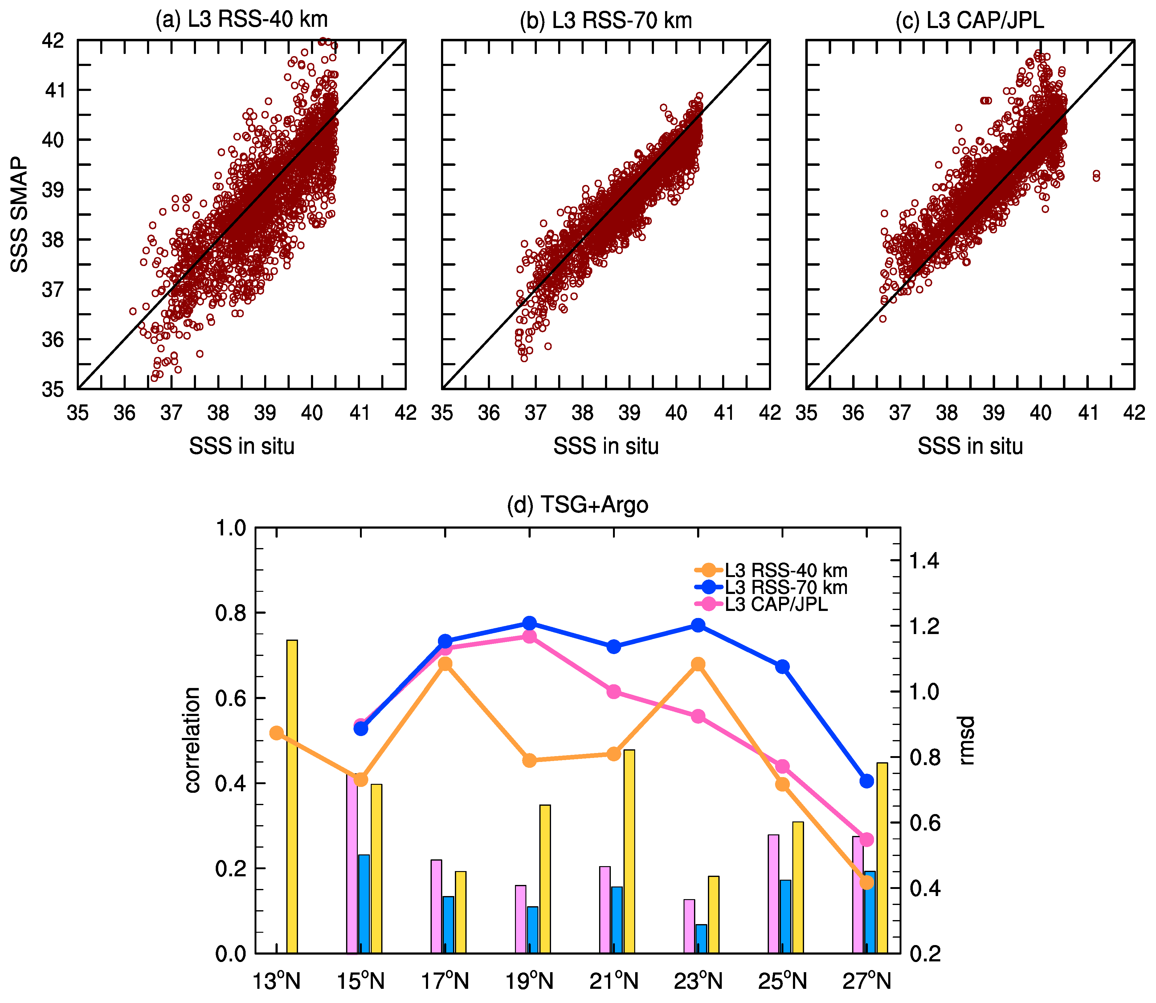
Tang et al. [3], using a previous version of the L3 CAP/JPL product, described correlations of 0.78 (TSG and Argo) and $rmsd$ of 0.52/0.56 (TSG/Argo) over 18 months in the Mediterranean Sea. The present study, the first to evaluate SMAP in the Red Sea, found correlations to be even higher (0.88/0.85, p-value < 0.001) and $rmsd$ even lower (0.59/0.46) for L3 CAP/JPL in the Red Sea. Note that the SMAP skill level in the Red Sea is indeed slightly better for the L3 RSS-70 km product (Table 10).

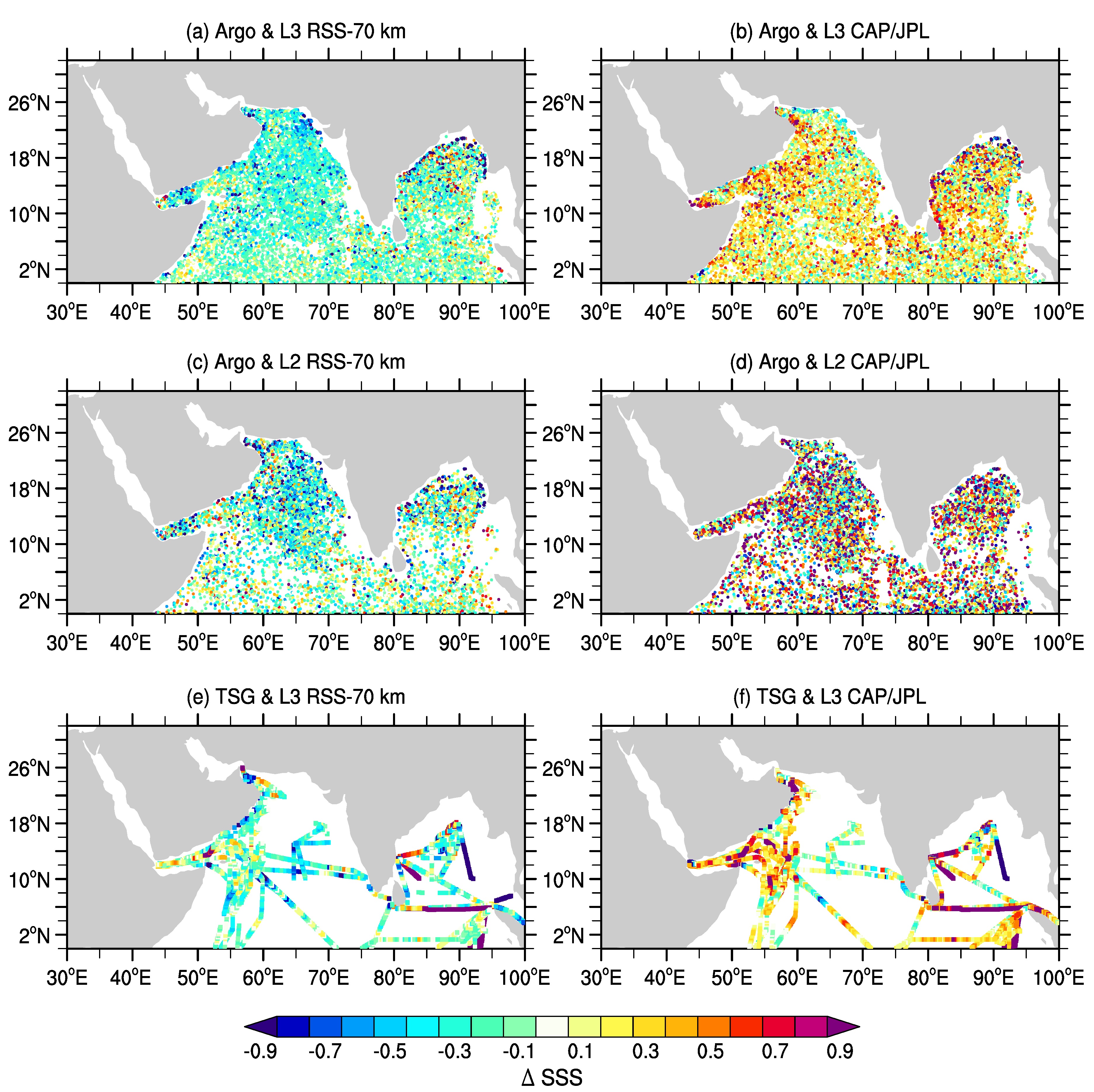
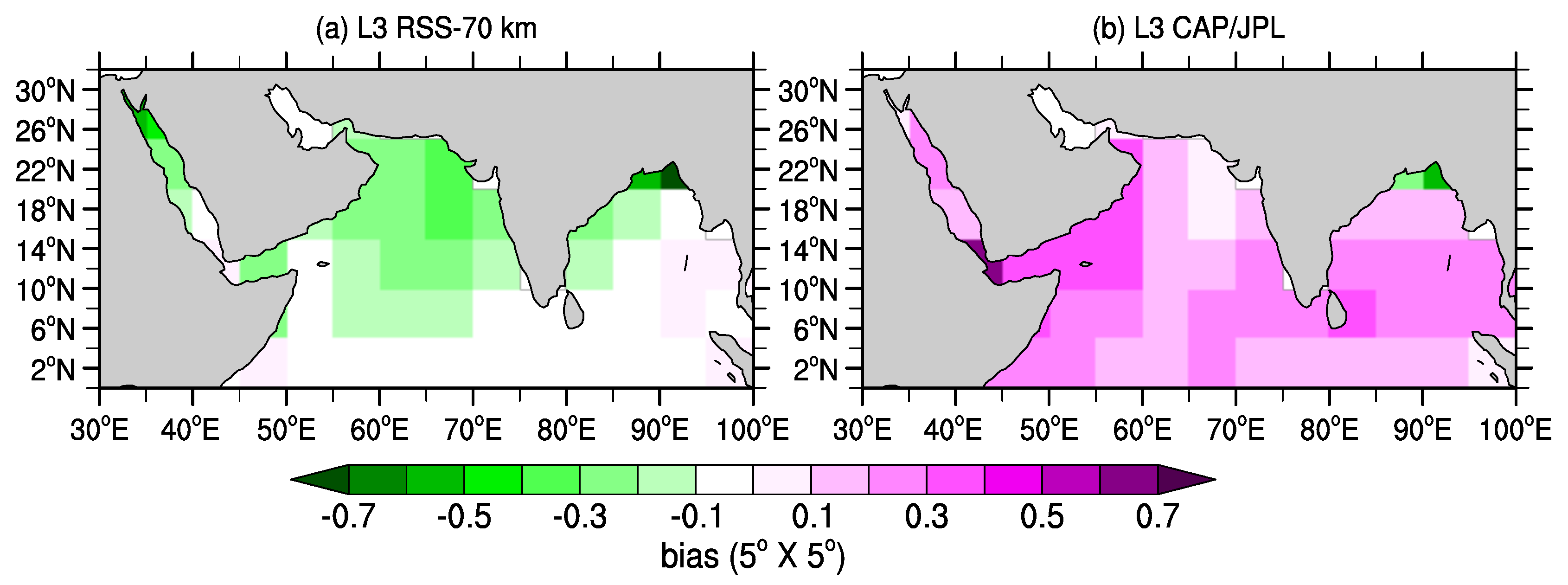
Different from the Mediterranean Sea, bias is consistent for a product series in the Red Sea, such as RSS products underestimate in situ SSS, and CAP/JPL ones overestimate it (independent if Argo or TSG observations are used for statistical comparison). In the Mediterranean Sea, bias is positive for the TSG and negative for Argo [3], but that was for a previous SMAP version than the ones used here. Moreover, there is no outstanding offset in Figure 14, such as in the Levantine area of the Mediterranean Sea (Figure 3a of Tang et al. [17]).

Within the Red Sea, SMAP performance is reduced in the extreme north and south (Figure 15), areas with less collocated data, and more prone to RFI and land contamination. Tang et al. [3] also described spatial differences in SMAP performance in the Mediterranean Sea due to these factors.

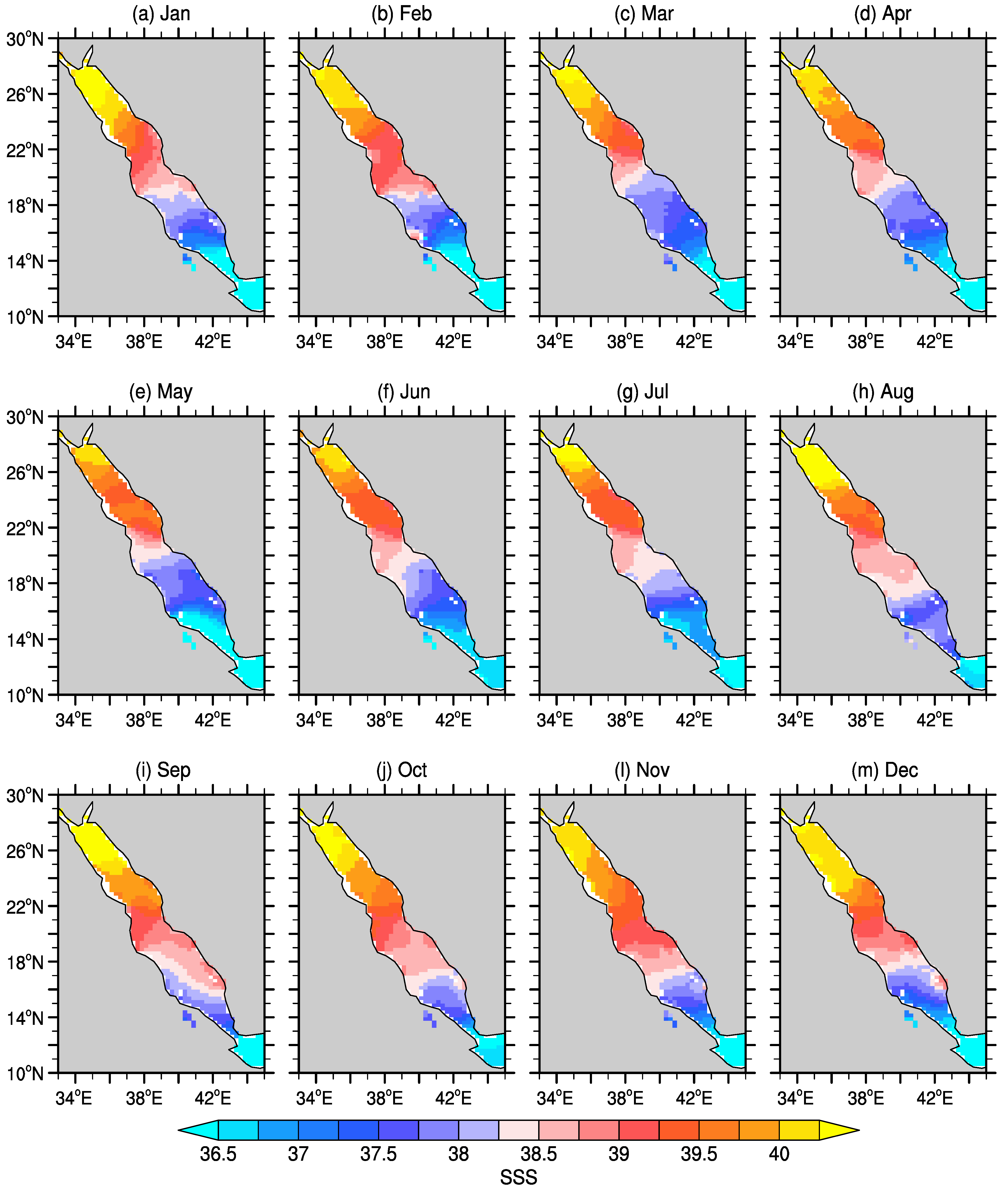
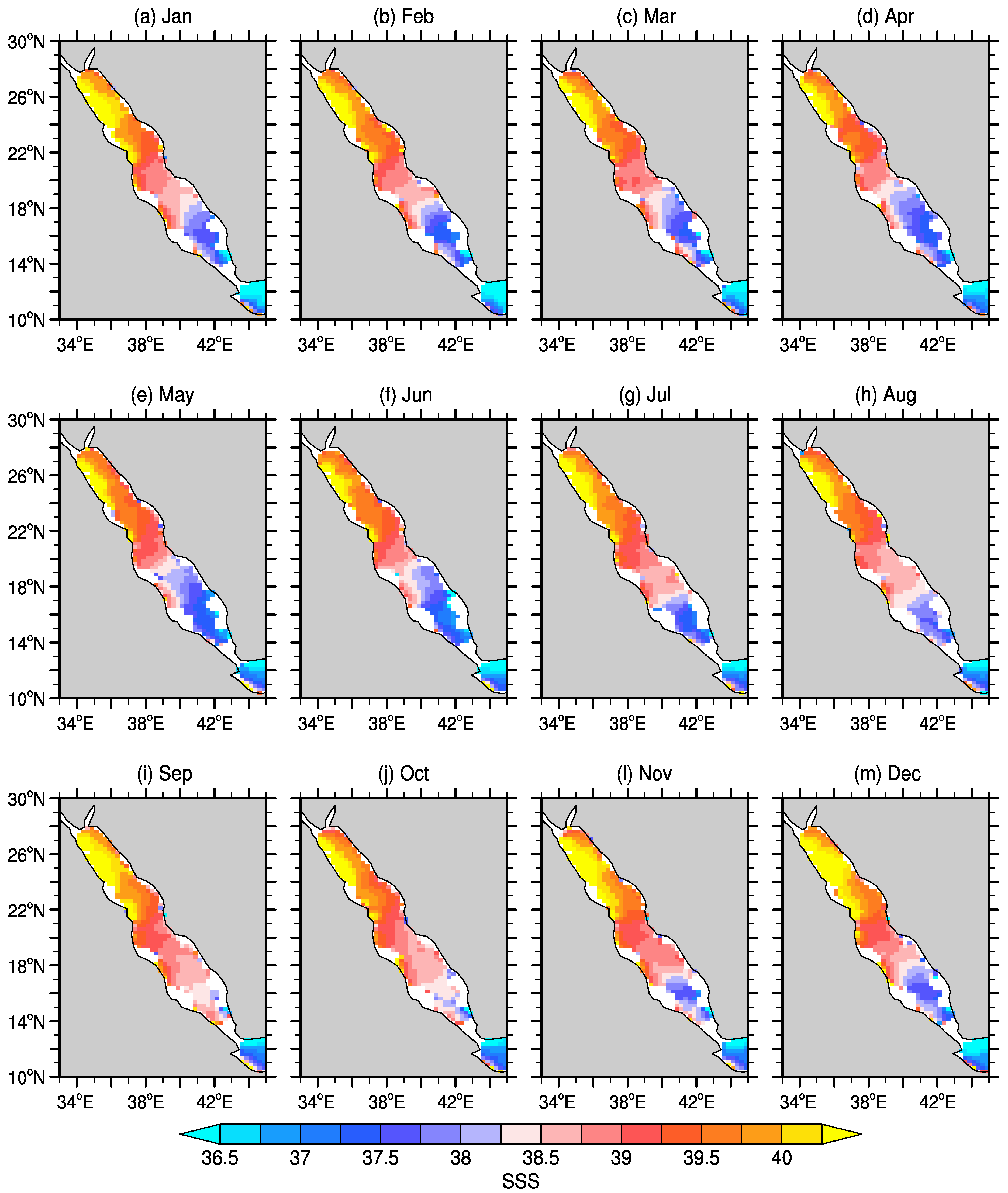
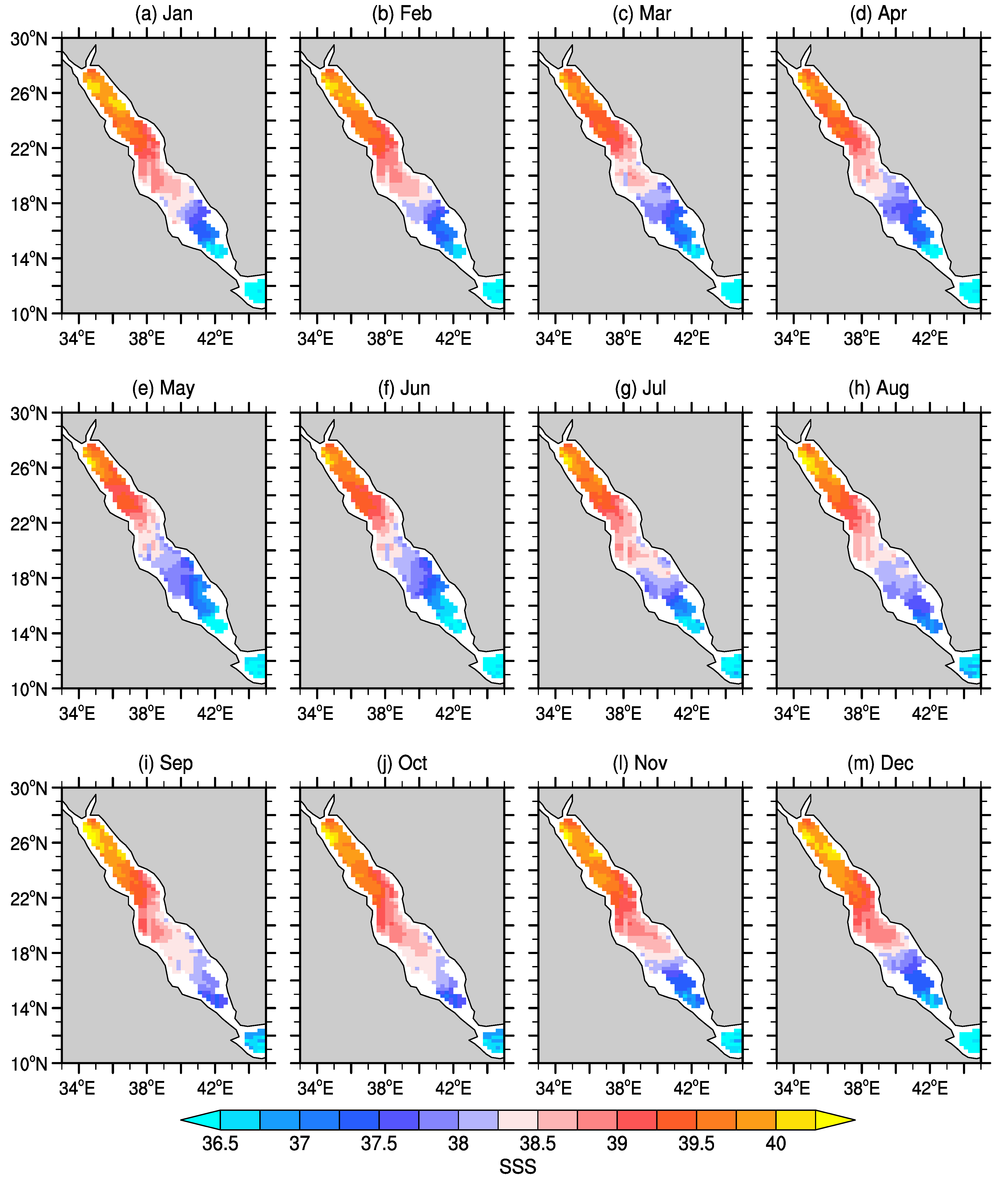
Seasonally, there is evidence that SMAP captures the intrusion of the fresher, colder, and nutrient-rich Gulf of Aden Surface Water (GASW) in winter [48,63]. Sofianos and Johns [48] described GASW as a relatively fresh surface inflow with salinity around 36–36.5. This description is similar to what SMAP shows (Figure 17 and Figure 18). SMAP SSS climatological maps also resemble the numerical simulations of Sofianos and Johns [54], with the eastern Red Sea slightly fresher than the western, especially north of 18°N (see also Figure S2). The SMAP SSS pattern would be consistent with the existence of a northward surface Eastern Boundary Current bringing warm and relatively fresh waters to the north, as described by Bower and Farrar [22]. However, the zonal difference in SMAP maps should be interpreted with caution given the moderate spatial resolution of the satellite, and possible RFI and land contamination. WOA18 does not show a clear zonal pattern in salinity, but its mapping scales are too wide. In conclusion, more work needs to be done to ensure that the SMAP zonal pattern is not an artifact due to RFI and land contamination.

The SMAP results in the Red Sea presented here are promising, particularly when they are contrasted with other marginal seas. For instance, Vazquez-Cuervo et al. [16] found correlations of 0.61–0.91 (except by one mooring in which correlation was around 0.3) and $rmsd$ of 0.4–0.78 in the much wider Gulf of Mexico for the L3 SMAP products they analyzed. These numbers are the same order as those described here for the narrow Red Sea.

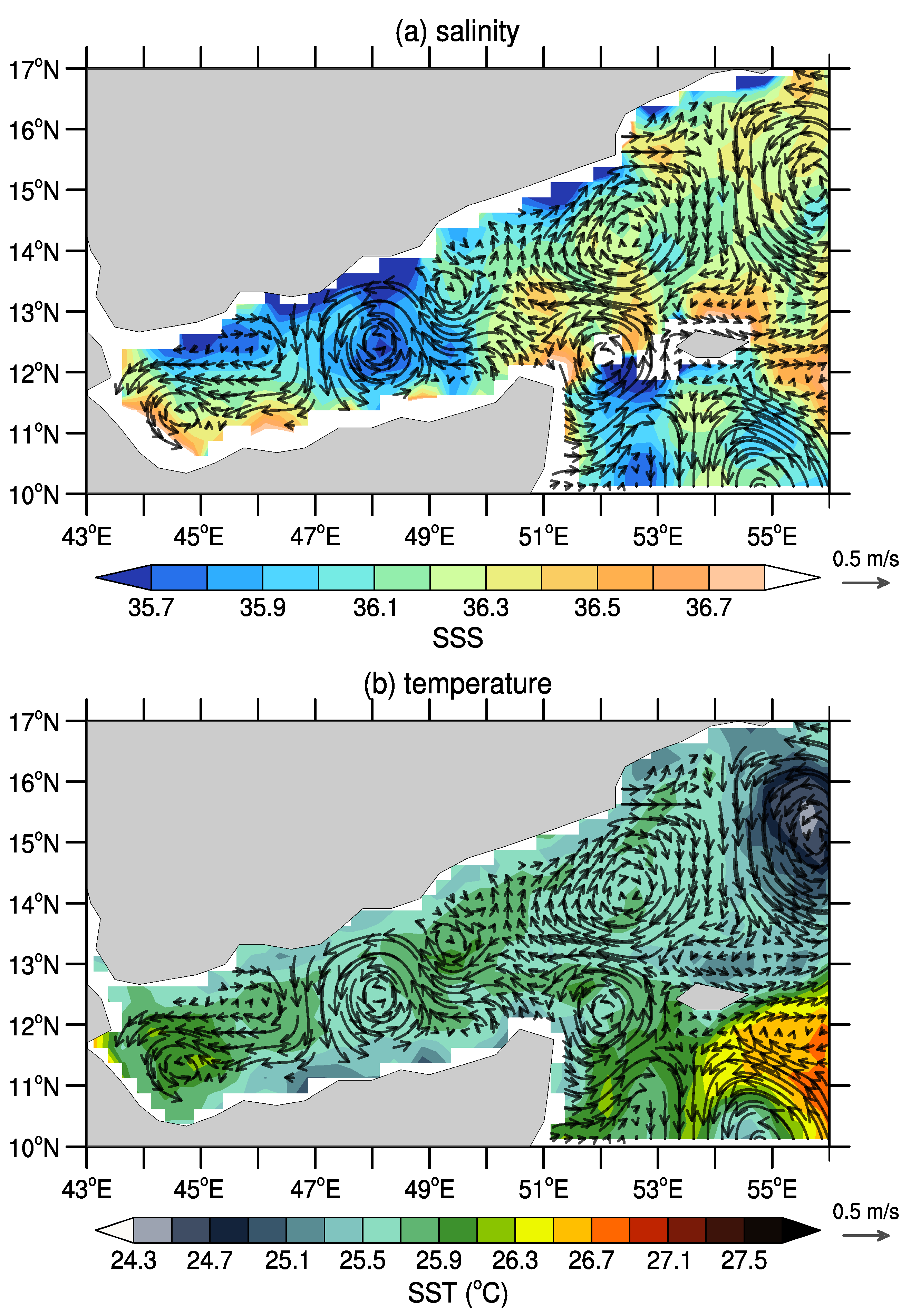
In the Gulf of Aden and Oman, SMAP performance is worse than that in the Red Sea, probably because RFI effects are more severe in the southward part of the Arabian Peninsula, although this study did not evaluate that. Despite this limitation, SMAP seems to capture signatures from mesoscale eddies in the Gulf of Aden. For instance, Figure 19 shows SSS and satellite-based sea-surface temperature (SST) fields for a random day in February 2019, overlaid with multisatellite altimetric geostrophic currents. Note that these datasets do not accurately represent the same period. A cyclonic (anticlockwise) eddy centered at 48°E and 12°N within the Gulf of Aden has a low salinity and temperature signature when compared with its surroundings. Mesoscale eddies are a crucial component of the Gulf of Aden dynamics, affecting Red Sea Overflow Water properties and the Gulf’s biogeochemistry [23,29,63,64]. Other agreements also exist in maps between mesoscale features, SSS and SST. However, new investigations are required before it can be ruled that SMAP is capturing mesoscale eddies in the Gulf of Aden, but these initial results are promising.

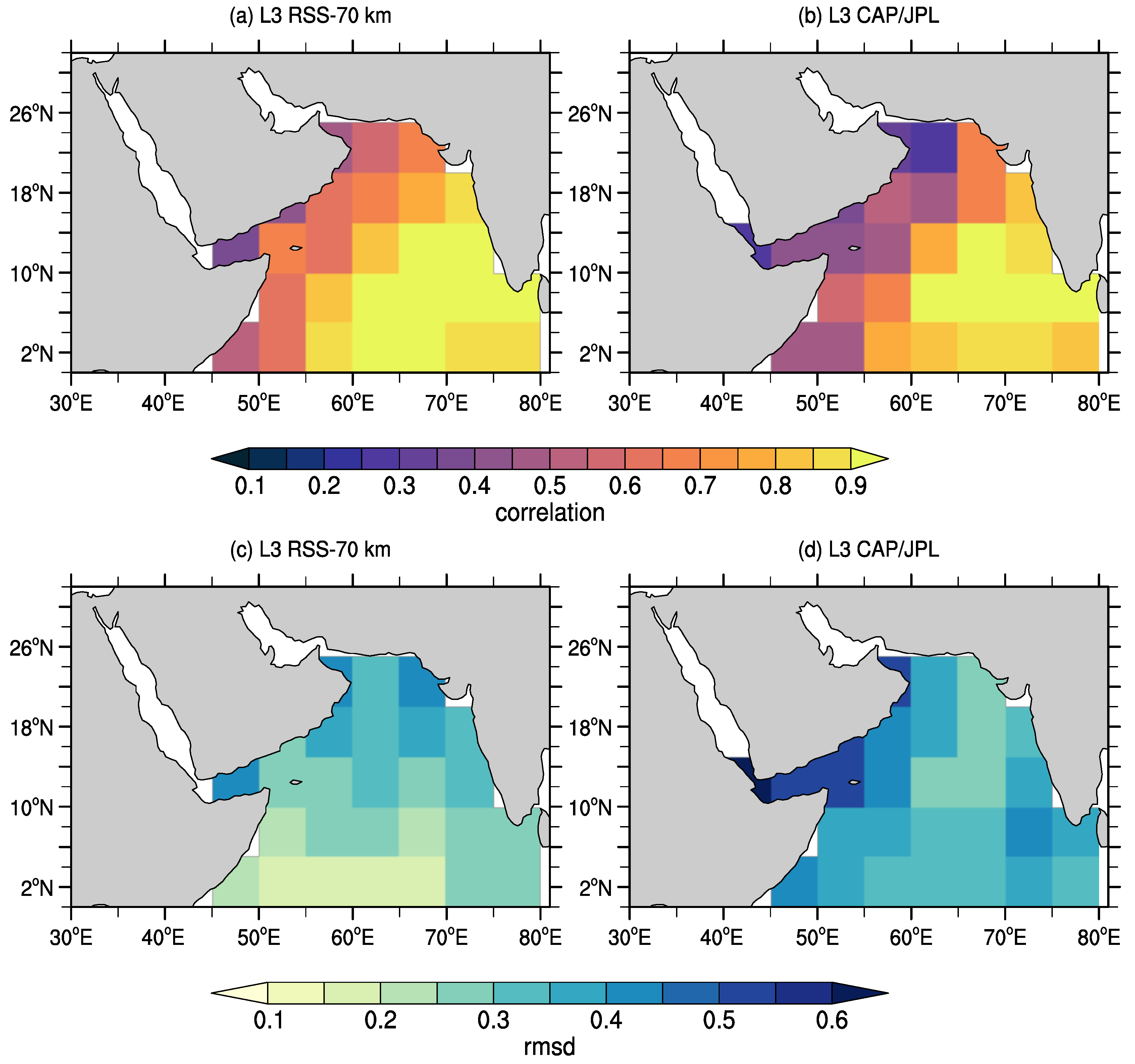
Within the Arabian Sea, there is a consistent improvement in SMAP statistical skills from the west, where the Gulfs of Aden and Oman are, to the east (Figure 8). Offshore the western boundary, all products show that SMAP captures SSS in the Arabian Sea with similar performance to the global evaluations [3,8], in which correlation in open water away from the coast is above 0.7 and $rmsd$ was less than 0.2

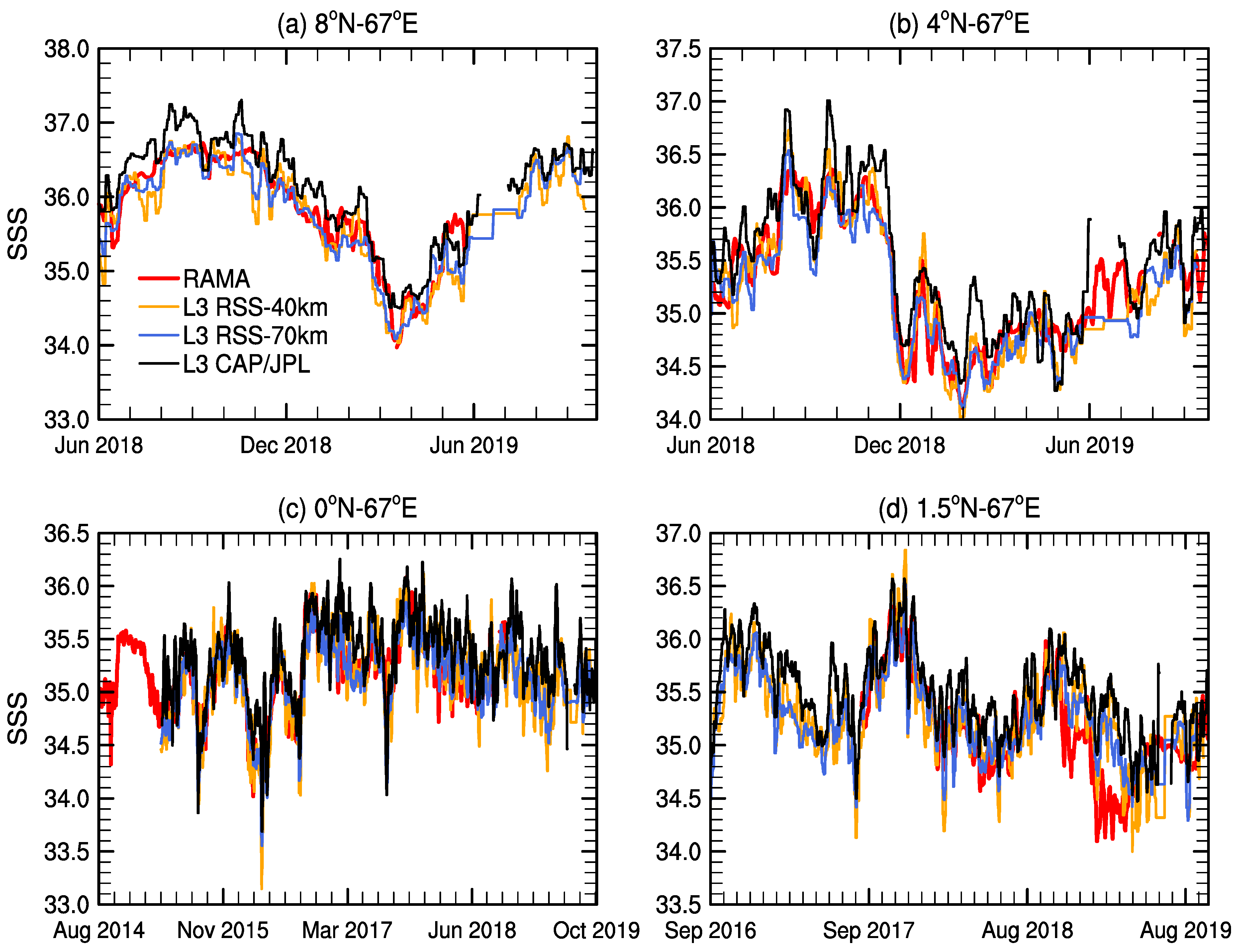
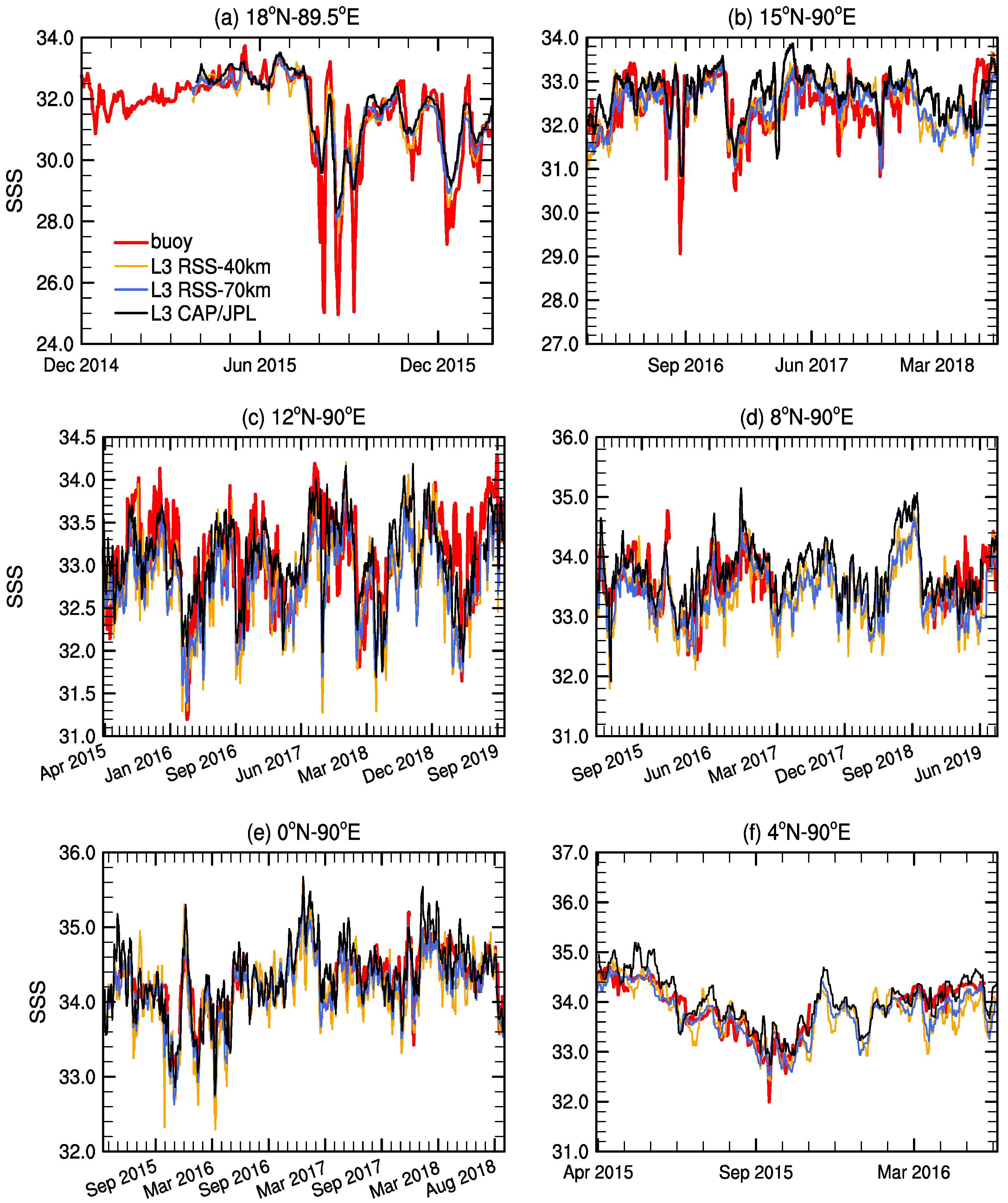
In the temporal domain, SMAP also reproduces the seasonal and subseasonal variability as measured by the RAMA array. Data from the RAMA array have also been previously used to validate SMAP [3], but at that time (April 2015–September 2016), there was no mooring outside the equatorial zone in the Arabian Sea. For the equatorial buoys in the western Indian Ocean, Tang et al. [3] found a high correlation (>0.7) and relatively low $rmsd$ (≈0.25). Here, statistics of the newest L3 CAP/JPL version over a much longer period (four years) are similar, with a correlation of 0.76 (0°N; 67°E) and 0.84 (1.5°N; 67°E), and $rmsd$ of 0.30 and 0.28, respectively. For the two moorings later deployed at 4°N and 8°N, correlations are even higher (Table 5).

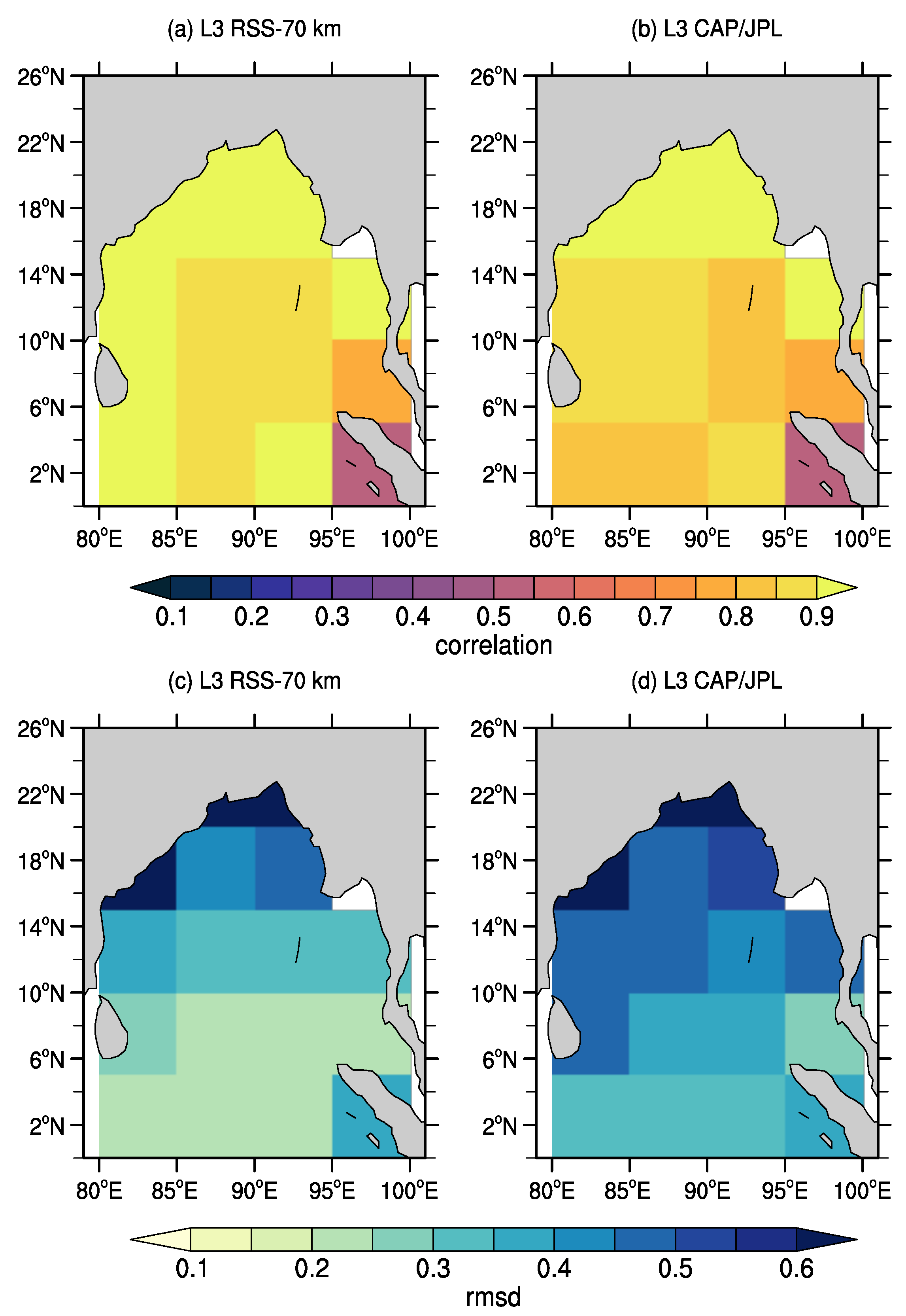
In the Bay of Bengal, statistics between the RAMA array and the CAP/JPL product follow a similar pattern, as shown in Tang et al. [3] (their Figure 8), with correlation decreasing and $rmsd$ increasing northward (Table 9). However, the spatial pattern from Argo does not show this northward worsening in SMAP retrieval (Figure 12). When compared with Argo, SMAP statistics are indeed better northward. As a point of fact, SMAP SSS is highly correlated (0.87–0.89) with observations at the WHOI mooring located in the northern part of the bay (18°N), with SMAP in-phase and capturing the timing of the intense drops in salinity measured at the buoy, although without the same intensity (Figure 13a).

Fournier et al. [18] compared a previous version of L3 CAP/JPL SMAP and all in situ SSS observations in the Bay of Bengal available at the World Ocean Database (which include Argo floats) between April 2015 and December 2016. In their 1.5 years collocated dataset, the correlation was 0.83, $rmsd$ 0.49, and there was a positive bias of 0.1. For the new version shown here and over four years, correlation is 0.95, $rmsd$ is more or less the same (0.44), but the positive bias is 0.2. However, the in situ data used as ground truth in both works are not quite the same.

5. Conclusions

The present study assessed SMAP SSS retrievals in the North Indian Ocean, particularly in the Arabian Sea and the Red Sea. The wide range of salinity of the North Indian Ocean, with SSS of less than 30 in the Bay of Bengal to more than 40 in the Red Sea, was attractive for evaluating the performance of the new SMAP versions in relation to in situ SSS. For this task, this work put together almost all in situ SSS observations publicly available over the SMAP era, which included Argo floats, TSG, ship-based CTD, and time series from moored buoys.

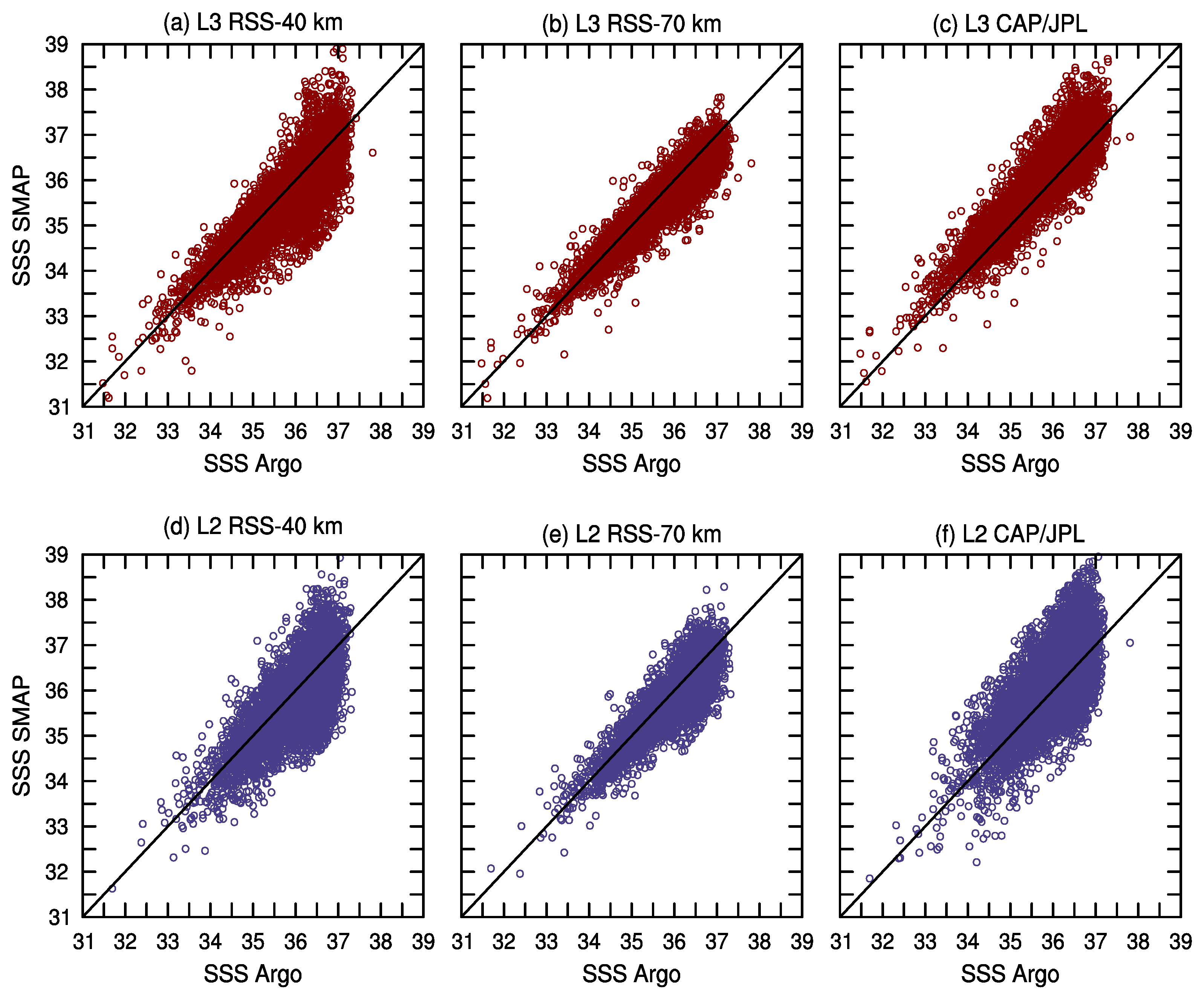
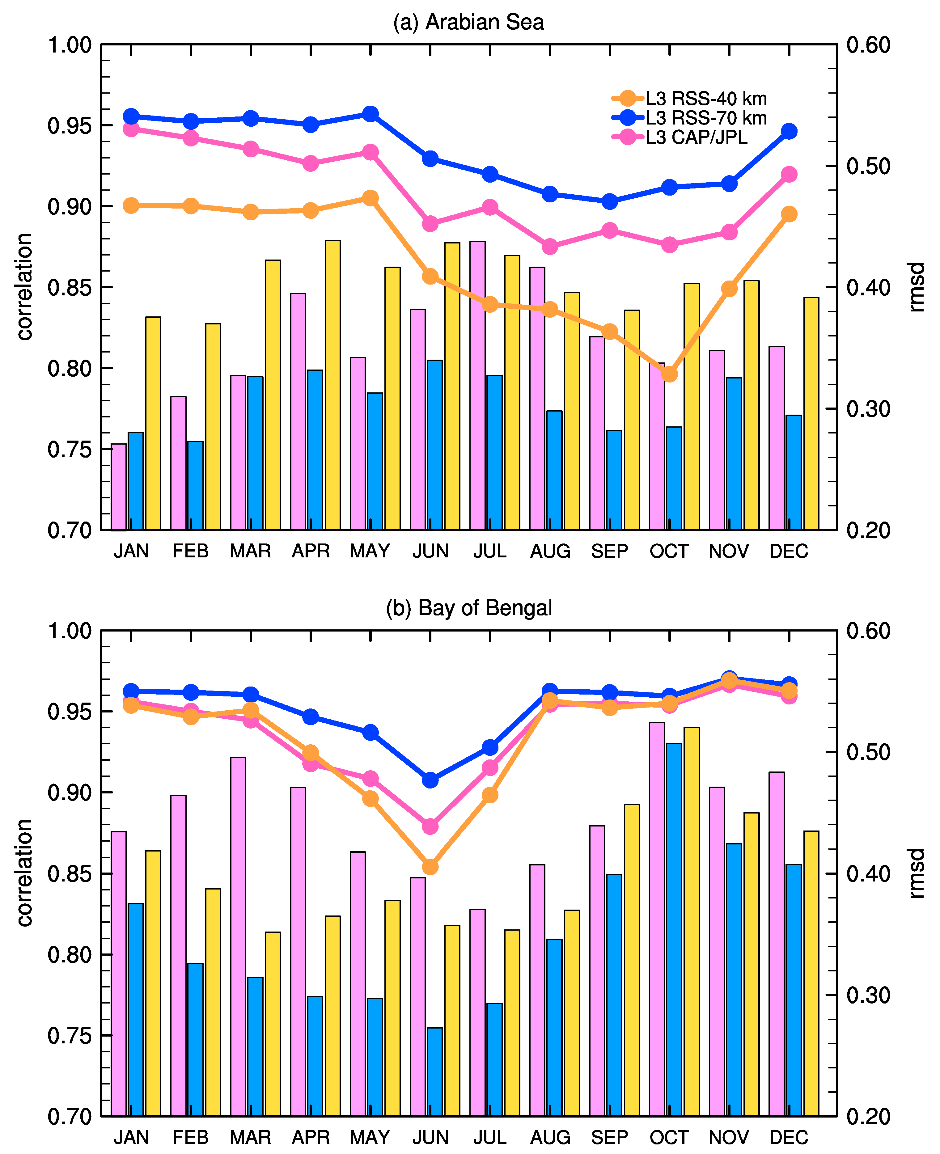
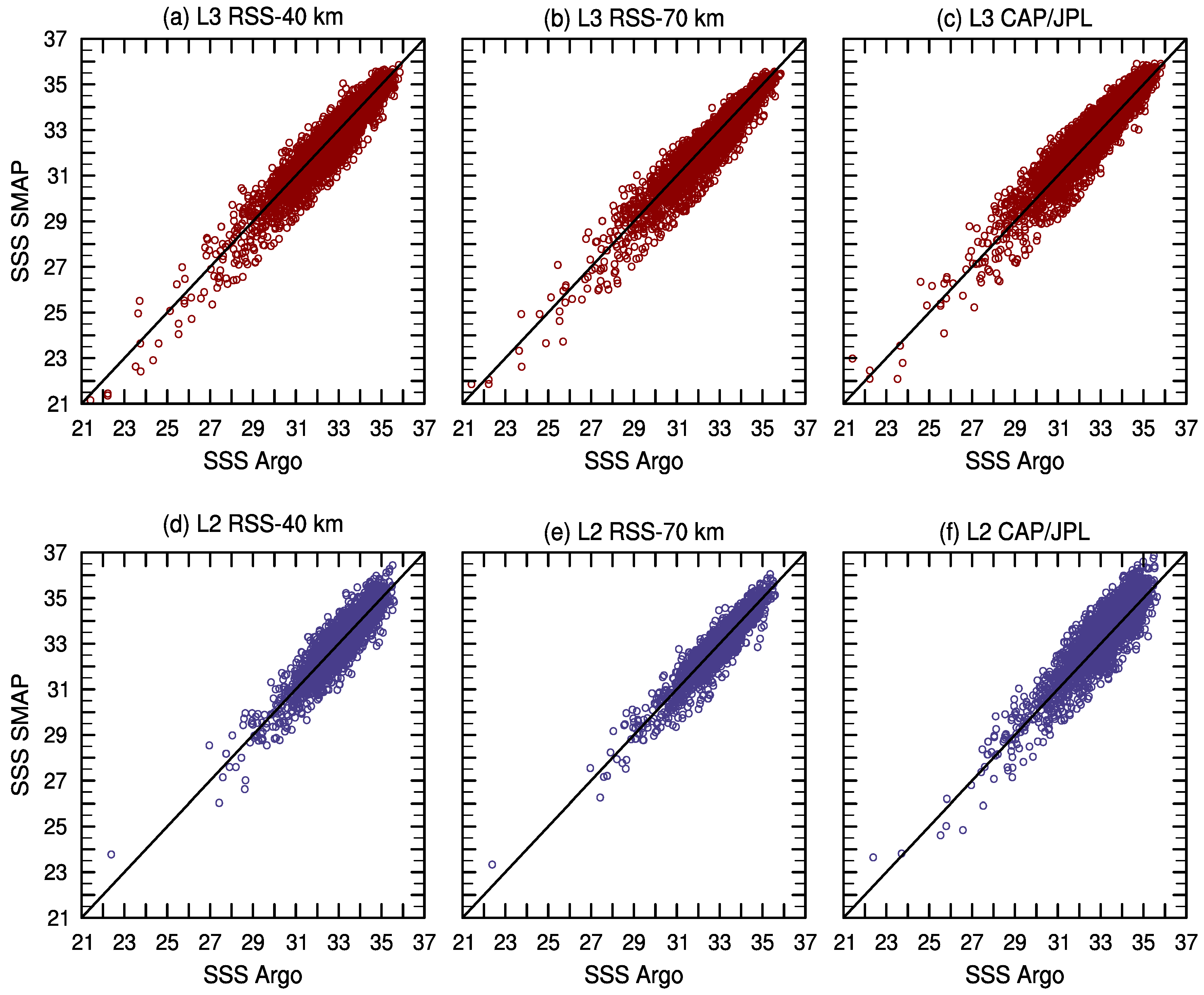
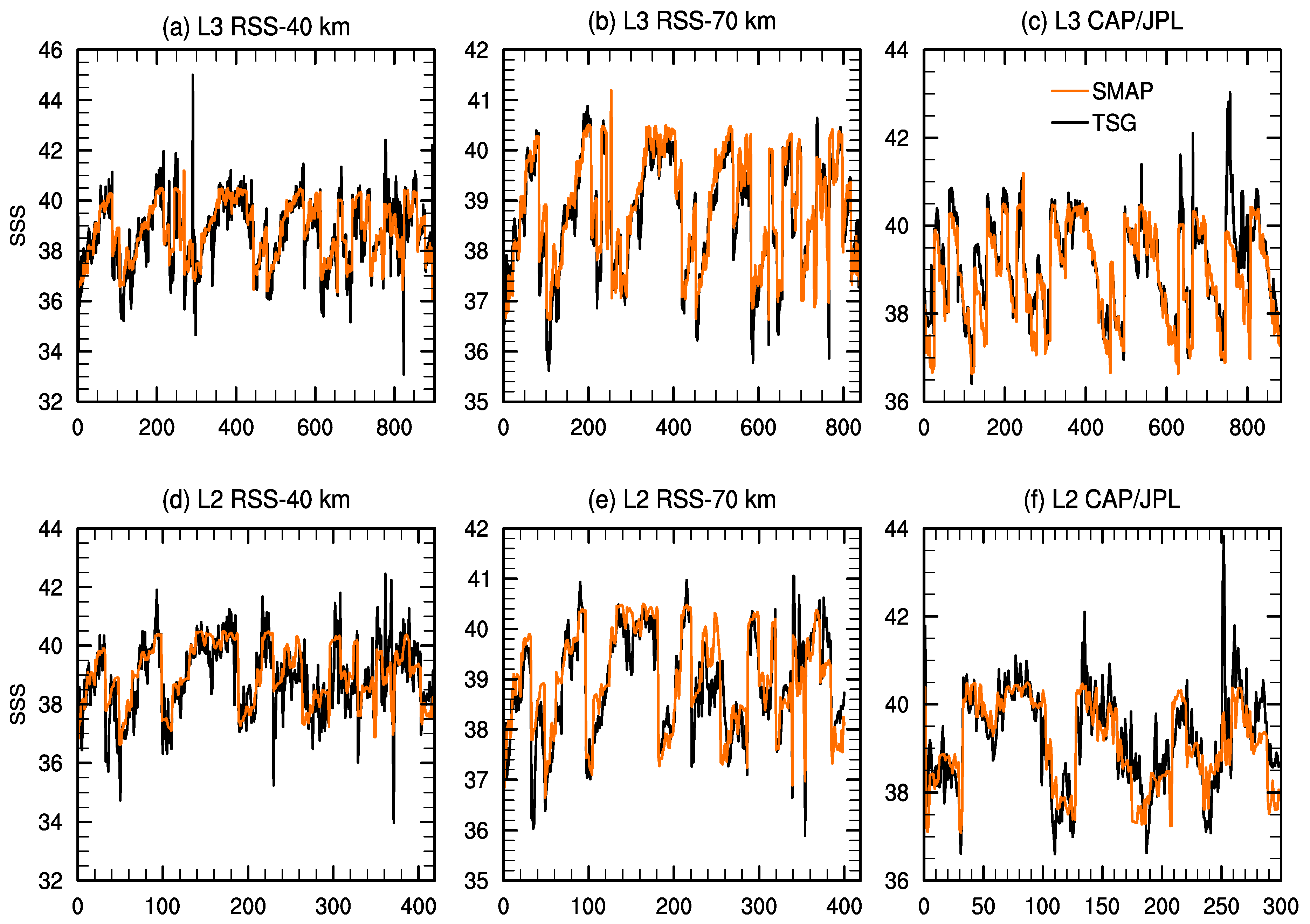
Overall, SMAP reproduces SSS relatively well with a high signal-to-noise ratio, in both the Arabian Sea and the Bay of Bengal, with correlation increasing, and $rmsd$ decreasing with spatial smoothing. Thus, CAP/JPL, with an effective spatial resolution of 60 km, tended to have a better performance than that of the RSS-40 km product, and slightly worse than that of the RSS-70 km. Similar improvement was observed when SMAP data is averaged over time, with the correlation being generally lower and $rmsd$ higher for L2 products when contrasted with the respective L3 datasets.

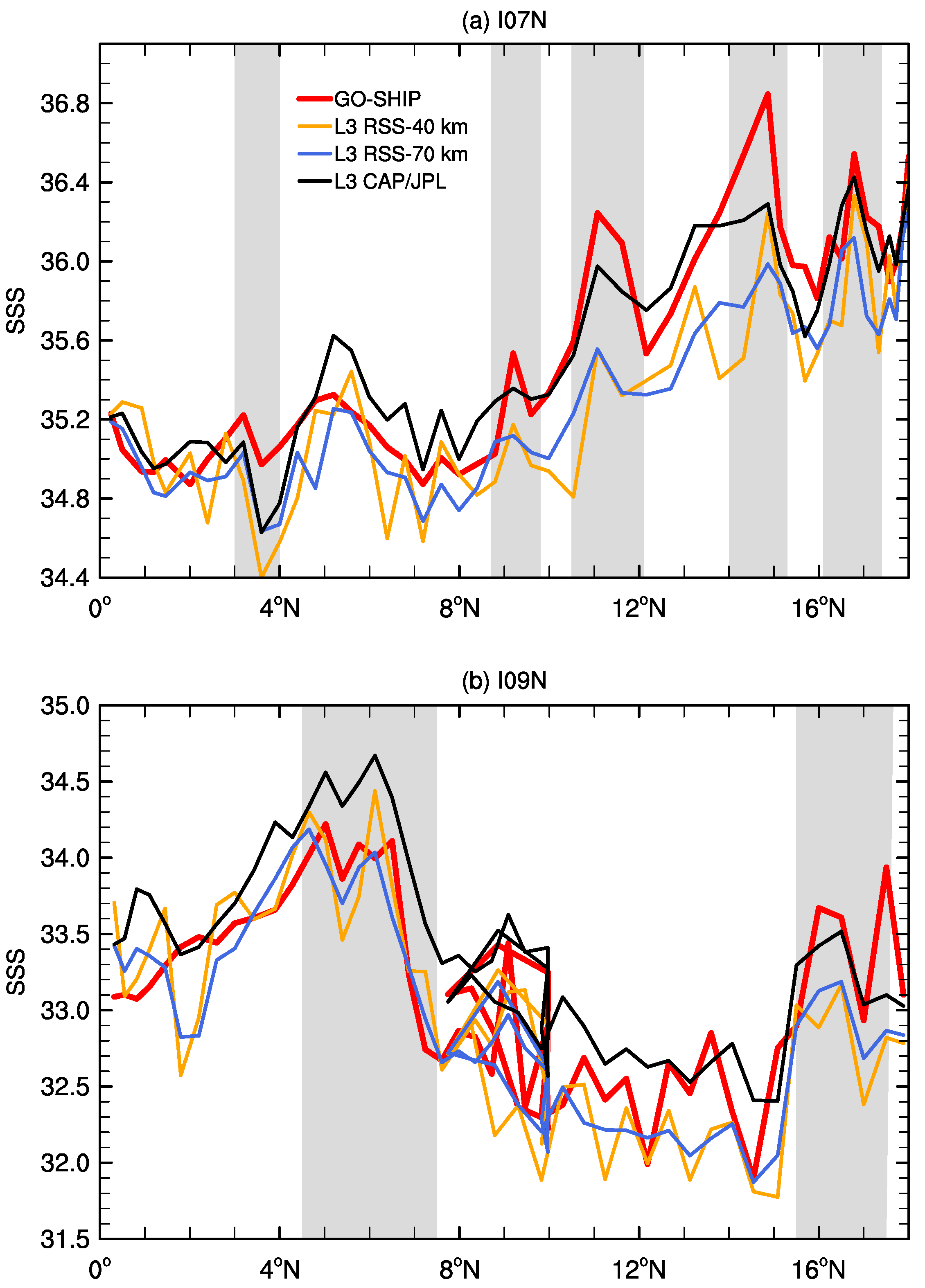
Furthermore, SMAP captures seasonal and subseasonal SSS variability, and also captures exceptionally well the sharp drops in salinity in the northern Bay of Bengal measured by the WHOI mooring, although with less intensity. The present work showed that there is seasonal sensitivity in SMAP’s skills, but the performance decrease is small and not equal in the western and eastern basin. In the Bay of Bengal, SMAP performance is lower in June while, in the Arabian Sea, it is around October. Interestingly, GO-SHIP hydrographic sections in the Arabian Sea and the Bay of Bengal give new evidence that SMAP can capture salinity features, which may be related to mesoscale eddies.

Agreement between the new SMAP products and Argo floats is better in the Bay of Bengal than that in the Arabian Sea, but this better agreement is not apparent when using TSG or RAMA data. Within the Arabian Sea, SMAP performance is much reduced on the western side for all products. This fact is particularly evident in the Gulfs of Aden and Oman. Skill reduction in these regions is possibly related to RFI contamination there, a subject to be further investigated. However, there is evidence that SMAP may be capturing SSS signatures due to mesoscale eddies in the Gulf of Aden, but this matter requires in-depth study.

On the other hand, SMAP retrievals in the narrow Red Sea are surprisingly good. SMAP statistics (with both TSG and Argo floats) are similar to the ones found in open-ocean water away from the coast. Results there encourage the development of a specially designed SMAP product in this marginal sea where the scarcity of SSS observations is historical, and not much is known about SSS variability [22,48]. One could imagine designing a product by using more advanced filtering techniques to remove spatial noise in L2 data, such as the ones based on singular spectrum analysis used by Menezes et al. [61], and an optimal interpolation scheme to map SMAP L2-filtered data into a regular grid instead of simple average binning.

A still-present limitation in both RSS and CAP/JPL products is the bias in the entire North Indian Ocean. However, because the bias is consistent and spatially homogeneous, as shown here, it should not affect studies about temporal SSS variability in the North Indian Ocean, which is the next step in this project. Issues still to be thoroughly investigated are the possible effects of RFI contamination, particularly in the Gulf of Oman, and precipitation in the Bay of Bengal during the summer monsoon. However, in the latter case, the in situ data currently available are not the most adequate since Argo floats do not capture possible near-surface stratification (0–5 m) that may occur in heavy rainfall.

References

1. Dinnat, E.; Le Vine, D.; Boutin, J.; Meissner, T.; Lagerloef, G. Remote Sensing of Sea Surface Salinity: Comparison of Satellite and In Situ Observations and Impact of Retrieval Parameters. Remote Sens. 2019, 11, 750. [Google Scholar] [CrossRef] [Green Version]
2. Meissner, T.; Wentz, F.J.; Le Vine, D.M. The Salinity Retrieval Algorithms for the NASA Aquarius Version 5 and SMAP Version 3 Releases. Remote Sens. 2018, 10, 1121. [Google Scholar] [CrossRef] [Green Version]
3. Tang, W.; Fore, A.; Yueh, S.; Lee, T.; Hayashi, A.; Sanchez-Franks, A.; Martinez, J.; King, B.; Baranowski, D. Validating SMAP SSS with in situ measurements. Remote Sens. Environ. 2017, 200, 326–340. [Google Scholar] [CrossRef] [Green Version]
4. Vinogradova, N.; Lee, T.; Boutin, J.; Fournier, S.; Sabia, R.; Stammer, D.; Bayler, E.; Reul, N.; Gordon, A.; Melnichenko, O.; et al. Satellite Salinity Observing System: Recent Discoveries and the Way Forward. Front. Mar. Sci. 2019, 6, 243. [Google Scholar] [CrossRef]
5. Le Vine, D.M.; Johnson, J.T.; Piepmeier, J. RFI and Remote Sensing of the Earth From Space. In Proceedings of the Radio Frequency Interference (RFI) 2016 Conference, Socorro, NM, USA, 17–20 October 2016. [Google Scholar] [CrossRef] [Green Version]
6. Meissner, T.; Wentz, F.J.; Manaster, A.; Lindsley, R. Remote Sensing Systems SMAP Ocean Surface Salinities [Level 2C, Level 3 Running 8-day, Level 3 Monthly], Version 4.0 Validated Release; Remote Sensing Systems: Santa Rosa, CA, USA, 2019. [Google Scholar] [CrossRef]
7. Fore, A.; Yueh, S.; Tang, W.; Hayashi, A. SMAP Salinity and Wind Speed Data User’s Guide–Version 4.2; Technical Report; Jet Propulsion Laboratory, California Institute of Technology: Pasadena, CA, USA, 2019.
8. Bao, S.; Wang, H.; Zhang, R.; Yan, H.; Chen, J. Comparison of satellite-derived sea surface salinity products from SMOS, Aquarius, and SMAP. J. Geophys. Res. Ocean. 2019, 124, 1932–1944. [Google Scholar] [CrossRef]
9. Tang, W.; Yueh, S.; Yang, D.; Fore, A.; Hayashi, A.; Lee, T.; Fournier, S.; Holt, B. The Potential and Challenges of Using Soil Moisture Active Passive (SMAP) Sea Surface Salinity to Monitor Arctic Ocean Freshwater Changes. Remote Sens. 2018, 10, 869. [Google Scholar] [CrossRef] [Green Version]
10. da Silva, C.E.; Castelao, R.M. Mississippi River plume variability in the Gulf of Mexico from SMAP and MODIS-Aqua observations. J. Geophys. Res. Ocean. 2018, 123, 6620–6638. [Google Scholar] [CrossRef]
11. Fournier, S.; Reager, J.T.; Lee, T.; Vazquez-Cuervo, J.; David, C.H.; Gierach, M.M. SMAP observes flooding from land to sea: The Texas event of 2015. Geophys. Res. Lett. 2016, 43, 10338–10346. [Google Scholar] [CrossRef]
12. Vazquez-Cuervo, J.; Fournier, S.; Dzwonkowski, B.; Reager, J. Intercomparison of In-Situ and Remote Sensing Salinity Products in the Gulf of Mexico, a River-Influenced System. Remote Sens. 2018, 10, 1590. [Google Scholar] [CrossRef] [Green Version]
13. Grodsky, S.; Vandemark, D.; Feng, H. Assessing Coastal SMAP Surface Salinity Accuracy and Its Application to Monitoring Gulf of Maine Circulation Dynamic. Remote Sens. 2018, 10, 1232. [Google Scholar] [CrossRef] [Green Version]
14. Grodsky, S.A.; Vandemark, D.; Feng, H.; Levin, J. Satellite detection of an unusual intrusion of salty slope water into a marginal sea: Using SMAP to monitor Gulf of Maine inflows. Remote Sens. Environ. 2018, 217, 550–561. [Google Scholar] [CrossRef]
15. Vazquez-Cuervo, J.; Gomez-Valdes, J. SMAP and CalCOFI Observe Freshening during the 2014-2016 Northeast Pacific Warm Anomaly. Remote Sens. 2018, 10, 1716. [Google Scholar] [CrossRef] [Green Version]
16. Vazquez-Cuervo, J.; Gomez-Valdes, J.; Bouali, M.; Miranda, L.; Van der Stocken, T.; Tang, W.; Gentemann, C. Using Saildrones to Validate Satellite-Derived Sea Surface Salinity and Sea Surface Temperature along the California/Baja Coast. Remote Sens. 2019, 11, 1964. [Google Scholar] [CrossRef] [Green Version]
17. Grodsky, S.A.; Reul, N.; Bentamy, A.; Vandemark, D.; Guimbard, S. Eastern Mediterranean salinification observed in satellite salinity from SMAP mission. J. Mar. Syst. 2019, 198, 103190. [Google Scholar] [CrossRef]
18. Fournier, S.; Vialard, J.; Lengaigne, M.; Lee, T.; Gierach, M.M.; Chaitanya, A.V.S. Modulation of the Ganges-Brahmaputra river plume by the Indian Ocean dipole and eddies inferred from satellite observations. J. Geophys. Res. Ocean. 2017, 122, 9591–9604. [Google Scholar] [CrossRef] [Green Version]
19. Lee, T.; Fournier, S.; Gordon, A.; Sprintall, J. Maritime Continent water cycle regulates low-latitude chokepoint of global ocean circulation. Nat. Commun. 2019, 2103. [Google Scholar] [CrossRef] [Green Version]
20. Ferster, B.S.; Subrahmanyam, B. A Comparison of Satellite-Derived Sea Surface Salinity and Salt Fluxes in the Southern Ocean. Remote Sens. Earth Syst. Sci. 2018, 1, 1–13. [Google Scholar] [CrossRef]
21. Garcia-Eidell, C.; Comiso, J.C.; Dinnat, E.; Brucker, L. Sea surface salinity distribution in the Southern Ocean as observed from space. J. Geophys. Res. Ocean. 2019, 124, 3186–3205. [Google Scholar] [CrossRef]
22. Bower, A.S.; Farrar, J.T. Air-Sea Interaction and Horizontal Circulation in the Red Sea. In The Red Sea; Rasul, N.M.A., Stewart, I.C.F., Eds.; Springer: Berlin/Heidelberg, Germany, 2015; pp. 329–342. [Google Scholar] [CrossRef]
23. Bower, A.S.; Furey, H.H. Mesoscale eddies in the Gulf of Aden and their impact on the spreading of Red Sea Outflow Water. Prog. Oceanogr. 2012, 96, 14–39. [Google Scholar] [CrossRef] [Green Version]
24. Beal, L.M.; Ffield, A.; Gordon, A.L. Spreading of Red Sea overflow waters in the Indian Ocean. J. Geophys. Res. 2000, 105, 8549–8564. [Google Scholar] [CrossRef]
25. Beal, L.M.; Hormann, V.; Lumpkin, R.; Foltz, G.R. The Response of the Surface Circulation of the Arabian Sea to Monsoonal Forcing. J. Phys. Oceanogr. 2013, 43, 2008–2022. [Google Scholar] [CrossRef] [Green Version]
26. Brandt, P.; Stramma, L.; Schott, F.; Fischer, J.; Dengler, M.; Quadfasel, D. Annual Rossby waves in the Arabian Sea from TOPEX/POSEIDON altimeter and in situ data. Deep-Sea Res. II 2002, 49, 1197–1210. [Google Scholar] [CrossRef]
27. Fischer, A.S.; Weller, R.A.; Rudnick, D.L.; Eriksen, C.C.; Lee, C.M.; Brink, K.H.; Fox, C.A.; Leben, R.R. Mesoscale eddies, coastal upwelling, and the upper-ocean heat budget in the Arabian Sea. Deep-Sea Res. II 2002, 49, 2231–2264. [Google Scholar] [CrossRef]
28. Fratantoni, D.M.; Bower, A.S.; Johns, W.E.; Peters, H. Somali Current rings in the eastern Gulf of Aden. J. Geophys. Res. 2006, 111, C09039. [Google Scholar] [CrossRef] [Green Version]
29. Al Saafani, M.A.; Shenoi, S.S.C.; Shankar, D.; Aparna, M.; Kurian, J.; Durand, F.; Vinayachandran, P.N. Westward movement of eddies into the Gulf of Aden from the Arabian Sea. J. Geophys. Res. 2007, 112, C11004. [Google Scholar] [CrossRef]
30. Trott, C.B.; Subrahmanyam, B.; Chaigneau, A.; Roman-Stork, H.L. Eddy-induced temperature and salinity variability in the Arabian Sea. Geophys. Res. Lett. 2019, 46, 2734–2742. [Google Scholar] [CrossRef]
31. Subrahmanyam, B.; Trott, C.B.; Murty, V.S.N. Detection of Intraseasonal Oscillations in SMAP salinity in the Bay of Bengal. Geophys. Res. Lett. 2018, 45, 7057–7065. [Google Scholar] [CrossRef]
32. Sloyan, B.M.; Wanninkhof, R.; Kramp, M.; Johnson, G.C.; Talley, L.D.; Tanhua, T.; McDonagh, E.; Cusack, C.; O’Rourke, E.; McGovern, E.; et al. The Global Ocean Ship-Based Hydrographic Investigations Program (GO-SHIP): A Platform for Integrated Multidisciplinary Ocean Science. Front. Mar. Sci. 2019, 6, 445. [Google Scholar] [CrossRef] [Green Version]
33. Boutin, J.; Chao, Y.; Asher, W.E.; Delcroix, T.; Drucker, R.; Drushka, K.; Kolodziejczyk, N.; Lee, T.; Reul, N.; Reverdin, G.; et al. Satellite and In Situ Salinity: Understanding Near-Surface Stratification and Subfootprint Variability. Bull. Am. Meteorol. Soc. 2016, 97, 1391–1407. [Google Scholar] [CrossRef] [Green Version]
34. D’Addezio, J.M.; Bingham, F.M.; Jacobs, G.A. Sea surface salinity subfootprint variability estimates from regional high-resolution model simulations. Remote Sens. Environ. 2019, 233, 111365. [Google Scholar] [CrossRef]
35. Bingham, F. Subfootprint Variability of Sea Surface Salinity Observed during the SPURS-1 and SPURS-2 Field Campaigns. Remote Sens. 2019, 11, 2689. [Google Scholar] [CrossRef] [Green Version]
36. Roemmich, D.; Gilson, J. The 2004-2008 mean and annual cycle of temperature, salinity, and steric height in the global ocean from the Argo Program. Progr. Oceanogr. 2009, 82, 81–100. [Google Scholar] [CrossRef]
37. D’Addezio, J.M.; Subrahmanyam, B.; Nyadjro, E.S.; Murty, V.S.N. Seasonal Variability of Salinity and Salt Transport in the Northern Indian Ocean. J. Phys. Oceanogr. 2015, 45, 1947–1966. [Google Scholar] [CrossRef]
38. Akhil, V.P.; Durand, F.; Lengaigne, M.; Vialard, J.; Keerthi, M.G.; Gopalakrishna, V.V.; Deltel, C.; Papa, F.; de Boyer Montegut, C. A modeling study of the processes of surface salinity seasonal cycle in the Bay of Bengal. J. Geophys. Res. Ocean. 2014, 119, 3926–3947. [Google Scholar] [CrossRef] [Green Version]
39. Han, W.; McCreary, J. Modeling salinity distributions in the Indian Ocean. J. Geophys. Res. 2001, 206, 859–877. [Google Scholar] [CrossRef]
40. Llovel, W.; Lee, T. Importance and origin of halosteric contribution to sea level change in the southeast Indian Ocean during 2005–2013. Geophys. Res. Lett 2015, 42, 1148–1157. [Google Scholar] [CrossRef]
41. Nyadjro, E.S.; Subrahmanyam, B.; Shriver, J.F. Seasonal variability of salt transport during the Indian Ocean monsoons. J. Geophys. Res. 2011, 116, C08036. [Google Scholar] [CrossRef] [Green Version]
42. Nyadjro, E.S.; Subrahmanyam, B.; Murty, V.S.N.; Shriver, J.F. The role of salinity on the dynamics of the Arabian Sea mini warm pool. J. Geophys. Res. 2012, 117, C09002. [Google Scholar] [CrossRef]
43. Nyadjro, E.S.; Subrahmanyam, B.; Giesec, B.S. Variability of salt flux in the Indian Ocean during 1960–2008. Remote Sens. Environ. 2013, 134, 175–193. [Google Scholar] [CrossRef]
44. Swift, S.A.; Bower, A.S. Formation and circulation of dense water in the Persian/Arabian Gulf. J. Geophys. Res. 2003, 108, 3004. [Google Scholar] [CrossRef]
45. Murray, S.P.; Johns, W. Direct observations of seasonal exchange through the Bab el Mandab Strait. Geophys. Res. Lett 1997, 24, 2557–2560. [Google Scholar] [CrossRef]
46. Sofianos, S.S.; Johns, W.E.; Murray, S.P. Heat and freshwater budgets in the Red Sea from direct observations at Bab el Mandeb. Deep-Sea Res. II 2002, 49, 1323–1340. [Google Scholar] [CrossRef]
47. Sofianos, S.S.; Johns, W.E. Observations of the summer Red Sea circulation. J. Geophys. Res. 2007, 112, C06025. [Google Scholar] [CrossRef]
48. Sofianos, S.S.; Johns, W.E. Water Mass Formation, Overturning Circulation, and the Exchange of the Red Sea with the Adjacent Basins. In The Red Sea; Rasul, N.M.A., Stewart, I.C.F., Eds.; Springer: Berlin/Heidelberg, Germany, 2015; pp. 343–354. [Google Scholar] [CrossRef]
49. Yao, F.; Hoteit, I.; Pratt, L.J.; Bower, A.S.; Zhai, P.; Kohl, A.; Gopalakrishnan, G. Seasonal overturning circulation in the Red Sea: 1. Model validation and summer circulation. J. Geophys. Res. Ocean. 2014, 119, 2238–2262. [Google Scholar] [CrossRef] [Green Version]
50. Yao, F.; Hoteit, I.; Pratt, L.J.; Bower, A.S.; Kohl, A.; Gopalakrishnan, G.; Rivas, D. Seasonal overturning circulation in the Red Sea: 2. Winter circulation. J. Geophys. Res. Ocean. 2014, 119, 2263–2289. [Google Scholar] [CrossRef] [Green Version]
51. Menezes, V.V.; Farrar, J.; Bower, A. Evaporative implications of dry-air outbreaks over the northern Red Sea. J. Geophys. Res. Atmos. 2019, 124, 4829–4861. [Google Scholar] [CrossRef] [Green Version]
52. Tragou, E.; Garrett, C.; Outerbridge, R.; Gilman, C. The Heat and Freshwater Budgets of the Red Sea. J. Phys. Oceanogr. 1999, 29, 2504–2522. [Google Scholar] [CrossRef]
53. Zolina, O.; Dufour, A.; Gulev, S.; Stenchikov, G. Regional Hydrological Cycle over the Red Sea in ERA-Interim. J. Hydrometeorol. 2017, 18, 65–83. [Google Scholar] [CrossRef] [Green Version]
54. Sofianos, S.S.; Johns, W.E. An Oceanic General Circulation Model (OGCM) investigation of the Red Sea circulation: 2. Three-dimensional circulation in the Red Sea. J. Geophys. Res. 2003, 108, 3066. [Google Scholar] [CrossRef] [Green Version]
55. IOC; SCOR; IAPSO. The International Thermodynamic Equation of Seawater–2010: Calculation and Use of Thermodynamic Properties; Intergovernmental Oceanographic Commission, Manuals and Guides 56; UNESCO: London, UK, 2010; 196p. [Google Scholar]
56. Fore, A.G.; Yueh, S.H.; Tang, W.; Stiles, B.W.; Hayashi, A. Combined Active/Passive Retrievals of Ocean Vector Wind and Sea Surface Salinity With SMAP. IEEE Trans. Geosci. Remote Sens. 2016, 54, 7396–7404. [Google Scholar] [CrossRef]
57. Meissner, T.; Wentz, F.; Manaster, A.; Lindsley, R. NASA/RSS SMAP Salinity: Version 4.0 Validated Release; RSS Technical Report 082219; Remote Sensing Systems: Santa Rosa, CA, USA, 2019. [Google Scholar]
58. JPL Climate Oceans and Solid Earth Group. JPL SMAP Level 2B CAP Sea Surface Salinity V4.2 Validated Dataset; PO.DAAC: Pasadena, CA, USA, 2019. [CrossRef]
59. McPhaden, M.J.; Meyers, G.; Ando, K.; Masumoto, Y.; Murty, V.S.N.; Ravichandran, M.; Syamsudin, F.; Vialard, J.; Yu, L.; Yu, W. RAMA: The Research Moored Array for African-Asian-Australian Monsoon Analysis and Prediction. Bull. Am. Meteorol. Soc. 2009, 90, 459–480. [Google Scholar] [CrossRef] [Green Version]
60. Weller, R.A.; Farrar, J.T.; Buckley, J.; Mathew, S.; Venkatesan, R.; Sree Lekha, J.; Chaudhuri, D.; Suresh Kumar, N.; Praveen Kumar, B. Air-sea interaction in the Bay of Bengal. Oceanography 2016, 29, 28–37. [Google Scholar] [CrossRef] [Green Version]
61. Menezes, V.V.; Vianna, M.L.; Phillips, H.E. Aquarius sea surface salinity in the South Indian Ocean: Revealing annual-period planetary waves. J. Geophys. Res. Ocean. 2014, 119, 3883–3908. [Google Scholar] [CrossRef]
62. Zweng, M.M.; Reagan, J.R.; Seidov, D.; Boyer, T.P.; Locarnini, R.A.; Garcia, H.E.; Mishonov, A.V.; Baranova, O.K.; Weathers, K.; Paver, C.R.; et al. World Ocean Atlas 2018, Volume 2: Salinity; Technical Report; NOAA Atlas NESDIS 82; A. Mishonov Technical, Ed.; NOAA: Silver Spring, MD, USA, 2018.
63. Raitsos, D.E.; Yi, X.; Platt, T.; Racault, M.; Brewin, R.J.W.; Pradhan, Y.; Papadopoulos, V.P.; Sathyendranath, S.; Hoteit, I. Monsoon oscillations regulate fertility of the Red Sea. Geophys. Res. Lett. 2015, 42, 855–862. [Google Scholar] [CrossRef] [Green Version]
64. Bower, A.S.; Fratantoni, D.M.; Johns, W.E.; Peters, H. Gulf of Aden eddies and their impact on Red Sea Water. Geophys. Res. Lett 2002, 29, 2025. [Google Scholar] [CrossRef] [Green Version]
Figure 1. Long-term mean sea-surface salinity (SSS; September 2015 to September 2019) in North Indian Ocean from (a) Argo (Roemmich and Gilson [36] Scripps-gridded product); (b) Soil Moisture Active Passive (SMAP) as processed by Remote Sensing Systems (RSS) group; (c) same as (b) but from Jet Propulsion Laboratory (JPL) group. RS: Red Sea, AG: Arabian/Persian Gulf, and AnS: Andaman Sea.
Remotesensing 12 00447 g001
Figure 2. Spatial distribution of in situ SSS observations in North Indian Ocean used for comparison with SMAP. Color map indicates the number of Argo quality control (QC) observations (nobs) at each 0.5° grid cell in the period of 01 April 2015–30 September 2019. Blue squares: RAMA mooring positions; pink square: WHOI mooring location. AS: Arabian Sea, GA, GO: Gulfs of Aden and Oman, BoB: Bay of Bengal, AnS: Andaman Sea. Black lines: GO-SHIP transects (I07N in the Arabian Sea and I09N in the Bay of Bengal).
Remotesensing 12 00447 g002
Figure 3. Spatial distribution of SSS observations from thermosalinographs in the North Indian Ocean used for comparison with SMAP for a period of 1 April 2015–30 September 2019 (see Table 1 for details about these data).
Remotesensing 12 00447 g003
Figure 4. Scatter plots between collocated SMAP and Argo SSS observations in 0°–31°N and 30°–80°E region (excluding the Red Sea) for period of 1 April 2015 to 30 September 2019. Each dot represents collocated data pair. Upper panels: Level-3 products; lower panels: Level-2 products. As reference, black lines show 1:1 relationship.
Remotesensing 12 00447 g004
Figure 5. SSS from Level-3 SMAP products along GO-SHIP hydrographic lines: (a) I07N in Arabian Sea (May/June 2018) and (b) I09N in the Bay of Bengal (April 2016). In (b), the messed pattern between 8° and 10°N was because ship trajectory turned around itself, as seen in Figure 2. Red curves refer to in situ observations. Grey shadings highlight mesoscale peaks and troughs in salinity captured by SMAP.
Remotesensing 12 00447 g005
Figure 6. Salinity differences ( Δ S S S ) between SMAP and (ad) Argo and (eg) TSG observations in North Indian Ocean (excluding the Red Sea) between 1 April 2015 and 30 September 2019. For the sake of clarity, only L3 products are shown for TSG. Each dot represents a collocated data pair. Overall, RSS products are fresher (blueish) than in situ observations, while CAP/JPL products are saltier (reddish) than Argo.
Remotesensing 12 00447 g006
Figure 7. Bias from Level-3 SMAP products in relation to Argo observations in North Indian Ocean for a period of 1 April 2015 to 30 September 2019 calculated over 5° × 5° boxes.
Remotesensing 12 00447 g007
Figure 8. (upper panels) Linear correlation coefficients and (lower panels) r m s d in Arabian Sea between collocated SMAP L3 and Argo observations calculated over 5° × 5° boxes and for period from 1 April 2015 to 30 September 2019. Only boxes that had more than 100 collocated observations were plotted.
Remotesensing 12 00447 g008
Figure 9. SSS time series from Level-3 SMAP products (black/blue/orange) and RAMA buoys (red curves) in the Arabian Sea. For buoys at 1.5°N, 4°N, and 8°N, plots show RAMA observations at subsurface (10 m depth) because time series at these depths have more valid measurements; correlations are higher at these subsurface depths (see Table 5).
Remotesensing 12 00447 g009
Figure 10. Monthly linear correlation coefficient (curves) and r m s d (bars) in (a) Arabian Sea and (b) Bay of Bengal calculated from collocated Level 3 SMAP–Argo datasets. Correlation coefficients were significantly different from zero at 95% confidence.
Remotesensing 12 00447 g010
Figure 11. Scatter plots between collocated SMAP and Argo SSS observations in the Bay of Bengal (0°–31°N and 80°–100°E) for the period from 1 April 2015 to 30 September 2019. Each dot represents a collocated data pair. Upper panels: Level-3 products; lower panels: Level-2 products. As a reference, black lines show 1:1 relationship.
Remotesensing 12 00447 g011
Figure 12. (upper panels) Linear correlation coefficients and (lower panels) r m s d in Bay of Bengal from collocated SMAP L3 and Argo observations calculated over 5° × 5° boxes and for period from 1 April 2015 to 30 September 2019. Boxes in the extreme north of the Bay of Bengal and eastern boundary (Andaman Sea and close to Sumatra/Indonesia) contained few collocated observations (<50). Color bars are the same as in Figure 8 for the Arabian Sea.
Remotesensing 12 00447 g012
Figure 13. SSS time series from Level-3 SMAP products (black/blue/orange), and (a) WHOI and (bf) RAMA buoys (red curves) in the Bay of Bengal. Except for (e), SSS refers to 1 m depth. Note that the time series of the RAMA 4°N buoy has large gaps (many months) and in (f) is plotted only the segment in which the time series is almost continuous.
Remotesensing 12 00447 g013
Figure 14. SSS measurements from TSGs (black curve) in the Red Sea and respective collocated SMAP data (orange). Horizontal axis: observation number.
Remotesensing 12 00447 g014
Figure 15. Comparison between Level 3 SMAP products and in situ observations in Red Sea for period from 1 April 2015 to 30 September 2019. (ac): Scatter plots between collocated L3 SMAP and all in situ (TSG plus Argo) observations. Each dot represents a collocated data pair. As reference, black lines show 1:1 relationship. (d): Latitudinal variation of linear correlation coefficients (curves) and r m s d (bars) computed over boxes of 2° latitude. Correlation coefficients were significantly different from zero at 95% confidence. There was no collocated observation south of 14°N for L3 RSS-70 km and CAP/JPL. Latitudes in the horizontal axis indicate box centers.
Remotesensing 12 00447 g015
Figure 16. World Ocean Atlas 2018 SSS climatology in the Red Sea.
Remotesensing 12 00447 g016
Figure 17. SSS climatology in the Red Sea from L3 SMAP CAP/JPL (September 2015 to September 2019).
Remotesensing 12 00447 g017
Figure 18. SSS climatology in the Red Sea from L3 SMAP RSS-70 km (September 2015 to September 2019).
Remotesensing 12 00447 g018
Figure 19. L3 CAP/JPL SMAP SSS and sea-surface temperature (SST) from 0.25° JPL Multiscale Ultrahigh Resolution (MUR) product, and geostrophic currents from multisatellite altimeters for 6 February 2019. Colors in (a,b) indicate SSS and SST using respective color bars; vectors are currents.
Remotesensing 12 00447 g019