1. Introduction
Today, the rapid growth of geospatial information sources enables mapping the complete surface of the Earth at increasing levels of fidelity. Computationally-efficient visualization of such world-scale terrain datasets, especially at very-high resolution and large coverage, has been a subject of interest for some time. In this direction, many standards for web-based rendering of large 2D maps, such as the Tile Map Service (TMS) [
1] or the Web Map Tile Service (WMTS) [
2], have been recently developed. Several services, including OpenStreetMaps or Google Maps, have adopted them in order to render world-scale imagery quickly for their users. However, when the data is not pure imagery and one wants to transfer and display 3D geometry, the problem becomes more involved.
This is the case, for instance, for the EMODnet (European Marine Observations Data network) Bathymetry project [
3], which has, as one of its main objectives, the creation of a Europe-scale bathymetric map. Being able to visualize this data in 3D on the web would allow a user-friendly analysis of the characteristics of the seabed, for example. Unfortunately, to the best of our knowledge, an open standard for transferring and displaying 3D terrain geometry on the web is still not defined.
In web-based visualization applications, one approach is to transmit a huge amount of data through the network and generate the rendering on the user’s end. It is therefore important to keep a balance between the amount of data to transfer and the effort required to render it. Thus, level of detail (LOD) techniques, able to change the complexity of the displayed data based on the point of view desired by the end user, are required for this task. These techniques focus on rendering the part of the world falling in the user’s frustum with a complexity that adapts to the distance from the viewer or the projected screen size. Indeed, at increasing distances from a given point of view, the data will project to a lower number of pixels on the screen and, consequently, its details will not be perceivable. Therefore, the complexity of the data is adapted to the perception of the user at a given a point of view.
Inspired by the popularity and wide-spread adoption of these techniques for 2D image visualization [
4], we propose in this paper to render a 3D terrain using a multiresolution, pyramidal, tiled data structure. Thus, given a regularly gridded digital terrain model (DTM), we aim at creating a pyramid of different LODs, where each LOD is a triangulated irregular network (TIN), further subdivided into small regular tiles, following a structure similar to that of a quadtree subdivision.
This approach, depicted in
Figure 1, is not new, and has been frequently proposed with small differences for both local and web-based renderings [
5,
6,
7,
8]. Moreover, some standards, such as the Common Database (CDB) from the Open Geospatial Consortium [
9], detected the need for the said LOD data structure. However, building this TIN structure from large-scale high-resolution data presents some issues. If we tackle the problem of creating a given LOD by simplifying the whole terrain, it will likely require huge amounts of memory, preventing this process from being performed on commodity hardware. One may infer that, since our structure is tiled, the LODs may be built at the tile level, which would effectively solve memory issues. However, the problem then is to maintain the coherence between tiles, as, when put together, they should form a single continuous surface. Unfortunately, leveraging per-tile simplification with surface continuity is an open issue.
Therefore, in this paper we focus on the insights of creating a multi-resolution pyramidal tile-based data structure for very large terrains, in which all the processing is performed at the tile level, while ensuring that the borders of the tiles are coincident within an LOD. The key idea is to restrict new tiles to be computed to stick to the borders of the already triangulated ones. With this restriction in mind, we show how three different well-known simplification methods can be adapted to work at the tile level.
By working on one reduced subset of data at a time, the creation of this data structure requires low computational resources, especially in terms of memory. Therefore, the proposed solution provides an accessible procedure for computing this LOD data structure, which will benefit the different domains requiring the visualization of large terrain models, including Geospatial Information Systems (GIS), simulations, and the gaming industry.
This paper is organized as follows: The next section starts by reviewing the state of the art in LOD creation for terrain data, focusing on the problems found in those methods when trying to build a data structure, such as the one we envision. Then,
Section 3 will introduce the benefits of our methodology, while
Section 4 will develop its implementation. Finally,
Section 5 validates the proposed approach by showing its practical application on a real, large-scale dataset before concluding and enumerating possible future work in
Section 6.
2. Related Work
Rendering terrains in real time at a resolution that adaptively matches with a given point of view is a current research topic in computer graphics and in the geographical information system communities. Despite recent technological advances, a moderately-sized dataset can easily exceed the capabilities of current graphics hardware. Indeed, rendering all data points and associated triangles spanning a regularly gridded height field is computationally expensive.
Early approaches tried to simplify the surface into a TIN statically, where the complexity of the mesh defining the terrain is adapted to the terrain variance [
10]. This idea has been extensively developed not only for its use in terrains (where we have a common reference XY projection plane that simplifies the problem), but for 3D surface meshes in general [
11,
12]. In this last case, the approaches that gained most interest are those based on the edge collapse operation [
13,
14].
However, it was rapidly seen that, for practical uses, it is not needed to render the whole surface on screen at its full resolution, but only those parts that are seen by the current point of view and frustum required by the user. Moreover, parts that fall away from the viewer can be displayed at a coarser resolution, perceptually achieving the same result: Distant objects are projected to fewer pixels and, consequently, the details are less visible.
In this direction, continuous level of detail methods started appearing, where LODs are encapsulated as part of the model in a way that allows adapting the complexity of the model in real time on the areas that fall within the viewer’s frustum. Some of these approaches, such as [
15,
16], do not impose any regularity on the data, and create unconstrained TINs. On the contrary, many approaches impose a regular subdivision structure to speed up the transition between LODs [
17]. In this category, we find methods using quadtree triangulations [
18,
19,
20] or triangle binary trees [
21,
22,
23].
For both structures, each differing in their definition and construction process, the main refinement operation is to split the longest edge of a right triangle at its midpoint, generating two smaller right triangles. The advantages of using a regular structure are, on the one hand, this simple splitting operation allows the encoding the different LODs compactly and, on the other hand, it is easy to maintain coherence in the surface to avoid discontinuities at junctions between LODs. However, using a regular structure also results in overly-complex meshes that are not able to adapt to the variations in height as well as an unconstrained TIN.
Moreover, as noted in [
24], using a regular structure to describe a high-resolution terrain may result in a burden for the CPU, since it needs to traverse a large data structure in order to compute the triangles to be displayed. Thus, the trend in recent years is to combine fast addressable data structures with pre-constructed parts of the mesh within a given LOD, in order to provide the graphical unit with sets of triangles to be rendered directly without having to compute them on the fly. In [
24] and related approaches [
25,
26], the authors use a triangle binary tree as a space subdivision where its leaf nodes contain batches of triangles (i.e., a part of the mesh at the highest resolution).
The main drawback of most of the approaches presented above for computing LODs dynamically is that they require direct access to the whole multiresolution structure to be able to render the terrain in real time. Having the whole structure in memory is a limitation for low-end hardware and/or high resolution terrains. At the same time, these methods are not optimal for web applications, especially when the rendering takes place on the user’s side, as they would require transferring large amounts of data. Some methods try to overcome this limitation by using a memory map mechanism [
27]. Even with that, this option is not suitable for web applications.
In this sense, the problem of displaying large images on the web has been being tackled for several years. In order to render large geo-referenced images, several tiled image decomposition standards have been presented, some of them with a remarkable level of acceptance [
1,
2]. These services provide access to fragments of maps pre-rendered in a set of fixed scales. Thus, the structure is basically a hierarchical multi-resolution data structure, following a quadtree-like decomposition, resulting in a pyramid of LODs where each LOD—also referred to as a
zoom level—is further divided into square tiles of a fixed size (see
Figure 1 for a graphical representation of this concept). In a way, geo-referenced regular terrain height fields can be considered as images (rasters), and consequently we can use the same approach to transfer them on the web. This service, coupled with a desired pixel error tolerance and a geo-referenced user point of view, allows accessing the tiles in the LOD that best fit the current view [
5].
However, as previously noted, rendering a regular grid in 3D requires a huge amount of primitives. Moreover, the amount of data to transfer is also prohibitive. Therefore, it is preferable to use a TIN data structure to represent the tiles. One can face the problem of creating this structure in many ways. On the one hand, the TIN for the terrain at a given LOD can be first derived, and then split into tiles [
7,
8]. In that case, the bottleneck is obviously at the lower levels of the pyramid, since the task storing a large terrain in RAM, even if in TIN form, will require a large amount of memory, preventing its execution on commodity hardware. On the other hand, as each LOD is split and stored using square tiles, one can work at the tile level, and simplify only the part of the terrain that falls within its boundaries [
6,
28].
While this solves the memory limitations, these methods face the problem of being able to maintain coherence among tiles, as, when put together, the tiles of an LOD must form a continuous surface. Thus, if the simplification works at the tile level, the border vertices between neighboring tiles are not likely to coincide, and consequently, these discrepancies need to be hidden. Some of the proposed solutions to this problem include flanges (a triangle strip at the borders slightly interpenetrating neighboring tiles), ribbons (a vertical mesh joining the border edges of adjacent tiles) and skirts [
28] (see a depiction of this last concept in
Figure 2). In order to avoid these discontinuities, most state-of-the-art methods simply fix the points at the tile borders. Obviously, this leads to overly complex tile borders (e.g., if the methods do not simplify vertices at the boundaries of the tiles), or borders not adapting to the complexity of the terrain at all (e.g., by using a fixed regular set of samples along the tile borders).
Based on the methods reviewed above, it seems that the best solution for web-based visualization of virtual globes is to use a pre-rendered static representation of the data in the form of a multi-resolution pyramid of tiles. Moreover, techniques such as quantizing the values and the use of encoding schemes can provide significant reductions in size during transmission, presenting a small decompression effort on the user’s side, and allowing the direct transmission of the static mesh, ready for visualization on common graphics hardware.
3. Overview and Contributions
The main contribution of this paper is to adapt different simplification methods from the state of the art to the problem of creating a hierarchical pyramid of tiles out of a large-scale, high-resolution, regularly gridded terrain while maintaining continuity between the neighboring tiles. At the same time, we will analyze and compare the behavior of each method when applied to such terrain data.
In order to avoid having large amounts of data in the memory while simplifying, we adapted existing and consolidated simplification algorithms to be able to work on small chunks of data. More precisely, given a zoom level within the multi-resolution pyramid, we want the algorithms to be able to work at the tile level. Since we will be processing regions of continuous data independently, we need the borders of the different tiles to coincide. Our focus will be put on maintaining the proper coherence between tiles while simplifying.
Even if performed off-line, the simplification of world-scale terrains should benefit from parallel processing. As a matter of fact, since we operate at the tile level, the process is highly parallelizable. However, this aforementioned restriction of tiles coinciding at the borders presents some restrictions in which tiles can be processed in parallel at any given moment. This problem will also be discussed in this paper.
To address all this, this paper describes the modifications made to three popular types of simplification algorithms:
Greedy insertion: Performs coarse-to-fine simplification. This algorithm starts from a very basic triangulation (e.g., the two triangles resulting from triangulating the vertices on the bounding box of the terrain in the XY plane). By keeping track of the points falling within each triangle in the XY plane, the point inducing the largest error is added to the surface at each iteration until all the points are within a user-defined tolerance.
Edge-collapse simplification: Given a gridded terrain or a TIN, this algorithm creates an approximation by iteratively applying an edge collapse operation. As its name suggests, an edge collapse consists of merging the endpoints of an edge into a single point. At each iteration, it collapses the edge that would induce the smallest error.
Point set simplification: In this case, the input is seen as a point cloud, disregarding any connectivity. Without the restriction of having to stick to a mesh, these methods are easier to implement and more versatile. After simplifying the point sets, the mesh/connectivity needs to be reconstructed by means of triangulating the points in the base (XY) plane.
We selected these methods because we believe they represent the different relevant lines of research in state-of-the-art terrain/surface simplification. Moreover, as shown in
Figure 3, they impose a decreasing level of restriction on the expected input data: Greedy insertion requires the data to be a heigthmap (i.e., 2.5D, projectable to a common plane), the edge-collapse requires the input to be a 3D triangle mesh, and the point set simplification does not even require any connectivity at all between the input data points.
4. Description of the LOD Data Structure and the Methods
We consider a regularly gridded digital elevation model
H in raster format as the input. From this input, we create different resolutions or, following the nomenclature of tiled web maps, zoom levels
. Then, within each zoom, we further divide the raster into regular square tiles of a fixed size (
in our case). The hierarchical tiled structure follows a quadtree subdivision of the world (
Figure 1) starting at one (or two) base tiles covering the whole world. Each of these tiles is further subdivided into four tiles in the next zoom level, halving the area covered by each but maintaining the same grid size, which results in representing the same area as the parent tile with four times the original resolution. This splitting procedure is repeated until the deeper zoom level in the pyramid attains the required maximum detail. Tiles can then be indexed by their zoom level,
z, and their tile coordinates, that is, their
x and
y position within the zoom (center of
Figure 1), so that a tile is referred to as
.
Creating the described structure for regularly gridded maps is straightforward. In fact,
H can be considered as an image where the elevation value is encoded in each pixel value. Therefore, crafting different resolutions is just a matter of subsampling the image at the required resolution, and tiling a given zoom simply requires cutting the image following a regular pattern. When this is applied to visualizing terrain data, it also requires triangulating the points in the XY plane so that we can then lift them to 2.5D using the elevation value of each cell. However, it has been proven that sticking to a regular grid when representing terrain data is far from ideal, since the resulting meshes are overly complex for the variation of elevation in the data present in a tile [
29]. As aforementioned, in our approach we require each of these tiles
of regularly gridded data to be represented by a more efficient TIN representation
.
Common wisdom would say that building this multi-resolution TIN structure, which we will refer to as T, can follow an approach similar to that of regular data: Instead of subsampling the mesh at a given level, one only has to take the regularly gridded data, triangulate it in the 2D plane, and simplify the resulting mesh at a given resolution to finally cut it into square tiles following a regular pattern.
The problem comes from the fact that simplifying a large terrain requires being able to maintain the whole mesh in memory, and this is unfeasible for world-scale large resolution terrains, such as the ones we are considering. Note that this problem has been obviated in the approaches in the state of the art dealing with this same type of structure [
7,
8], and prevents them from being applied to large terrain data. The examples provided in these references support this statement, as their detail and resolution are far from the scale of the terrains we consider in this paper (see
Section 5). Consequently, we tackle the problem of terrain simplification at the tile level.
Thus, given a zoom level within the pyramid, we divide into tiles, and then process each tile separately. Note that, as opposed to what happens when rendering a tiled image, the borders of neighboring tiles should coincide to conform a continuous triangle mesh. Since these tiles should stitch together seamlessly, our main concern is to make the borders at coincident with those of its neighboring tiles. Thus, the input of all the simplification methods below will be a triangulation , constructed using a Delaunay triangulation of, on the one hand, the border vertices inherited from already built tiles and, for the remaining area within the footprint of the tile, the original regularly gridded data.
To stick to this restriction when creating a given tile, we take into account the preservation of the borders of the neighboring tiles that have already been constructed. Thus, in order for a simplification method to be applicable at the tile level, it needs to be able to adhere to the following constraints:
Preserve the square shape of the tile in the XY plane. Surprisingly enough, most of the state-of-the-art simplification methods do not take into account the preservation of the border shape. We need the simplification algorithm to not modify the tile coverage in the XY plane, so as to avoid gaps when neighboring tiles are visualized together.
When the tile to be constructed is adjacent to an already constructed tile, we need to
preserve the borders of the tile inherited from the neighboring tiles. Unconstrained simplification of neighboring tiles may result in different vertices at the borders, which will result in cracks on the surface [
28] (
Figure 2).
In the following sections, we will show how we modified several simplification methods to be able to fulfill constraints 1 and 2 above.
4.1. Greedy Insertion
There are several variants of greedy insertion for terrain, especially from the early days [
30,
31,
32]; however, the most widely known and used is the one described by Garland and Heckbert [
29].
The method starts with a very rough triangulation of the data, which is typically the two triangles resulting from triangulating the four corners of the tile in the XY plane. Then, for each of the remaining points from the initial sample, the error from this approximation to the points is computed. At each iteration, the point inducing the largest error is selected and inserted in the triangulation (Delaunay insertion in the XY plane). Given the newly generated triangles, the errors for each of the remaining points are recomputed, and the insertion process is repeated until all the errors are below a given threshold.
Modifying this method to adapt to restrictions 1 and 2 is quite simple, as it only requires directly adding some vertices as part of the initial triangulation. As in the original reference, the restriction 1 of maintaining the square shape of the tile is directly imposed by adding the corners of
as initial samples. In the same direction, constraint 2 can be imposed by also adding the vertices at the constrained borders of the mesh as initial samples. Consequently, we re-implemented the method of Garland and Heckbert [
29] with those constraints.
4.2. Edge-Collapse Simplification
Simplification of 3D meshes has been a prolific field of research over the last few years. Despite there being some other methodologies (e.g., vertex simplification [
33]), most of the state-of-the-art approaches use edge-collapse operations to incrementally simplify the surface [
13,
14]. As the name suggests, an edge collapse operation consists of changing one of the edges of the mesh into a single vertex, effectively simplifying the mesh.
Basically, an edge collapse method requires the definition of two main ingredients: (1) the cost of collapsing an edge and (2) the vertex placement, i.e., how to choose the position of the vertex that replaces the edge after collapsing. The process starts by computing the collapsing cost for each edge in the mesh to construct a priority queue. At each step, the edge representing the smallest cost is collapsed and, consequently, the connectivity of the mesh involving the triangles incident to the edge or its vertices are updated, and the costs of the edges involved are re-computed. The process ends at a given termination condition that is usually related to the number of primitives in the mesh.
While some constraints are used in the original methods to maintain the shape of the borders of a mesh [
14], directly applying edge collapse to
is likely to remove its corner vertices (and the shape of the borders afterwards).
To avoid this, we extend the vertex placement to take into account some special cases (the first three are depicted in
Figure 4). Thus, given an edge to collapse:
If the edge is incident to a corner vertex, the result of collapsing that edge is always the corner vertex. This prevents the corners from disappearing from the mesh, and preserves the square shape of the tile.
If the edge is on a constrained border of the tile, the collapse is not possible. Thus, the cost of collapsing this edge is set to infinity to avoid the vertex placement from ever occurring.
If one of the endpoints of the edge is on the border of the tile, the result is always that vertex. This maintains the borders of the mesh on a straight line in the XY plane. Note that, when both endpoints of the edge are on the border of an unconstrained edge, this restriction does not prevent the border from being simplified, it only restricts the result of the edge collapse to be one of the vertices of the edge, and thus maintains the square shape of the border of the tile. In the case where both vertices are on the unconstrained border, one of the vertices is selected.
Given the new triangles that would result from a collapse, the collapse is disregarded if any of the normals from these triangles are orthogonal to the Z axis (the scalar product between those vectors not being zero), in order to avoid creating vertical walls. This is because, on the one hand, a perfectly vertical wall is not possible on gridded terrains (there cannot be two different Zs in the same cell of the XY grid), and on the other hand, because if a set of edge collapse operations results in vertical walls in the borders of the tile, it will corrupt the border result. That is, in the case that the border was required to be maintained from a previously constructed neighboring tile, the addition of a vertical triangle in the border would generate new border vertices. Additionally, even if a border is not constrained, the generation of a vertical wall will result in a geometry at the border that is not transferable to the neighbors because we assumed they would be projectable in the XY plane.
While the proposed modifications can be used in virtually any edge collapse method, we applied them to the memory-less method presented by Lindstrom and Turk [
14]. More specifically, we modified the implementation available in the Computational Geometry Algorithms Library (CGAL) [
34].
4.3. Point Set Simplification
Several approaches dealing with point sampled surfaces have appeared recently [
35,
36]. These methods assume no known connectivity of the points, so they require more effort to fulfill constraints 1 and 2. Moreover, as opposed to the previous approaches, sharp creases are prone to vanish when dealing with point set simplification strategies (see
Figure 5b). This is mainly because most of these methods assume the sampled surface to be smooth, an assumption that may not hold true for terrains containing the crests and ridges typical of natural landscapes.
For both reasons, we treat the simplification of borders and sharp edges separately. So, to generalize, we perform two separate simplifications: polyline simplification of the borders and sharp edges and point set simplification for the rest of the vertices not in those edges. In this way, we can apply any point set simplification method without worrying about losing the square shape of the tile or smoothing out relevant features.
4.3.1. Preservation of Borders and Sharp Edges
Given our input tile, we start by identifying the borders and sharp edges in the terrains and create a given set of polylines with them. We understand by polylines a piecewise linear curve defined by a sequence of points joined by line segments. Since our points are 3D, they are 3D polylines.
We start by creating four polylines, one for each of the borders of the tile. Then, starting from the base triangulated tile , we consider as sharp edges, those whose incident triangles form a dihedral angle larger than a threshold (fixed to in our experiments). After detecting these sets of edges, we trace polylines by joining those having common endpoints, and stopping and creating new ones when more than two edges converge into the same point. We also impose a minimum number of edges on the polylines to be considered as such; 5 in all the experiments in this paper.
Since these polylines come from the original, regularly gridded data, they are too complex and need to be simplified. The most commonly used polyline simplification algorithm is the Douglas–Peucker algorithm [
37]. However, this method only works on a single polyline, and we need to take into account that we may have many polylines in the terrain. If we treat each polyline separately, there is a high chance that, when simplified, these polylines will intersect (cross) each other. This is not desirable in our application area, since this would mean that different structures in the terrain are changing their topology. For this reason, we decided to use the method presented in [
38], which preserves the topological relationships among the polylines simplified in the 2D plane.
This algorithm works in a fine-to-coarse manner. Starting from the original polylines, it iteratively removes a point from one of them. The selection of which point to remove next is governed by a measure defining the error of removing a given point. At the beginning, the 2D curves are input as part of a 2D Constrained Delaunay Triangulation (CDT). At each iteration, the point with the smallest error is selected as a potential candidate for removal. However, before removing it, the algorithm checks if its removal would modify the topology among curves. Since the points are in a CDT, the union of triangles having that point as vertex is collected. Then, if the segment resulting from removing that point is contained within that union of triangles, the candidate point can be safely removed. On the contrary, if the segment intersects the boundary of the union, its removal would change the topology among curves, and therefore it is not possible to remove it.
The main problem of this curve simplification method is that it is designed for simplifying 2D curves, but our curves are made up of 3D points. In this sense, we propose a hybrid 2D–3D algorithm. In our adaptation of the algorithm in [
38], the simplification and validity of the different collapses happens in 2D, as in the original method [
38]; however, we compute the error measure guiding the removal ordering in 3D. Thus, for each candidate point in the curves to simplify, we compute, as error, the point-to-segment Euclidean distance in 3D. Note that, as in the original method, this point-to-segment distance is computed not only between the point to eliminate and the resulting segment, but also between all the points that were already eliminated and that were, at some moment, between the endpoints of the resulting segment (the reader is referred to the original reference [
38] for more details on this procedure). An example of the behavior of this technique is depicted in
Figure 5.
4.3.2. Further Simplification and Triangulation
After simplifying the feature and border polylines, we apply a point set simplification strategy with the remaining vertices of
(disregarding their connectivity). As we have already taken care of constraints 1 and 2, we can use the point set simplification method of our choice without modification. As a proof of concept, in this paper we will present the results of applying each of the four methods implemented in the CGAL library [
39] for this matter:
Finally, in order to mix both contributions—simplified polylines and simplified points—into a single triangulation, we take advantage of the CDT resulting from the polyline simplification step: We insert the 2D projections of the simplified 3D points in the XY plane into the CDT to obtain the final triangle mesh.
4.4. Implementation Details
In this section we will provide some implementation details that may not be obvious from the descriptions in the previous sections and are key to our proposal.
4.4.1. Scaled Coordinates
To be independent of the coordinate system of the input terrain, we apply the simplification of a given tile in scaled coordinates. That is, each coordinate is normalized to , according to the maximum and minimum values within the tile. This normalization is required because of the huge difference in scales for coordinates when working, for instance, with a raster dataset in the WGS84 coordinate reference system. In this case, having latitude and longitude for X and Y and the height in meters, with values that are normally different in several orders of magnitude, the triangles may degenerate and specially provide numerical stability problems.
Nonetheless, most point set simplification techniques are designed to be applied to a metric space. Thus, when applying some point set simplification strategies, the data may need to be transformed again to metric Earth-Centered Earth-Fixed coordinates. Note that this only affects the point set simplification itself, not the polyline simplification step presented in
Section 4.3, which is still computed on scaled coordinates.
4.4.2. Parallelization
Due to the simplification being defined at the tile level, parallelizing the processing is possible at a given zoom level: We need to define a schedule, that is, a preferred order to process the tiles. While the schedule defines a desired order, we try to spawn the creation of the maximum number of tiles. Therefore, we keep track of the tiles being processed at each moment, and just spawn the process of the tiles that are not in the eight-neighborhood of tiles that are already being computed. For each generated tile, we collect the vertices on its border, and store them in a temporary cache. When spawning the creation of a new tile, we check whether there are borders for this tile inherited from other tiles already built, and in such cases, use them to create .
When constructing the cache, we had to differentiate between the corners of the tile that are shared by its four neighboring tiles from the rest of the vertices in the north/east/south/west borders of the tile, which are only shared by two tiles (see
Figure 6). Once a tile has been created, we transfer those vertices and corners to maintain to the neighboring tiles for later use. After the tiles incident to those borders/corners are created, the information is removed from the cache to free the memory. This cache is only used for speed, and if a completely memory-less version is required, one could load all the borders from the tiles already stored on disk, at the expense of the effort resulting from accessing the files.
However, parallelizing the process has an impact on the results. The shape of the borders of the tiles greatly depends on the order in which we decide to process them. Moreover, by parallelizing the tiling as described, the results are not deterministic, as the ordering in which the tiles are processed also depends on the processing time required for each tile. This may result in the same set of parameters and number of threads generating different tile borders for different computing capabilities.
4.4.3. Per-Zoom Parameter Setting
Each method has its own set of parameters that need to be carefully tuned. A listing of the parameters for each method is shown in
Table 1. Moreover, the parameters for the algorithm are scale-dependant and, as such, they should depend on the zoom level of the pyramid.
Consequently, we set the parameters of the simplification per zoom level separately, allowing the user to input a value for each of the depth levels of the multi-resolution pyramid. This is the most elegant solution for those parameters that do not depend on the scale of the data, such as the number of edges in the edge collapse algorithm. However, if a parameter is scale-dependant, we can take advantage of the quadtree structure ruling the tiling of the pyramid, so that we can simply set the values of the parameters for the root level, and infer the rest. If we refer to a parameter for a zoom z as , we allow the user to set and then the values for other zooms are computed as , for those parameters whose scale needs to be lowered at deeper levels, or , for those parameters whose scale needs to grow with depth.
Even being able to set the parameters per zoom, we note the complexity of parameter tuning for world-scale maps, such as the one envisioned in this paper. If using a coordinate system, such as EPSG 4326, the footprint of a pixel is not the same, as the latitude gets closer to the poles. The methods that can be used without problems in this sense, are the greedy insertion method, where the error only uses height values, and the edge collapse method, due to the termination condition being unrelated to the scales of the original data. While it may not be an ideal solution, our heuristic for parameter setting was to define the thresholds to reasonable values for tiles falling near the center of the map. This was shown to be a good trade off for carrying out comparisons among the methods.
4.4.4. Usage in Virtual Globes
Depending on the application, the created terrain may end up being visualized on a virtual globe. When these tiles are used to render the world in spherical coordinates (referred to as a
virtual globe in the literature [
7,
8]), we need to take special care of the simplifications at the shallower (coarser) zoom levels of the pyramid.
At these levels, the curvature of the ellipsoid of the Earth is more prominent than the underlying terrain. However, since we are performing the simplification in the projected space, i.e., in the XY plane, simplification at these levels may result in an overly simplified terrain for those shallow zoom levels. For instance, at zoom , the height data is negligible compared to the extension of the terrain in the XY plane contained in the tile. Thus, applying any of the simplification methods directly to the data may result in as few as two triangles covering the whole tile. Obviously, when using this tile in a spherical view, the shape of the world ellipsoid is completely lost.
Therefore, at these scales, we impose a minimum complexity accounting for preserving the ellipsoidal shape of the world. The way in which we impose it depends on the method we apply:
Greedy insertion: We add a regular grid of samples to the initial samples when simplifying low depth zooms.
Edge collapse simplification: We set the shape weight
of the cost function defined in the original reference [
14] to a non-zero value. This forces the shape of the triangles to be close to regular, and effectively adds complexity to the mesh.
Point set simplification: We only impose a maximum size for border edges. Since point set simplification methods are not prone to oversimplifying the data, no other change is needed in this case.
5. Results
We validated our methods by applying them to the global DTM generated in the EMODnet Bathymetry project [
3]. The aim of the EMODnet project is to gather bathymetric datasets disseminated in multiple European data centers. Along with the inventory of the bathymetric data, the EMODnet Bathymetry portal also provides direct access to a high-resolution digital elevation model of the topography of the European seabed. Among over 20,000 individual sources of bathymetric surveys, approximately 9000 of them have been carefully selected and merged to compose the DTM. The 2018 release of the EMODnet Bathymetry DTM [
40] has a grid resolution of
arc minutes (approx.
m), provided within a WGS84 geodetic system, with geographical boundaries at
and
, which results in a 113,892 × 108,132 grid (approximately 12.3 billion data points). While the focus of this DTM is seabed mapping, land information is also filled from publicly available sources [
41]. The reader is invited to access this data product through the
wwww.emodnet-bathymetry.eu data portal.
This section is divided into two parts. First, as it is complicated to qualitatively evaluate the behavior of the TIN creation methods used in this paper once the LOD structure has been created, the methods are first applied to a very small dataset extracted from the EMODnet DTM, from which we derive a qualitative visual comparison of the methods. Then, the LOD structure from the Europe-scale EMODnet DTM is created, as an example of the application of the methods to the large-resolution and large world-coverage we envisioned. From this LOD structure, we compute some statistics and error measurements, allowing us to compare the results of each method quantitatively. For simplicity, in this section, we refer to the greedy insertion method as
Greedy, the edge collapse simplification as
Edge Collapse, and all the point set methods with the
PS acronym followed by the name of the method as listed in
Section 4.3.
5.1. TIN Creation Comparison
As described above, we applied all three methods to a small part of the EMODnet DTM, ranging from
to
, at a resolution of
pixels, the scale of the depth, in this case, was set to 1/4 of the original values to facilitate visualization. The original triangulation, using all the samples, is presented in
Figure 7a.
Figure 7b,g show the results of all the methods tested. The parameters for each algorithm were set so that the three methods obtain a similar complexity in terms of the number of triangles and are listed in
Table 2, along with the run times and the complexity of the resulting meshes in terms of the number of vertices and triangles.
While, overall, all the methods retain the relevant shape of the original terrain, they differ in the complexity of the surface they obtain and how well they fit the data. It is clear that the methods that best adapt the size of the triangles to the variance of the terrain are the Greedy and Edge Collapse methods, as they obtain larger triangles in close-to-planar areas and smaller ones in areas with high variability. However, for areas with a high bathymetric gradient, the Greedy method tends to generate more triangles than the Edge Collapse. This is due to the Greedy method computing the error in height, which results in a large error in very steep areas, as small shifts in the XY plane induce significant errors in height. Thus, the method adds more vertices in these areas to reduce the error.
On the contrary, as the Edge Collapse method works by prioritizing errors with respect to the original 3D mesh, it detects that this part of the terrain can be approximated with fewer triangles. However, it appears that the superior reduction in the number of triangles does not compensate for the additional computational effort required by this method when compared to the Greedy one (see the run times in
Table 2).
Moreover, since the termination condition for the Greedy algorithm is directly related to the approximation error, setting the parameters to obtain the desired TIN approximation is easier than in the Edge Collapse method, where the termination condition is a desired number of primitives that may be difficult to relate to a given complexity in the terrain.
Regarding the point set simplification methods, the simplest ones, PS-Random and PS-Grid, obtain good results, at the expense of loosing some features (note that the highest peak in the lower part of the terrain is washed out in both methods). However, since their principles are quite simple, their run time is remarkably low. These peaks are better represented in the other point set simplification algorithms, PS-Hierarchy and PS-WLOP. PS-Hierarchy obtains a result that resembles a regular grid, with triangles of similar shape and size; whereas PS-WLOP obtains a smooth result, that washes out some of the low-frequency features of the terrain while still maintaining the mentioned peaks. This smoothing step comes at the expense of a longer processing time, but may be useful in cases where the original terrain data is noisy.
5.2. Application to a Large Resolution Dataset
The full resolution EMODnet DTM has been tesselated following a pyramidal multi-resolution LOD structure using the different simplification methods. A representation similar to the TMS standard [
1] has been used. At the top of the pyramid (zoom = 0), the full world is contained in two tiles (Eastern and Western). Then, each deeper zoom level doubles the resolution of the previous one (as in
Figure 1). The tiling of each zoom was set to make each tile contain a footprint of
elevation values.
We triangulate the grid of samples in the XY plane, so the base mesh for each tile to be simplified by the different algorithms presented in this paper is composed of 65,536 vertices and 130,050 faces. The parameters used for each algorithm and zoom are listed in
Table 3. These parameters were obtained empirically, based on the evaluation of the results obtained from some sample tiles extracted from the original terrain, that is, the deepest level of our LOD pyramid. For the rest of the LODs, the parameters were automatically derived using the procedure described in
Section 4.4.3. Note that some parameters remain constant throughout different LODs.
With the exception of the Greedy method, the rest of the algorithms do not assume XY projectable data, and work on an unconstrained 3D space. Therefore, in order to study the resemblance of the TIN in a tile with respect to the raster terrain, we need to compare two meshes in 3D. Using differences in height only, as proposed in other articles [
8], is not a relevant measure in some of our approaches, such as the Edge Collapse, where the resulting triangulation may not be projectable into the XY plane (i.e., it may not be an elevation model anymore). While this may seem counter-intuitive, it is totally acceptable for our main purpose of ensuring a fast and scalable visualization of the terrain. A triangle will be rendered in the same way whether it comes from a projectable terrain or not, so regarding the rendering of the TIN by the graphics hardware of the final end user, there is no technical reason preventing the mesh from being non-projectable into the XY plane.
Most of the works in measuring errors or differences between meshes use metric distance computations, such as the well-known Hausdorff distance [
42]. Therefore, we compare the geometry in both simplified and raster tiles in the ECEF coordinates. However, applying the Hausdorff distance to the meshes is far more complex than doing it between sets of point clouds, as the minimum distance between both may lay on facets or edges of the mesh. Consequently, and also due to the amount of meshes we will have to compare, we restrict the number of samples used to compute the Hausdorff distance to the vertices of the mesh plus a thousand points randomly sampled at the faces and another thousand sampled at the edges of each mesh. That is, we compute the symmetric Hausdorff distance between these two sets of randomly sampled points in both meshes.
The results of these measurements for zoom levels ranging from 5 to 10 are shown in
Table 4 and in
Figure 8. We disregard the lower levels of the pyramid since, at that resolution, the elevation value is insignificant with respect to the scale of each sample footprint in XY (as explained in
Section 4.4.4). Moreover, tiles in the border of the raster extent have been excluded from the computations, as they contain no-data values and including them would contaminate the statistics. We are only interested in comparing tiles whose footprint is full of data.
Table 4 shows the mean number of vertices and triangles per tile within a zoom, as well as the mean symmetric Hausdorff distance. We can see that the complexity of the meshes in terms of the number of vertices and triangles is quite consistent within each method independent of the zoom level. This is the expected behavior for the Edge Collapse and all the point set methods, as their termination condition is (at least partially) based on a desired number of primitives after simplification. The Greedy method, governed only by a maximum allowed error, has a larger variability in this sense, requiring a few more vertices/triangles at the deeper zoom levels.
Regarding the symmetric Hausdorff distance obtained by each method at each zoom, the mean values are shown in
Table 4, while the sorted symmetric Hausdorff distances for all the tiles in each zoom (illustrating the tendency of the errors) is depicted in
Figure 8. As expected, the behavior of all the methods is the same for all the zooms. The methods attaining a better performance in the sense of small error and low complexity meshes are Greedy and Edge Collapse, Greedy being slightly better in all cases. Recall that the Greedy method bases its termination condition on the desired error in height, while the Edge Collapse just requires a desired number of edges in the final mesh, and this was a fixed number that was used for all the tiles, regardless of their variability in height.
These results suggest that a version of the Edge Collapse method able to terminate based on the error, with respect to the original surface, would best adapt the triangulation complexity to the mesh, and consequently attain similar or better results than the Greedy method. Note, however, that this would violate the “memoryless” property of the method, which is one of its main advantages with respect to the state of the art, as shown by the authors in the original reference [
14]. From the point set methods, the one behaving the best in terms of the mean symmetric Hausdorff distance is the PS-Hierarchy, while the other three, PS-Grid, PS-Random, and PS-WLOP, obtain similar statistics. However, PS-Hierarchy obtains a better performance at the expense of creating meshes of a far greater complexity than other methods (see the number of vertices/triangles). Then, attaining similar results for both the PS-Grid and the PS-Random is not surprising, as they are just two different ways of randomly sub-sampling the point set.
Finally, in the case of the PS-WLOP, as our data is quite smooth, we did not impose large parameters, effectively removing most of the regularization part of the method. Without this feature, the PS-WLOP simply distributes the samples around the surface, which closely resembles a sub-sampling (i.e., the results are only slightly better than those of the PS-Random).
The run times of each algorithm, when requested to build the whole pyramid of LODs, are shown in
Table 5. These numbers were obtained in a Dual Intel Xeon Gold 6138 2 Ghz CPU, which allowed us to throw in parallel the generation of up to 80 tiles at the same time (80 threads). As can be observed, the longest run time was obtained by the Edge Collapse method, with the PS-WLOP having a similar one. The PS-Random, due to its simplicity, is the fastest algorithm, but it is closely followed by the Greedy method. Therefore, we can conclude that the Greedy method provides the best trade-off between overall performance and run time.
Finally, in
Figure 9, we present some screenshots of a small part of the map with the different algorithms rendered using Cesium [
43], a JavaScript library that allows for visualizing the LOD pyramidal tiled data structure presented in this paper.
Figure 9a shows the coverage of the EMODnet DTM in the world sphere, and
Figure 9b shows the map in geographic coordinates, and marks the area depicted in
Figure 9c–j. These figures present a slanted view of the surface, so that the 3D shape can be perceived, and they show how tiles of different zoom levels are rendered in the viewer: Those closer to the point of view are smaller (i.e., deeper zoom of the LOD pyramid) than those further away (i.e., shallower zoom of the LOD pyramid). By rendering them in a wireframe mode, one can have a glimpse of the differences between the meshes generated by each algorithm.
6. Conclusions and Future Work
In this paper, we have presented a method to create a tiled LOD data structure out of large-scale regularly-gridded terrain data. We reviewed and updated simplification methods that are well known from the state of the art, in order to efficiently work at the tile level. This allowed us to create a hierarchical LOD structure, where each zoom level is composed of crack-free square sub-tiles. Despite testing specific methods in our results, the modifications made to the three types of simplification methods reviewed (greedy insertion, edge collapse simplification, and point set simplification) are generic enough to be used with any other method from each category.
The developed framework has served to obtain a qualitative and quantitative comparison between several simplification methods applied to the problem of terrain visualization, and validated on a European-scale dataset. From the results obtained, we can conclude that the greedy insertion method obtains the best results in terms of processing time and mean error, with respect to the original data. However, we also observed that the complexity of the resulting meshes depends on the method applied, so depending on the application, some of the other methods, which we proved to obtain comparable results, may be desirable. It is also worth mentioning that the code used in this paper is publicly available [
44].
While the main advantage of the proposed solution is to be able to process each tile independently, the main drawback resides in the fact that the order in which the tiles in a given LOD are processed has an impact on the results. We have seen in
Section 5.2 that processing a large-scale terrain can take several days of processing even if we parallelize the creation of each tile. While the creation of the tiled data structure is an offline process and we should not be concerned with processing speed issues, this parallelization is needed to obtain results within a reasonable time frame. However, the borders of the tiles processed first will be imposed on the tiles processed afterwards, so parallelizing the process may lead to non-deterministic results, and defining a set order that allows parallelizing the process while always leading to the same borders per tile remains an open issue. In cases where this is a problem, a specific sequential processing order must be imposed.
Future lines of research may include enforcing the borders at different pyramid levels to match. Indeed, making the borders of the tiles from different zoom levels match by rendering them statically is not possible. This would require a rendering method to re-triangulate these borders on demand in real time. This type of approach solves this problem by forcing the level of two neighboring tiles in a given render to be separated by, at most, one zoom level. Again, this is a restriction that must be imposed on the viewer, and not during the creation of the static data. However, we should consider if the effort of forcing the vertices to coincide at different zooms at run time is really meaningful. Therefore, a review of the display speed and presentation quality of available rendering methods implementing this feature is left as future work.
As shown in
Figure 9, tiles closer to the viewer can be taken directly from the same zoom, and those further away are the ones that may require a shallower zoom level. Since they are further away, the visual perception at the change of zoom can be easily cheated using the much cheaper skirts mechanism [
28]. Moreover, since both the edge collapse and point set simplification methods are not restricted to working on elevation data, but full 3D geometry, some interesting future work would be to adapt the tiled data structure in order to be able to represent arbitrary 3D structures such as buildings or trees in a city. In that sense, in each LOD of this new data structure, the division of tiles should be in 3D, following a space partition similar to that of an octree, and leading to cubic tiles. Clearly, maintaining the coherence in borders between neighboring 3D tiles would be more complex, as it would require maintaining coherence between 3D planes (the sides of the cube).
Regarding the point set methods, the feature polyline preservation algorithm presented in this paper works correctly, although the detection of the sharp edges in the original data is quite simplistic. A small blurring on the raster will remove sharp edges from the triangulated raster, and our approach of only using dihedral angles between triangles to detect those will fail. Approaches extracting relevant feature polylines from the raster directly [
45] or more complex feature polyline detection methods on meshes [
46] should be explored in the future.
Author Contributions
Conceptualization, R.C., J.Q. and R.G.; Methodology, R.C. and R.G.; Software, R.C.; Validation, R.C.; Formal Analysis, R.C.; Investigation, R.C., J.Q. and R.G.; Resources, R.G., T.S. and G.S.; Data Curation, R.C. and G.S.; Writing–Original Draft Preparation, R.C., J.Q., R.G., G.S., T.S., D.M.A.S.; Writing–Review and Editing, R.C., J.Q., R.G., G.S., T.S., D.M.A.S.; Visualization, R.C.; Supervision, R.G. and D.M.A.S.; Project Administration, R.G., T.S. and D.M.A.S.; Funding Acquisition, T.S. and D.M.A.S. All authors have read and agreed to the published version of the manuscript.
Funding
This work was funded by the Executive Agency for Small and Medium-sized Enterprises (EASME), European Maritime and Fisheries Fund (EMFF), European Union, under the project EASME/EMFF/2016/005 High resolution seabed mapping. R. Garcia was partly funded by the Spanish Government under project CTM2017-83075-R.
Conflicts of Interest
The authors declare no conflict of interest.
References
- Open Source Geospatial Foundation. Tile Map Service Specification. Available online: https://wiki.osgeo.org/wiki/Tile_Map_Service_Specification (accessed on 17 October 2018).
- Open Geospatial Consortium. Web Map Tile Service Specification. Available online: https://www.opengeospatial.org/standards/wmts (accessed on 17 October 2018).
- EMODnet Bathymetry. Available online: http://www.emodnet-bathymetry.eu/ (accessed on 17 October 2018).
- Sample, J.T.; Ioup, E. Tile-Based Geospatial Information Systems: Principles and Practices; Springer: Berlin/Heidelberg, Germany, 2014. [Google Scholar]
- Reddy, M.; Leclerc, Y.; Iverson, L.; Bletter, N. TerraVision II: Visualizing massive terrain databases in VRML. IEEE Comput. Graph. Appl. 1999, 19, 30–38. [Google Scholar] [CrossRef]
- Wahl, R.; Massing, M.; Degener, P.; Guthe, M.; Klein, R. Scalable Compression and Rendering of Textured Terrain Data. In Proceedings of the 12th International Conference in Central Europe on Computer Graphics, Visualization and Computer Vision’2004, WSCG 2004, University of West Bohemia, Campus Bory, Plzen-Bory, Czech Republic, 2–6 February 2004; pp. 521–528. [Google Scholar]
- Christen, M.; Nebiker, S. Large Scale Constraint Delaunay Triangulation for Virtual Globe Rendering. In Advances in 3D Geo-Information Sciences; Springer: Berlin/Heidelberg, Germany, 2011; pp. 57–72. [Google Scholar]
- Zheng, X.; Xiong, H.; Gong, J.; Yue, L. A morphologically preserved multi-resolution TIN surface modeling and visualization method for virtual globes. Isprs J. Photogramm. Remote. Sens. 2017, 129, 41–54. [Google Scholar] [CrossRef]
- Open Geospatial Consortium. CDB Standard. Available online: https://www.opengeospatial.org/standards/cdb (accessed on 13 January 2020).
- Silva, C.T.; Mitchell, J.S.B.; Kaufman, A.E. Automatic generation of triangular irregular networks using greedy cuts. In Proceedings of the Visualization ’95, Atlanta, GA, USA, 29 October–3 November 1995; pp. 201–208. [Google Scholar]
- Cignoni, P.; Montani, C.; Scopigno, R. A comparison of mesh simplification algorithms. Comput. Graph. 1998, 22, 37–54. [Google Scholar] [CrossRef]
- Luebke, D.P. A Developer’s Survey of Polygonal Simplification Algorithms. IEEE Comput. Graph. Appl. 2001, 21, 24–35. [Google Scholar] [CrossRef]
- Garland, M.; Heckbert, P.S. Surface Simplification Using Quadric Error Metrics. In Proceedings of the 24th Annual Conference on Computer Graphics and Interactive Techniques (SIGGRAPH ’97), Los Angeles, CA, USA, 3–8 August 1997; ACM Press/Addison-Wesley Publishing Co.: New York, NY, USA, 1997; pp. 209–216. [Google Scholar]
- Lindstrom, P.; Turk, G. Fast and Memory Efficient Polygonal Simplification. In Proceedings of the Conference on Visualization ’98 (VIS ’98), Research Triangle Park, NC, USA, 18–23 October 1998; IEEE Computer Society Press: Los Alamitos, CA, USA, 1998; pp. 279–286. [Google Scholar]
- Hoppe, H. View-dependent Refinement of Progressive Meshes. In Proceedings of the 24th Annual Conference on Computer Graphics and Interactive Techniques (SIGGRAPH ’97), Los Angeles, CA, USA, 3–8 August 1997; ACM Press/Addison-Wesley Publishing Co.: New York, NY, USA, 1997; pp. 189–198. [Google Scholar]
- Hoppe, H. Smooth View-dependent Level-of-detail Control and Its Application to Terrain Rendering. In Proceedings of the Conference on Visualization ’98 (VIS ’98), Research Triangle Park, NC, USA, 18–23 October 1998; IEEE Computer Society Press: Los Alamitos, CA, USA, 1998; pp. 35–42. [Google Scholar]
- Pajarola, R.; Gobbetti, E. Survey of semi-regular multiresolution models for interactive terrain rendering. Vis. Comput. 2007, 23, 583–605. [Google Scholar] [CrossRef]
- Sivan, R. Surface Modeling Using Quadtrees. Ph.D. Thesis, University of Maryland, College Park, MD, USA, 1995. UMI Order No. GAX96-07823. Available online: http://citeseerx.ist.psu.edu/viewdoc/download?doi=10.1.1.36.4154&rep=rep1&type=pdf (accessed on 27 January 2020).
- Lindstrom, P.; Koller, D.; Ribarsky, W.; Hodges, L.F.; Faust, N.; Turner, G.A. Real-time, Continuous Level of Detail Rendering of Height Fields. In Proceedings of the 23rd Annual Conference on Computer Graphics and Interactive Techniques (SIGGRAPH ’96), New Orleans, LA, USA, 4–9 August 1996; ACM: New York, NY, USA, 1996; pp. 109–118. [Google Scholar]
- Balmelli, L.; Liebling, T.; Vetterli, M. Computational analysis of mesh simplification using global error. Comput. Geom. 2003, 25, 171–196. [Google Scholar] [CrossRef]
- Duchaineau, M.; Wolinsky, M.; Sigeti, D.E.; Miller, M.C.; Aldrich, C.; Mineev-Weinstein, M.B. ROAMing terrain: Real-time Optimally Adapting Meshes. In Proceedings of the Visualization ’97, Phoenix, AZ, USA, 19–24 October 1997; pp. 81–88. [Google Scholar]
- Evans, W.; Kirkpatrick, D.; Townsend, G. Right-Triangulated Irregular Networks. Algorithmica 2001, 30, 264–286. [Google Scholar] [CrossRef]
- Gerstner, T. Multiresolution Compression and Visualization of Global Topographic Data. Geoinformatica 2003, 7, 7–32. [Google Scholar] [CrossRef]
- Cignoni, P.; Ganovelli, F.; Gobbetti, E.; Marton, F.; Ponchio, F.; Scopigno, R. BDAM — Batched Dynamic Adaptive Meshes for High Performance Terrain Visualization. Comput. Graph. Forum 2003, 22, 505–514. [Google Scholar] [CrossRef]
- Cignoni, P.; Ganovelli, F.; Gobbetti, E.; Marton, F.; Ponchio, F.; Scopigno, R. Planet-sized batched dynamic adaptive meshes (P-BDAM). In Proceedings of the IEEE Visualization, Seattle, WA, USA, 19–24 October 2003; pp. 147–154. [Google Scholar]
- Gobbetti, E.; Marton, F.; Cignoni, P.; Benedetto, M.D.; Ganovelli, F. C-BDAM – Compressed Batched Dynamic Adaptive Meshes for Terrain Rendering. Comput. Graph. Forum 2006, 25, 333–342. [Google Scholar] [CrossRef]
- Lindstrom, P.; Pascucci, V. Terrain Simplification Simplified: A General Framework for View-Dependent Out-of-Core Visualization. IEEE Trans. Vis. Comput. Graph. 2002, 8, 239–254. [Google Scholar] [CrossRef]
- Ulrich, T. Rendering Massive Terrains using Chunked Level of Detail Control. In Proceedings of the 29th International Conference on Computer Graphics and Interactive Techniques, San Antonio, TX, USA, 21–26 July 2002. [Google Scholar]
- Garland, M.; Heckbert, P.S. Fast Polygonal Approximation of Terrains and Height Fields; Technical Report CMU-CS-95-181; Carnegie Mellon University: Pittsburgh, PA, USA, 1995. [Google Scholar]
- Fowler, R.J.; Little, J.J. Automatic Extraction of Irregular Network Digital Terrain Models. Siggraph Comput. Graph. 1979, 13, 199–207. [Google Scholar] [CrossRef]
- Polis, M.F.; McKeown, D.M. Issues in iterative TIN generation to support large scale simulations. In Proceedings of the Auto-Carto 11 (Eleventh International Symposium on Computer-Assisted Cartography), Minneapolis Convention Center, Minneapolis, MN, USA, 30 October–1 November 1993; pp. 267–277. [Google Scholar]
- Puppo, E.; Davis, L.; Menthon, D.D.; Teng, Y.A. Parallel terrain triangulation. Int. J. Geogr. Inf. Syst. 1994, 8, 105–128. [Google Scholar] [CrossRef]
- Schroeder, W.J.; Zarge, J.A.; Lorensen, W.E. Decimation of Triangle Meshes. Siggraph Comput. Graph. 1992, 26, 65–70. [Google Scholar] [CrossRef]
- Cacciola, F. Triangulated Surface Mesh Simplification. In CGAL User and Reference Manual, 4.13 ed.; CGAL Editorial Board, 2018; Available online: https://doc.cgal.org/4.13.2/Surface_mesh_simplification/index.html (accessed on 17 October 2018).
- Pauly, M.; Gross, M.; Kobbelt, L.P. Efficient Simplification of Point-sampled Surfaces. In Proceedings of the Conference on Visualization ’02 (VIS ’02), Boston, MA, USA, 30 October–1 November 2002; IEEE Computer Society: Washington, DC, USA, 2002; pp. 163–170. [Google Scholar]
- Huang, H.; Li, D.; Zhang, H.; Ascher, U.; Cohen-Or, D. Consolidation of Unorganized Point Clouds for Surface Reconstruction. ACM Trans. Graph. 2009, 28, 176:1–176:7. [Google Scholar] [CrossRef]
- Douglas, D.H.; Peucker, T.K. Algorithms for the reduction of the number of points required to represent a digitized line or its caricature. Cartogr. Int. J. Geogr. Inf. Geovis. 1973, 10, 112–122. [Google Scholar] [CrossRef]
- Dyken, C.; Dæhlen, M.; Sevaldrud, T. Simultaneous curve simplification. J. Geogr. Syst. 2009, 11, 273–289. [Google Scholar] [CrossRef]
- Alliez, P.; Giraudot, S.; Jamin, C.; Lafarge, F.; Mérigot, Q.; Meyron, J.; Saboret, L.; Salman, N.; Wu, S. Point Set Processing. In CGAL User and Reference Manual, 4.13 ed.; CGAL Editorial Board, 2018; Available online: https://doc.cgal.org/4.13.1/Point_set_processing_3/index.html (accessed on 17 October 2018).
- EMODnet Bathymetry Consortium. EMODnet Digital Bathymetry (DTM 2018). Available online: https://doi.org/10.12770/18ff0d48-b203-4a65-94a9-5fd8b0ec35f6 (accessed on 17 October 2018).
- De Ferranti, J. Digital Elevation Data. Available online: http://www.viewfinderpanoramas.org/Coverage%20map%20viewfinderpanoramas_org3.htm (accessed on 17 October 2018).
- Cignoni, P.; Rocchini, C.; Scopigno, R. Metro: Measuring Error on Simplified Surfaces. Comput. Graph. Forum 1998, 17, 167–174. [Google Scholar]
- CESIUM - An Open-Source JavaScript Library for World-Class 3D Globes and Maps. Available online: https://cesiumjs.org/ (accessed on 17 October 2018).
- Coronis Computing SL. EMODnet Quantized Mesh Generator for Cesium. Available online: https://github.com/coronis-computing/emodnet_qmgc (accessed on 17 December 2019).
- Zheng, X.; Xiong, H.; Gong, J.; Yue, L. A robust channel network extraction method combining discrete curve evolution and the skeleton construction technique. Adv. Water Resour. 2015, 83, 17–27. [Google Scholar]
- Cazals, F.; Pouget, M. Topology Driven Algorithms for Ridge Extraction on Meshes. Research Report RR-5526, INRIA, 2005. Available online: https://hal.inria.fr/inria-00070481/document (accessed on 17 October 2018).
Figure 1.
Summary of the method. Level of detail (LOD), triangulated irregular network (TIN).
Figure 1.
Summary of the method. Level of detail (LOD), triangulated irregular network (TIN).
Figure 2.
A strip of vertical triangles (also referred to as a skirt), such as the one depicted in red, can be added between neighboring TINs to hide discrepancies at their borders. In this work, we aim at avoiding the use of these techniques within the same LOD by forcing the borders of the tiles to be coincident.
Figure 3.
Overview of the simplification methods and their expected input. While the edge collapse and point set simplification methods (second and third column) work on more general 3D data, we will use them in this paper for terrain data like the one presented for the greedy insertion method (first column).
Figure 4.
The edge collapse cases. In this figure, we mark in blue the edges on a constrained border, and in red the edge to collapse. The left column shows the 2D projection of the mesh before collapsing and the right column, the result after collapsing. In (
a), the edge to collapse is not incident to a corner nor to a constrained border edge, so the collapse occurs following the vertex placement rules in [
14]. On the contrary, in (
b) the edge is incident to a corner vertex, and we force the candidate simplification point to be that corner in order to preserve the square shape of the tile. Finally, in (
c) one of the vertices of the edge to collapse is incident to the constrained border, so the vertex placement forces the vertex resulting from the collapse to be the vertex on the border. Note that, in this figure, we omit the case in which the candidate edge to simplify is on the constrained (blue) border, as in this case the collapse is not possible.
Figure 5.
The effect of preserving and not preserving sharp edges in the terrain when using point set simplification methods. In this case, we used the simple random point set deletion method. Applying this method directly without detecting sharp edges, as shown in (b), results in the main crest of the original image being destroyed. On the contrary, by applying our method, the polyline corresponding to the crest is identified, and while it is also simplified, the shape closely resembles that of the original data, as shown in (c).
Figure 6.
Summary of the relations to preserve for neighboring tiles. In (a), we depict a regular grid representing the eight neighboring tiles of the center tile, marked with a grey cross, which we are processing. We mark the corners of the tile with a circle and the rest of coincident vertices at the borders with a straight line. In (b) we space out the tiles, to emphasize that each one has to be processed separately. Note that, when the central tile finishes processing, the corners are transferred to the adjacent three tiles, while the borders are transferred to just one neighboring tile.
Figure 7.
All the algorithms applied to the same input terrain. An orthogonal and perspective view of the same result is provided for each. The non-simplified mesh (
a), resulting from applying a Delaunay triangulation to the input regularly gridded data has a complexity of 58,322 vertices and 115,680 faces. Refer to
Table 2 for the complexity of the meshes resulting from each method shown in (
b–
g).
Figure 8.
Sorted symmetric Hausdorff distances for all the tiles in zooms 5 to 10.
Figure 8.
Sorted symmetric Hausdorff distances for all the tiles in zooms 5 to 10.
Figure 9.
Visualization of the pyramidal LOD structure in a web viewer. The map on a virtual globe can be seen in (
a), while in (
b), we show the map in geographic coordinates, and mark in red the area depicted in (
c–
j), with approximate geographical boundaries at
and
. Starting with the textured view in (
c), we show the mesh resulting from triangulating the original data (
d) and the meshes/tiles resulting from visualizing the data structures computed in
Section 5.2 from the same point of view using the different methods.
Table 1.
A list and description of the parameters that need to be set for each method. Those highlighted in gray need to be set for each zoom, and are set using the method described in
Section 4.4.3.
Table 1.
A list and description of the parameters that need to be set for each method. Those highlighted in gray need to be set for each zoom, and are set using the method described in
Section 4.4.3.
| Parameter | Description |
|---|
| Greedy Insertion |
| Error tolerance for a tile to fulfill in the greedy insertion approach. |
| Size of the initial grid. |
| Edge Collapse Simplification |
| Simplification stops when the number of edges is below this value. |
| Volume weight of the cost function as defined in [14]. |
| Boundary weight of the cost function as defined in [14]. |
| Shape weight of the cost function as defined in [14]. |
| Point Set Simplification (all) |
| Polyline simplification error at borders. |
| Maximum % length of border edges when projected to the XY plane. |
| Minimum number of points in a feature polyline to be considered. |
| Point Set Simplification—Random |
| Percentage of points to remove. |
| Point Set Simplification—Grid |
| Cell size. |
| Point Set Simplification—Hierarchy |
| Hierarchy point set simplification maximum cluster size. |
| Hierarchy point set simplification maximum surface variation. |
| Point Set Simplification—WLOP |
| Percentage of points to retain. |
| Radius to consider around each point for regularization. |
| Number of iterations during regularization. |
Table 2.
Parameters, run times, and resulting vertices and triangles for the experiments described in
Section 5.1.
Table 2.
Parameters, run times, and resulting vertices and triangles for the experiments described in
Section 5.1.
| Method | Parameters | Run time (s) | Vertices | Triangles |
|---|
| Greedy |
| 0.3478 | 975 | 1887 |
| Edge Collapse |
| 4.5666 | 704 | 1296 |
| Point set (PS) (all) |
| - | - | - |
| PS-Random | | 0.2451 | 931 | 1789 |
| PS-Grid | | 0.2428 | 987 | 1901 |
| PS-Hierarchy |
| 0.2828 | 829 | 1585 |
| PS-WLOP |
| 0.5768 | 931 | 1789 |
Table 3.
The parameters used to generate the results in
Section 5.2, specified for each zoom in the pyramid.
Table 3.
The parameters used to generate the results in
Section 5.2, specified for each zoom in the pyramid.
| Method | Par. | Zoom |
|---|
| 0 | 1 | 2 | 3 | 4 | 5 | 6 | 7 | 8 | 9 | 10 |
|---|
| Greedy | | 15,000 | 7500 | 3750 | 1875 | 937.5 | 468.75 | 234.38 | 117.19 | 58.6 | 29.3 | 14.65 |
| 10 | 10 | 10 | 10 | 10 | 10 | 10 | 10 | 10 | 10 | 10 |
| Edge Collapse | | 5000 | 5000 | 5000 | 5000 | 1000 | 1000 | 1000 | 1000 | 1000 | 1000 | 1000 |
| 0.5 | 0.5 | 0.5 | 0.5 | 0.5 | 0.5 | 0.5 | 0.5 | 0.5 | 0.5 | 0.5 |
| 0.5 | 0.5 | 0.5 | 0.5 | 0.5 | 0.5 | 0.5 | 0.5 | 0.5 | 0.5 | 0.5 |
| | | | | | | | | | | |
| PS-All | | 1024 | 512 | 256 | 128 | 64 | 32 | 16 | 8 | 4 | 2 | 1 |
| 10 | 10 | 10 | 10 | 10 | 10 | 10 | 10 | 10 | 10 | 10 |
| 25 | 25 | 25 | 25 | 25 | 25 | 25 | 25 | 25 | 25 | 25 |
| PS-Random | | 75 | 75 | 75 | 75 | 75 | 75 | 75 | 75 | 75 | 75 | 75 |
| PS-Grid | | 500,000 | 250,000 | 125,000 | 62,500 | 31,250 | 15,625 | 7812.5 | 3906.25 | 1953.13 | 976.56 | 488.28 |
| PS-Hierarchy | | 100 | 100 | 100 | 100 | 100 | 100 | 50 | 50 | 50 | 50 | 50 |
| 0.001 | 0.001 | 0.001 | 0.001 | 0.001 | 0.001 | 0.001 | 0.001 | 0.001 | 0.001 | 0.001 |
| PS-WLOP | | 1 | 1 | 1 | 1 | 5 | 15 | 25 | 25 | 25 | 25 | 25 |
| 5120 | 2560 | 1280 | 640 | 320 | 160 | 80 | 40 | 20 | 10 | 5 |
| 15 | 15 | 15 | 15 | 15 | 15 | 15 | 15 | 15 | 15 | 15 |
Table 4.
The quantitative check for the simplification results of the European Marine Observations Data network (EMODnet) digital terrain model (DTM). The V, T, and H columns refer to the mean value of the number of vertices, the number of triangles, and the symmetric Hausdorff distance (meters), computed from all the tiles in each zoom. Next to each zoom, we present the number of tiles used for computing the statistics from the total number of tiles in the zoom.
| Method | Zoom 5, 156/210 Tiles | Zoom 6, 675/783 Tiles |
| V | T | H | V | T | H |
| Greedy | 468.20 | 884.51 | 499.15 | 617.63 | 1178.8 | 230.29 |
| Edge Collapse | 365.19 | 633.79 | 812.2 | 366.02 | 633 | 400.76 |
| PS-Random | 3436.58 | 6659.58 | 1024.53 | 3444.09 | 6667.09 | 558.91 |
| PS-Grid | 1661.85 | 3110.13 | 1129.41 | 1624.17 | 3027.24 | 652.96 |
| PS-Hierarchy | 3838.48 | 7463.38 | 542.74 | 4967.71 | 9714.34 | 284.17 |
| PS-WLOP | 3436.58 | 6659.58 | 949.41 | 3443.77 | 6666.44 | 422.01 |
| | Zoom 7, 2860/3078 tiles | Zoom 8, 11,760/12,198 tiles |
| V | T | H | V | T | H |
| Greedy | 680.63 | 1302.39 | 110.54 | 700.98 | 1342.44 | 54.13 |
| Edge Collapse | 365.54 | 633.48 | 196.26 | 364.68 | 634.34 | 95.08 |
| PS-Random | 3445.16 | 6668.16 | 296.60 | 3441.24 | 6664.24 | 149.05 |
| PS-Grid | 1618.03 | 3013.90 | 352.55 | 1605.10 | 2991.97 | 180.70 |
| PS-Hierarchy | 5016.04 | 9809.93 | 141.87 | 5026.71 | 9835.19 | 67.51 |
| PS-WLOP | 3444.87 | 6667.58 | 268.21 | 3440.98 | 6663.73 | 146.74 |
| | Zoom 9, 47,488/48,364 tiles | Zoom 10, 190,400/192,150 tiles |
| V | T | H | V | T | H |
| Greedy | 684.74 | 1310.00 | 25.97 | 745.28 | 1431.13 | 12.23 |
| Edge Collapse | 364.27 | 634.76 | 46.18 | 364.27 | 634.75 | 22.81 |
| PS-Random | 3446.77 | 6669.77 | 73.35 | 3477.19 | 6700.19 | 35.88 |
| PS-Grid | 1610.15 | 2996.54 | 89.21 | 1638.95 | 3023.71 | 43.29 |
| PS-Hierarchy | 5016.02 | 9808.26 | 31.27 | 5231.83 | 10,209.50 | 15.37 |
| PS-WLOP | 3446.64 | 6669.51 | 73.21 | 3477.05 | 6699.93 | 35.87 |
Table 5.
Run times for generating the full pyramid of tiles using the different methods.
Table 5.
Run times for generating the full pyramid of tiles using the different methods.
| Method | Time (s) |
|---|
| Greedy | 38,891 |
| Edge Collapse | 284,146 |
| PS-Random | 23,728 |
| PS-Grid | 97,332 |
| PS-Hierarchy | 70,517 |
| PS-WLOP | 27,8168 |
© 2020 by the authors. Licensee MDPI, Basel, Switzerland. This article is an open access article distributed under the terms and conditions of the Creative Commons Attribution (CC BY) license (http://creativecommons.org/licenses/by/4.0/).

 ,
, 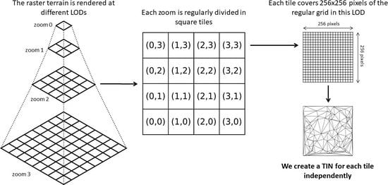


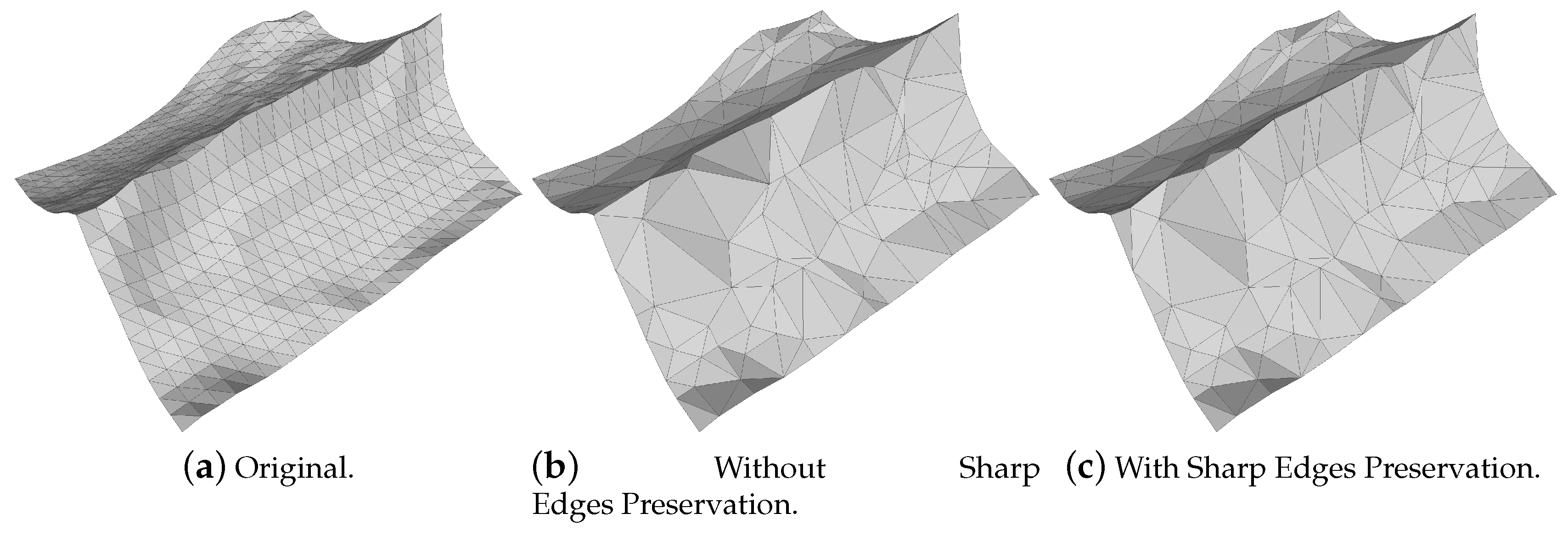