Article

PolSAR Image Classification with Lightweight 3D Convolutional Networks

Department of Information Engineering, Harbin Institute of Technology, Harbin 150001, China
*
Author to whom correspondence should be addressed.
Remote Sens. 2020, 12(3), 396; https://doi.org/10.3390/rs12030396
Submission received: 22 December 2019 / Revised: 16 January 2020 / Accepted: 21 January 2020 / Published: 26 January 2020

Abstract

:
Convolutional neural networks (CNNs) have become the state-of-the-art in optical image processing. Recently, CNNs have been used in polarimetric synthetic aperture radar (PolSAR) image classification and obtained promising results. Unlike optical images, the unique phase information of PolSAR data expresses the structure information of objects. This special data representation makes 3D convolution which explicitly modeling the relationship between polarimetric channels perform better in the task of PolSAR image classification. However, the development of deep 3D-CNNs will cause a huge number of model parameters and expensive computational costs, which not only leads to the decrease of the interpretation speed during testing, but also greatly increases the risk of over-fitting. To alleviate this problem, a lightweight 3D-CNN framework that compresses 3D-CNNs from two aspects is proposed in this paper. Lightweight convolution operations, i.e., pseudo-3D and 3D-depthwise separable convolutions, are considered as low-latency replacements for vanilla 3D convolution. Further, fully connected layers are replaced by global average pooling to reduce the number of model parameters so as to save the memory. Under the specific classification task, the proposed methods can reduce up to 69.83% of the model parameters in convolution layers of the 3D-CNN as well as almost all the model parameters in fully connected layers, which ensures the fast PolSAR interpretation. Experiments on three PolSAR benchmark datasets, i.e., AIRSAR Flevoland, ESAR Oberpfaffenhofen, EMISAR Foulum, show that the proposed lightweight architectures can not only maintain but also slightly improve the accuracy under various criteria.

Graphical Abstract

1. Introduction

Polarimetric synthetic aperture radar (PolSAR), as one of the most advanced detectors in the field of remote sensing, can provide rich target information in all-weather and all-time. In recent years, more and more attention has been paid to the development of PolSAR information extractions due to the good properties of PolSAR systems. Especially, PolSAR image classification has been extensively studied as the basis of PolSAR image interpretation.
Deep learning [1] has made remarkable progress in natural language processing and computer vision, and it has the potential to be applied in many other fields. Convolutional neural networks (CNNs), as one of the representative methods of deep learning, have shown strong abilities in the task of image processing [2]. It has been proved that CNNs can obtain more abstract feature representations than traditional hand-engineered filters. The generalization performance of machine learning-based image classification algorithms has been greatly improved with the rise of CNNs. Big data, advanced algorithms, and improvements in computing power are the key factors for the success of CNNs. These factors also exist in PolSAR image classification. Therefore, it is promising to use CNNs to improve PolSAR image classification.
Before the popularity of deep learning, machine learning algorithms have been applied in PolSAR image classification for a long time. Statistical machine learning methods represented by support vector machines have been utilized to implement PolSAR image feature classification [3]. Considering the significant achievements made by CNNs, many studies have applied CNNs to the task of SAR or PolSAR image classification and achieved remarkable results [4]. Ding et al. introduced a four-layers CNN architecture [5] to do SAR image target recognition for the first time. A more carefully-designed network architecture was proposed to further explore deep features [6]. The impact of target angles was taken into consideration, and a multi-view metric based CNN was proposed to achieve high precision classification on MSTAR dataset [7]. Ren et al. introduced a patch-sorted based architecture for high-resolution SAR image classification [8]. Some complex tasks were implemented on the basis of deep features extracted by CNNs, such as change detection [9] and road segmentation [10]. In contrast, the application level of CNNs in PolSAR image classification is lower, but it is in the stage of rapid development. After some attempts on stacking shallow models [11], Zhou et al. applied CNN to PolSAR image classification for the first time [12]. In their work, a three-layers architecture was introduced to classify PolSAR images and obtained promising classification results. After that, many CNN architectures were introduced such as graph-based architecture [13], fully convolutional networks [14] and some advanced network backbones [15,16]. However, due to different imaging mechanisms, directly following the architectures of optical image classification may not fully utilize the capabilities of CNNs in PolSAR image classification. In other words, CNNs still have the potential to be explored in the task of PolSAR image classification.
As mentioned above, designing suitable CNN architectures for PolSAR image classification is necessary to pursue more powerful performances. Related studies are being carried out and they can be roughly divided into two parts according to their focus, i.e., task characteristics and data form. Lack of supervision information is a representative task characteristic of PolSAR image classification. Although the acquisition of PolSAR images is not difficult, they do not have labels. In other words, most of the acquired PolSAR images cannot be directly used by the existing mainstream CNNs. Moreover, it is more difficult to label them manually compared with optical images. To handle this problem, weakly supervised methods, such as automatic pseudo-labels, transfer learning, and regularization techniques, were introduced to achieve PolSAR image small sample classification. A super-pixel restrained network was designed to do semi-supervised PolSAR classification with the aid of a pseudo-labels strategy [17]. Similarly, active learning was used to do pseudo labels and deep learning-based semi-supervised PolSAR classification was achieved in [18]. Wu et al. implemented transfer learning on a modified U-Net [19] to realize PolSAR small sample pixel-wise classification. Bi et al. added a graph-based regularization term to the ordinary CNN and achieved semi-supervised PolSAR classification [13]. In addition to improving the CNN architectures according to the characteristics of PolSAR classification tasks, making the architectures adapt to the complex-valued PolSAR data has also been extensively considered. Different from optical sensors, PolSAR can obtain the phase information between target and radar because of its unique scattering imaging mechanism. Therefore, the architectures which can make full use of the information contained in PolSAR data are of great significance to the development of CNNs in PolSAR image classification. This is also the objective of this work. Chen et al. tried to use the hand-engineered features as the input of CNNs to make better use of PolSAR data without changing the network architecture [20]. Different from changing the inputs, An intuitive improvement to better utilize complex-valued PolSAR data was extending the real-valued architectures to the complex domain [21,22]. Zhang et al. elaborated on the previous studies in detail and designed a three-layers complex-valued CNN to adapt to the characteristics of PolSAR data and implement PolSAR image classification [23]. At present, complex-valued architectures have been followed by many studies. Shang et al. introduced a complex-valued convolutional autoencoder network for PolSAR classification [24]. Complex-valued fully convolutional networks were proposed in [25] to do PolSAR semantic segmentation. Sun et al. proposed a complex-valued generative adversarial network for semi-supervised PolSAR classification [26]. However, the development of complex-valued architectures is still in its infancy. To avoid complex operations, Liu et al. attempted to learn the feature of phase independently [27]. A two-stream architecture was proposed to extract features from amplitude and phase respectively with the aid of a multi-task feature fusion mechanism [28]. It is worth noting that PolSAR covariance matrix has been used as the input of CNNs in most studies [12,15,16,23,
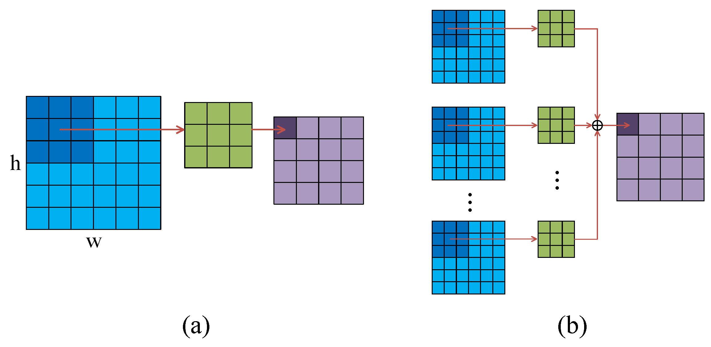
28], and the phase information is hidden between the input channels when each element of the upper triangle of PolSAR covariance matrix is regarded as a channel of the input. Recent works have revealed that, with the aid of 3D operations, channel-wise correlations can be plugged in as an additional dimension of convolution kernels to solve the problem of feature mining on special data (e.g., videos) [29,30]. Such improvements induce considerable advantages when processing PolSAR data by CNNs. Zhang et al. introduced 3D operations for the first time to implement PolSAR classification [31], which effectively improved the performance of ordinary 2D-CNNs. Tan et al. integrated complex-valued and 3D operations, and proposed a complex-valued 3D-CNN for PolSAR classification [32]. However, the performance improvement brought by 3D convolutions is based on greatly increased model parameters [30]. A large number of model parameters limit the speed of classification, which hinders the practical implementations of 3D-CNNs and the development of real-time interpretation systems [33]. Lightweight alternatives of 3D convolutions, e.g., pseudo-3D convolution [34] and depthwise separable convolution [35,36] are good means to solve this dilemma.
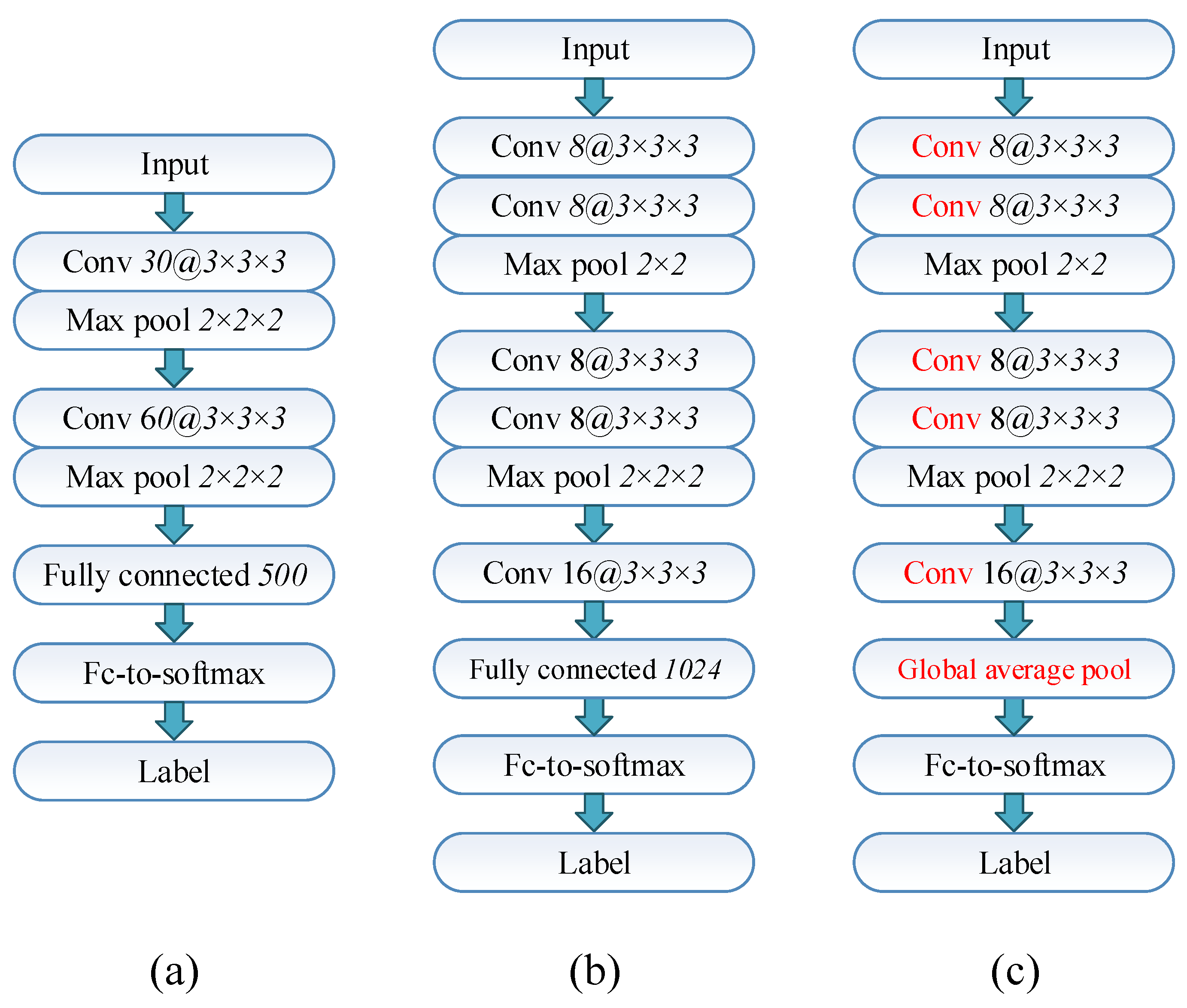
Based on the above analysis, the objective of this work is to find 3D-CNNs architectures with low computational cost as well as competitive performance for PolSAR image classification. It can be observed that almost all model parameters of a CNN exist in the convolution and fully connected layers. For these two key components, lightweight strategies are developed in this paper to compress the network architecture so as to reduce the model complexity of 3D-CNNs. Firstly, pseudo-3D convolution-based CNN (P3D-CNN) is introduced which replaces the convolution operations of 3D-CNNs by pseudo-3D convolutions. P3D-CNN uses two successive 2D operations to approximate the features extracted by 3D-CNNs. In addition, 3D-depthwise separable convolution-based CNN (3DDW-CNN) is proposed in parallel. Different from P3D-CNN, 3DDW-CNN decouples the spatial-wise and channel-wise operations that were previously mixed together to find more effective features than 3D-CNNs. The number of model parameters contained in convolution layers can be greatly reduced in the proposed two lightweight architectures. Moreover, fully connected layers of the above two architectures are eliminated and replaced by global average pooling layers [37]. This measure reduces more than 90 % of the model parameters in 3D-CNNs and greatly improves the computational efficiency. The dropout mechanism [38] is configured in the proposed architectures to further prevent over-fitting. The proposed architectures can be summarized as a lightweight 3D-CNN framework, which has more efficient convolution and fully connected operations. The proposal has inspirations for the development of many other lightweight architectures. The number of trainable parameters and the computational complexity of the involved models are compared and analyzed, which illustrates the superiority of the lightweight architectures. The classification performance of the proposed methods is tested on three PolSAR benchmark datasets. Experimental results show that considerable accuracy can be maintained by the proposed methods. The main contribution of this paper can be summarized as follows:
  • Two lightweight 3D-CNN architectures are introduced for the fast PolSAR interpretation speed during testing.
  • Two lightweight 3D convolution operations, i.e., pseudo-3D and 3D-depthwise separable convolutions, and global average pooling are applied to reduce the redundancy of 3D-CNNs.
  • A lightweight 3D-CNN framework can be summarized. Compared with ordinary 3D-CNNs, the architectures under the framework have fewer model parameters and lower computational complexity.
  • The performance of the lightweight architectures is verified on three PolSAR benchmark datasets.
The rest of this paper is organized as follows. In Section 2, the background of vanilla convolutions and their variants are introduced. The proposed methods are introduced in Section 3. The experimental results and analysis are presented in Section 4. The conclusion is discussed in Section 5.

2. Related Works

In this section, 2D convolution, 3D convolution and its lightweight versions, i.e., pseudo-3D convolution and 3D-depthwise separable convolution, are briefly analyzed. Formula expressions are avoided and graphical illustrations are used to facilitate understanding.

2.1. Vanilla Convolutions

2D convolution is the choice of most CNNs, which can be used to extract the information from the input maps. The process of vanilla 2D convolution operation is shown in Figure 1, from which one can see that the output of a 2D convolution is always two-dimensional, i.e., one feature map, for any size of inputs. Therefore, 2D convolution can only extract spatial information, and it is not conducive to process the data which has a relationship between channels by 2D convolutions.
Vanilla 3D convolution (C3D) can be seen as an intuitive extension of 2D convolutions and a dimension is added to extract more information [30]. As shown in Figure 1, the process of vanilla 2D convolution can be expressed as
z ( t , h ) = i = 1 k h k w x i ( t ) y i ( h ) + b ( h ) ,
where t and h mean the tth sliding window and the hth convolution kernel, k h and k w represent the spatial kernel size, x ( t ) and z ( t ) denote the tth input and the tth output, and y ( h ) and b ( h ) denote the hth kernel matrix and its bias. Similarly, C3D can be expressed as
z ( t , h ) = j = 1 k d i = 1 k h k w x i , j ( t ) y i , j ( h ) + b ( h ) ,
where k d represents the depth of kernels. The process of C3D can be seen from Figure 2, where the extra depth dimension is added to the 2D convolution kernels. The difference between 2D and 3D convolutions can be seen by comparing Figure 1b with Figure 2a. Similar to 2D convolutions to maintain the spatial size of the inputs, the size of the depth dimension is maintained through 3D convolutions. In other words, the input is only manipulated spatially for 2D convolutions and the output is always maps. However, C3D extract features from spatial and depth dimensions at the same time, and outputs cubes. The latter undoubtedly contains more information as well as more model parameters to be trained.

2.2. Pseudo-3D Convolution

The process of pseudo-3D convolution (P3D) can be seen in Figure 3. Two successive sub-operations work on spatial dimension and depth dimensions respectively are used by P3D to simulate the effect of C3D. It has been proven that P3D can greatly reduce the number of trainable parameters while keeping accuracy [34].
As shown in Figure 3, P3D decomposes the k × k × k C3D kernel into k × k × 1 and 1 × 1 × k . The number of model parameters of each kernel is reduced from k 3 to k ( k + 1 ) . Such divide-and-conquer heuristic modeling ideas are familiar and usually effective [35,39,40]. Intuitively, assigning clear task requirements to convolution operations can increase their productivity. Therefore, compared with C3D, P3D can not only reduce the number of model parameters but also slightly improve accuracy.

2.3. 3D-Depthwise Separable Convolution

The simultaneous existence of multiple convolution kernels provides a guarantee for the powerful feature extraction capability of CNNs. In fact, the feature maps extracted by multiple convolution kernels can be regarded as many different kinds of features [41]. However, from the comparison of the two sub-graphs in Figure 1, multiple groups of convolution kernels have brought about several times of parameters. Depthwise separable convolution [35] was proposed as an effective way to reduce the increasing of parameters in this case, which realized a very efficient replacement by decoupling the spatial and channel-wise operations of the vanilla 2D convolution. For an h × w × c input map, 2D convolution kernels with the size of k × k × c × c are required to produce the output with the size of h × w × c (performing the operation in Figure 1b c times with zero-padding). However, the convolution kernels with the size of k × k × c × 1 + 1 × 1 × c × c are needed for depthwise separable convolution to achieve the same effect. Due to the good performance of depthwise separable convolution in 2D tasks, it is a natural idea to extend it to 3D tasks. A similar idea has also been considered in [36].
The improved strategy is straightforward, that is, replacing the 2D convolutions in 2D-depthwise separable convolution with 3D operations. The comparison between C3D and 3D-depthwise separable convolution is shown in Figure 4. It can be seen from Figure 4a that c times C3D operations are implemented (different colors represent different groups of filters) to generate c numbers of 3D feature cubes. The process of 3D-depthwise separable convolution is shown in Figure 4b. Similar to 2D operations, 3D-depthwise separable convolution can also be divided into depthwise and pointwise operations. The kernels of 3D depthwise convolution are shown in the second column in Figure 4b, and 3D pointwise convolution kernels are shown as the fourth column. Obviously, the idea of depthwise separable convolution is inherited, and an extra dimension is added to implement 3D feature extraction. k × k × k × c × c numbers of model parameters are needed in Figure 4a, and they can be decomposed into c times 3D depthwise convolution with the parameters of k × k × k and c times 3D pointwise convolution with the parameters of 1 × 1 × 1 × c . Therefore, the model complexity can be greatly reduced, which makes it possible to be utilized with limited resources.

3. Proposed Methods

In this section, the representation of PolSAR images is present firstly. PolSAR coherence matrix T is adopted as the starting point in this work. Then the implementation details of the proposed architectures are introduced.

3.1. Representation of PolSAR Images

A polarized scattering matrix can fully characterize the electromagnetic scattering properties of ground targets. The scattering matrix is defined as:
S = S H H S H V S V H S V V ,
where S P Q ( P , Q { H , V } ) represents the backscattering coefficient of the polarized electromagnetic wave in emitting Q direction and receiving P direction. H and V represent the horizontal and vertical polarization, respectively. According to the reciprocity theorem, the S matrix satisfies S H V = S V H . To describe the scattering properties of targets more clearly, the S matrix is usually transformed into the polarization coherence matrix or polarization covariance matrix. The polarization vector and coherence matrix based on Pauli decomposition are expressed as (4) and (5)
k = 1 2 [ S H H + S V V , S H H S V V , 2 S H V ] T ,
[ T ] = k k H .
The polarization coherence matrix T is a Hermitian matrix, and all its elements except the diagonal element, are complex numbers. Generally, the upper triangular elements [ T 11 , T 12 , T 13 , T 22 , T 23 , T 33 ] are taken and divided into their real and imaginary parts as the input of CNNs. At this point, there are nine real-valued numbers to describe each pixel of PolSAR images.

3.2. Lightweight 3D-CNNs for PolSAR Classification

Data preprocessing, model design, and network training and testing are generally included steps of the CNNs-based PolSAR classification methods, as shown in Figure 5.
In this work, the steps of classification can be summarized as follows: (1) Labeled image slices with the size of 15 × 15 are cut around the central pixel according to the source data of PolSAR image (polarization coherence matrix is used in this work) and the ground truth map. (2) The training set, validation set, and testing set can be obtained from the labeled samples. (3) A tailored CNN architecture is designed according to the characteristics of PolSAR data. (4) The architecture is trained and saved on the training and validation sets, and then tested on the testing set. (5) Each sample of the original data is input to the neural network and the interpretation results of the whole map can be obtained. In most cases, the construction of the CNN architecture is the central part. Some available architectures can be seen in Figure 6.
The original 3D-CNN architecture used for PolSAR image classification [31] is shown in Figure 6a. Compared to their work, a deeper architecture can be seen in Figure 6b, in which the updated network has three additional convolution layers and the network width is reduced to alleviate the adverse effects of the increase of depth. Such a 3D architecture can not only mine the spatial relations but also explore the correlations between different elements of the polarization coherence matrix so as to extract more comprehensive information. Therefore, this architecture is chosen to be the backbone of this paper. It is worth noting that building the network backbone is not the objective of this paper, but to compare the proposed lightweight methods with the ordinary ones in a fair environment. Although 3D-CNNs showed a promising performance [31], it also brought a slower interpretation speed due to more model parameters and higher complexity. The computational difficulty mainly centers on the convolution and fully connected layers for the architecture in Figure 6b. Thus, the lightweight improvements designed for these two parts are implemented.
The C3D operations of 3D-CNNs are replaced with the two former introduced lightweight convolution operations to reduce the computational complexity of the convolution layer. It can be seen from Figure 6c that only the way the convolutions is changed, without modifying their depth, width, and kernel size. It can be easily proven that the lightweight convolution layers contain a similar number of model parameters as the 2D layers, and only half or even less of the C3D layers. A more detailed analysis of the changes in the number of model parameters will be given later.
In the architecture shown in Figure 6a, the data is expanded into a 1D vector and enters the fully connected layers when the processing of convolutions is finished. The role of fully connected layers is to reduce the dimension of the outputs of convolution layers. Results of the fully connected layers will be activated by softmax activation to achieve feature classification, which can be defined as
σ s o f t m a x ( x i ) = e x i j e x j ,
where σ s o f t m a x ( x ) means the softmax activation of the input x, i denotes the ith category, and j is the number of categories. Thus, a j × 1 vector whose element represents the probability of belonging to the corresponding category can be obtained as the final prediction.
Improvements to the fully connected layer have been concerned a lot because it occupies more than 90 % model parameter of CNNs. Global average pooling (GAP) has been proved that it can be seen as a plug-and-play replacement for fully connected layers to save the computational resource [37]. As can be seen from Figure 7a, m × m three-channels 2D feature maps are flattened to a vector as the input of fully connected layers. When the number of the category is J and the hidden node of the fully connected layers is H, the total number of parameters is ( m × m × 3 × H ) + ( H × J ) for the two fully connected layers. When the input becomes multi-channel 3D features, the large amount of parameters are multiplied by the depth of features. Such a large number of parameters not only brings computational difficulties but also increases the risk of over-fitting. In the proposed architectures, spatial global average pooling is performed as shown in Figure 7b. For each channel of the output feature cube, the process of the used GAP can be defined as
y ( d ) = f g a p ( x ( d ) ) = 1 h × w h w x h , w ( d ) ,
where x and y represent the input and output of the GAP layer. d denotes the depth of the feature cube, and h and w represent its height and width. The above operations are performed on each channel for the multi-channel input 3D feature cubes, which can greatly reduce the number of model parameters so as to cut down the computational cost.

4. Experiments

In this section, to evaluate the performance of the proposed methods, they are tested on three PolSAR benchmark datasets and compared with several alternatives. The experimental environment uses a PC with Intel Core i7-7700 CPU with 16 GB RAM. A deep learning toolbox [42] is utilized to minimize the difficulty of algorithm implementation.

4.1. Datasets and Settings

Three widely-used PolSAR benchmark datasets are employed in the experiments: AIRSAR Flevoland, ESAR Oberpfaffenhofen, and EMISAR Foulum. Figure 8, Figure 9 and Figure 10 show their Pauli maps and ground truth maps, respectively.

4.1.1. AIRSAR Flevoland

As shown in Figure 8, an L-band, full polarimetric image of the agricultural region of the Netherlands is obtained through NASA/Jet Propulsion Laboratory AIRSAR [43]. The size of this image is 750 × 1024 and the spatial resolution is 0.6 m × 1.6 m. The ground truth map is shown in Figure 8b, which is adapted from [44]. There are 15 kinds of ground objects including buildings, rapeseed, beet, stem beans, peas, forest, lucerne, potatoes, bare soil, grass, barley, water, and three kinds of wheat, and a total of 184,592 image slices are contained in this dataset. The details of each category are shown in Table 1.

4.1.2. ESAR Oberpfaffenhofen

An L-band, full polarimetric image of Oberpfaffenhofen, Germany, 1200 × 1300 scene size, are obtained through the ESAR airborne platform [43]. Its Pauli color-coded image and ground truth map can be seen in Figure 9. The ground truth map is adapted from [45]. According to the ground truth, each pixel in the map is divided into three categories: built-up areas, wood land, and open areas, except for some unknown regions. A total of 1,307,142 image slices are contained in this dataset. The details of each category are shown in Table 2.

4.1.3. EMISAR Foulum

The last full polarimetric image used in this experiment is the L-band image taken by EMISAR in Foulum, Denmark. EMISAR is a full polarized airborne SAR operating in L and C bands with a resolution of 2 m × 2 m and mainly acquired and studied by Danish Center for Remote Sensing (DCRS). Figure 10 shows its Pauli RGB image and ground truth map. The size of this image is 1000 × 1750 . The calibration of the terrains in Figure 10b refers to [46,47], and each pixel in the map is divided into seven categories: lake, buildings, forest, peas, winter rape, winter wheat, and beet. There are 431,088 image slices in this dataset. The details of each category are shown in Table 3.

4.2. Experiments Starting

To validate the significance of the proposed PolSAR image classification framework, ordinary CNN (CNN), 2D-depthwise separable convolution CNN (DW-CNN) and C3D CNN (3D-CNN) are chosen to be compared. Their architectures and hyperparameters are set as Figure 6b except for the way of convolution. The proposed two classifiers are denoted as P3D-CNN and 3DDW-CNN for convenience. During the training and testing, the size of kernels are 3 × 3 for 2D convolutions and 3 × 3 × 3 for 3D convolutions. The dropout rate is 0.8 for fully connected layers. An improved stochastic gradient descent optimization method [48] is chosen to train the involved architectures with the learning rate of 0.001 .
To evaluate the performance of the algorithms mentioned in this paper, the overall accuracy (OA) and kappa coefficient (Kappa) [49] are chosen as criteria, which can be defined as follows:
O A = i = 1 c M i i = 1 c N i
where c is the number of categories. M i and N i denote the number of correctly classified categories and the total number of ith categories, respectively.
K a p p a = O A P 1 P , w i t h P = 1 n 2 i = 1 c H ( i , : ) H ( : , i )
where n is the number of testing samples and H denotes the classification confusion matrix.
The number of training epoch is important which determines whether the model converges or not. 9000 and 4500 samples of the AIRSAR Flevoland dataset, and 7000 and 3500 samples of the EMISAR Foulum dataset are randomly chosen without overlaps as training and validation sets. Then experiments of 3D-CNN are carried out to find a suitable value of training epoch. The experimental results are shown in Figure 11.
One can see from the experimental results that the training accuracy tends to be stable after 100 iterations and the validation accuracy does not change much after 200 iterations. Combined with these two points, the value of the epoch is set to 250 in the experiments to ensure convergence.When the training epoch reaches the upper limit, the model with the highest OA on the validation set should be selected as the final trained model to ensure the stability of the training process.
The size of the training set also needs to be carefully considered. We do comparative experiments to find an appropriate number of training samples in order to save memory as much as possible under the premise of guaranteeing the training effects. In the experiments, we randomly extract a certain number of samples (the latter size is twice as large as the former for easy analysis) from each category of labeled samples to form the training set. Two basic models including CNN [12] and 3D-CNN [31] are tested on different training sets of three benchmarks. One thing can be found that the number of buildings category is small, so in the experiments on the AIRSAR dataset, the number of training samples is fixed to 600 for buildings when the extracted number is more than 600. The experimental results are listed in Table 4, from which we can see that when the scale of the training set moves from small to large, the accuracy of both the CNN and 3D-CNN shows an upward trend. Results on the AIRSAR and EMISAR datasets show that this upward trend eases when the number of training samples of each category exceeds 1200 and 4000. Although the large size of the training set brings a slight improvement for the ESAR dataset, 1000 samples per category met our needs. After obtaining the training set, half of the training set were extracted from the remaining samples to form the validation set, and 30% of the remaining were taken as the testing set.

4.3. Results and Comparisons

Under the experimental environment and settings described earlier, the classification results of different methods are shown in Figure 12, Figure 13 and Figure 14, and the accuracies are listed in Table 5, Table 6 and Table 7, respectively. Generally, the proposed methods achieve better performance than the compared ones. The experimental results on the AIRSAR Flevoland dataset can be seen from Table 5 and the classification results of the whole map are listed in Figure 12.
The results in Table 5 prove that the proposed methods slightly improve the classification accuracy on this data set. From the experimental results, it can be seen that 3D networks have a better performance than 2D networks, which confirms the importance of 3D convolutions for the PolSAR classification. Furthermore, it can be seen that the OA and Kappa of lightweight 3D convolution-based methods are higher and ordinary 3D-CNN, especially in the identification of the rapeseed and wheat categories. This shows that there is potential redundancy in C3D operations and the lightweight strategies can improve not only the computational efficiency but also the classification performance.
Whole map classification results can be seen in Figure 12, it can be seen that the proposed methods have more powerful capabilities for distinguishing between forest and grass. In addition, apart from rapeseed and three types of wheat, the proposed methods are also effective for classifying beet and potatoes.
The experimental results on ESAR Oberpfaffenhofen can be seen from Table 6 and the classification results of the whole map are listed in Figure 13. On this data set, the analysis results are generally consistent with the previous ones. The 3D models achieve better results than the 2D models under different criteria. In these experiments, 3DDW-CNN achieves the best performance. It has a 1.37 % improvement of OA and 2.04 % improvement of kappa compared with the ordinary 3D-CNN. The P3D-based model also achieves a several signs of progress. Similar conclusions under different datasets also confirm the generalization performance of the proposed methods.
The results overlaid with the ground truth map on ESAR Oberpfaffenhofen are shown in Figure 13, where it can be seen that serious confusions exist between built-up areas and woodlands for 2D models. This phenomenon has been weakened in 3D-CNN, and the proposed methods further alleviate this problem. In addition, compared with other methods, the proposed methods have more complete and pure classification results for the open areas.
The experimental results on the EMISAR Foulum can be seen from Table 7 and the classification results of the whole map are listed in Figure 14. Compared with the former two datasets, EMISAR Foulum data which contains quite complex terrain information is not so widely used. Similar conclusions can be drawn from the analysis of the experimental results shown in Table 7, where the proposed P3D-CNN achieves the best classification results. It is worth pointing out that although the results of 3DDW-CNN is slightly lower than 3D-CNN, such a small performance degradation (about 0.03 % ) is acceptable under the premise of reducing computational complexity.
One can see from Figure 14 that the following groups of objects are easy to be misclassified, including lake-peas, peas-winter wheat, buildings-forest. The proposed methods show competitive performance when generally solving the above problems, although the results of P3D-CNN for the lake is not very good.

4.4. Studies of Complexity

In previous experiments, the classification performance of the proposed methods have been verified. In this part, we analyze the number of trainable parameters and the computational complexity of the proposed methods. An intuitive comparison of the number of trainable parameters and overall accuracy of the involved models on the AIRSAR Flevoland dataset can be seen in Table 8.
As can be seen from Table 8, P3D-CNN contains half of the parameters of 3D-CNN in convolution layers, which is 1.44 times that of 2D-CNN. 3DDW-CNN is even lighter, which cuts about 70 % trainable parameters in convolution layers of 3D-CNN. As the GAP is introduced to replace the fully connected layer, the total parameters contained in the model are greatly reduced. Meanwhile, the proposed two methods not only maintain the accuracy of 3D-CNN but also improve slightly.
Furthermore, the value of the floating point operations (FLOPs) in the convolution layers of each method is calculated, which is a popular evaluation metric to compare the complexity of algorithms. FLOPs in convolution layers of the proposed and comparing methods are calculated. Then the comparison combining accuracy and complexity can be seen from Figure 15, in which the x-axis represents the value of convolution FLOPs, and the y-axis represents the overall accuracy. Four involved methods, i.e., CNN, two proposed ones, and 3D-CNN, are shown in the figure from the left to the right. Each one has three bars, which represent its OA on the three different datasets. It can be seen that the proposed methods, i.e., the middle two of the four columns, not only have lower FLOPs, but also improve the classification accuracy slightly than 3D-CNN (the rightmost column). This result can verify the theoretical analysis.

5. Conclusion

Inspired by the recent lightweight improvements for deep neural networks, in this paper, two lightweight 3D-CNN architectures are proposed for PolSAR image classification. Lightweight 3D convolutions, i.e., pseudo-3D and 3D-depthwise separable convolutions, are introduced to perform feature extraction and reduce the redundancy of 3D convolutions. Meanwhile, global average pooling is introduced to replace the fully connected layer considering the huge number of model parameters contained in it. In this way, over 90 % model parameters of 3D-CNNs can be compressed so as to support the high-precision interpretation under the resource-constrained system. Moreover, a general lightweight 3D-CNN framework can be summarized, which can help future research. Such a PolSAR tailored classification framework can not only improve the running speed but also boost the performance of convolutions. Experimental results on three PolSAR benchmark datasets show that the proposed architectures have promising classification performance and low computational complexity. In the future, complex-valued CNN architectures, weakly-supervised classification methods and finding the optimal hyperparameters automatically are all issues we are considering.

Author Contributions

All the authors made significant contributions to this work. H.D. and L.Z. devised the approach and wrote the paper. H.D. conducted the experiments and analyzed the data. Supervision and suggestions, L.Z. and B.Z.; writing—review and editing, B.Z. All authors have read and agreed to the published version of the manuscript.

Funding

This work was supported in part by the National Natural Science Foundation of China (61401124, 61871158), in part by Scientific Research Foundation for the Returned Overseas Scholars of Heilongjiang Province (LC2018029), in part by Aeronautical Science Foundation of China (20182077008).

Conflicts of Interest

The authors declare no conflicts of interest.

References

  1. LeCun, Y.; Bengio, Y.; Hinton, G. Deep learning. Nature 2015, 521, 436–444. [Google Scholar] [CrossRef]
  2. Krizhevsky, A.; Sutskever, I.; Hinton, G. ImageNet classification with deep convolutional neural networks. In Proceedings of the Advances in Neural Information Processing Systems (NIPS), Lake Tahoe, NV, USA, 3–6 December 2012; pp. 1097–1105. [Google Scholar] [CrossRef]
  3. Lardeux, C.; Frison, P.; Tison, C.; Souyris, J.; Stoll, B.; Fruneau, B.; Rudant, J. Support vector machine for multifrequency SAR polarimetric data classification. IEEE Trans. Geosci. Remote Sens. 2009, 47, 4143–4152. [Google Scholar] [CrossRef]
  4. Zhu, X.; Tuia, D.; Mou, L.; Xia, G.; Zhang, L.; Xu, F.; Fraundorfer, F. Deep learning in remote sensing: A comprehensive review and list of resources. IEEE Geosci. Remote Sens. Mag. 2017, 5, 8–36. [Google Scholar] [CrossRef] [Green Version]
  5. Ding, J.; Chen, B.; Liu, H.; Huang, M. Convolutional neural network with data augmentation for SAR target recognition. IEEE Geosci. Remote Sens. Lett. 2016, 13, 364–368. [Google Scholar] [CrossRef]
  6. Chen, S.; Wang, H.; Xu, F.; Jin, Y. Target classification using the deep convolutional networks for SAR images. IEEE Trans. Geosci. Remote Sens. 2016, 54, 4806–4817. [Google Scholar] [CrossRef]
  7. Pei, J.; Huang, Y.; Huo, W.; Zhang, Y.; Yang, J.; Yeo, T. SAR automatic target recognition based on multiview deep learning framework. IEEE Trans. Geosci. Remote Sens. 2017, 56, 2196–2210. [Google Scholar] [CrossRef]
  8. Ren, Z.; Hou, B.; Wen, Z.; Jiao, L. Patch-sorted deep Feature Learning for high resolution SAR image classification. IEEE J. Sel. Top. Appl. Earth Obs. Remote Sens. 2018, 11, 3113–3126. [Google Scholar] [CrossRef]
  9. Gong, M.; Zhao, J.; Liu, J.; Miao, Q.; Jiao, L. Change detection in synthetic aperture radar images based on deep neural networks. IEEE Trans. Neural Netw. Learn. Syst. 2016, 27, 125–138. [Google Scholar] [CrossRef]
  10. Corentin, H.; Azimi, S.; Merkle, N. Road segmentation in SAR satellite images with deep fully convolutional neural networks. IEEE Geosci. Remote Sens. Lett. 2018, 15, 1867–1871. [Google Scholar] [CrossRef] [Green Version]
  11. Jiao, L.; Liu, F. Wishart deep stacking network for fast PolSAR image classification. IEEE Trans. Image Process. 2016, 25, 3273–3286. [Google Scholar] [CrossRef]
  12. Zhou, Y.; Wang, H.; Xu, F.; Jin, Y. Polarimetric SAR image classification using deep convolutional neural networks. IEEE Geosci. Remote Sens. Lett. 2017, 13, 1935–1939. [Google Scholar] [CrossRef]
  13. Bi, H.; Sun, J.; Xu, Z. A graph-based semisupervised deep learning model for PolSAR image classification. IEEE Trans. Geosci. Remote Sens. 2019, 57, 2116–2132. [Google Scholar] [CrossRef]
  14. Yan, W.; Chu, H.; Liu, X.; Liao, M. A hierarchical fully convolutional network integrated with sparse and low-rank subspace representations for PolSAR imagery classification. Remote Sens. 2018, 10, 342. [Google Scholar] [CrossRef] [Green Version]
  15. De, S.; Bruzzone, L.; Bhattacharya, A.; Bovolo, F.; Chaudhuri, S. A novel technique based on deep learning and a synthetic target database for classification of urban areas in PolSAR data. IEEE J. Sel. Top. Appl. Earth Obs. Remote Sens. 2018, 11, 154–170. [Google Scholar] [CrossRef]
  16. Dong, H.; Zhang, L.; Zou, B. Densely connected convolutional neural network based polarimetric SAR image classification. In Proceedings of the IEEE International Geoscience and Remote Sensing Symposium (IGARSS), Yokohama, Japan, 28 July–2 August 2019; pp. 3764–3767. [Google Scholar] [CrossRef]
  17. Geng, J.; Ma, X.; Fan, J.; Wang, H. Semisupervised classification of polarimetric SAR image via superpixel restrained deep neural network. IEEE Geosci. Remote Sens. Lett. 2018, 15, 122–126. [Google Scholar] [CrossRef]
  18. Bi, H.; Xu, F.; Wei, Z.; Xue, Y.; Xu, Z. An active deep learning approach for minimally supervised PolSAR image classification. IEEE Trans. Geosci. Remote Sens. 2019, 57, 9378–9395. [Google Scholar] [CrossRef]
  19. Ronneberger, O.; Fischer, P.; Brox, T. U-Net: Convolutional networks for biomedical image segmentation. arXiv 2015, arXiv:1505.04597. [Google Scholar]
  20. Chen, S.; Tao, C. PolSAR image classification using polarimetric-feature-driven deep convolutional neural network. IEEE Geosci. Remote Sens. Lett. 2018, 15, 627–631. [Google Scholar] [CrossRef]
  21. Hänsch, R. Complex-valued multi-layer perceptrons-An application to polarimetric SAR data. Photogramm. Eng. Remote Sens. 2010, 76, 1081–1088. [Google Scholar] [CrossRef]
  22. Hänsch, R.; Hellwich, O. Complex-valued convolutional neural networks for object detection in PolSAR data. In Proceedings of the 8th European Conference on Synthetic Aperture Radar (EUSAR), Aachen, Germany, 7–10 June 2010; pp. 1–4. [Google Scholar]
  23. Zhang, Z.; Wang, H.; Xu, F.; Jin, Y. Complex-valued convolutional neural network and its application in polarimetric SAR image classification. IEEE Trans. Geosci. Remote Sens. 2017, 55, 7177–7188. [Google Scholar] [CrossRef]
  24. Shang, R.; Wang, G.; Michael, A.; Jiao, L. Complex-valued convolutional autoencoder and spatial pixel-squares refinement for polarimetric SAR image classification. Remote Sens. 2019, 11, 522. [Google Scholar] [CrossRef] [Green Version]
  25. Cao, Y.; Wu, Y.; Zhang, P.; Liang, W.; Li, M. Pixel-wise PolSAR image classification via a novel complex-valued deep fully convolutional network. Remote Sens. 2019, 11, 2653. [Google Scholar] [CrossRef] [Green Version]
  26. Sun, Q.; Li, X.; Li, L.; Liu, X.; Liu, F.; Jiao, L. Semi-supervised complex-valued GAN for polarimetric SAR image classification. In Proceedings of the IEEE International Geoscience and Remote Sensing Symposium (IGARSS), Yokohama, Japan, 29 July–2 August 2019; pp. 3245–3248. [Google Scholar] [CrossRef] [Green Version]
  27. Liu, X.; Tu, M.; Wang, Y.; He, C. Polarimetric phase difference aided network for PolSAR image classification. In Proceedings of the IEEE International Geoscience and Remote Sensing Symposium (IGARSS), Valencia, Spain, 22–27 July 2018; pp. 6667–6670. [Google Scholar] [CrossRef]
  28. Zhang, L.; Dong, H.; Zou, B. Efficiently utilizing complex-valued PolSAR image data via a multi-task deep learning framework. ISPRS J. Photogramm. Remote Sens. 2019, 157, 59–72. [Google Scholar] [CrossRef] [Green Version]
  29. Ji, S.; Xu, W.; Yang, M.; Yu, K. 3D convolutional neural networks for human action recognition. IEEE Trans. Pattern Anal. Mach. Intell. 2013, 35, 221–231. [Google Scholar] [CrossRef] [Green Version]
  30. Tran, D.; Bourdev, L.; Fergus, R.; Torresani, L.; Paluri, M. Learning spatiotemporal features with 3D convolutional networks. In Proceedings of the IEEE International Conference on Computer Vision (ICCV), Santiago, Chile, 7–13 December 2015; pp. 4489–4497. [Google Scholar] [CrossRef] [Green Version]
  31. Zhang, L.; Chen, Z.; Zou, B. Polarimetric SAR terrain classification using 3D convolutional neural network. In Proceedings of the IEEE International Geoscience and Remote Sensing Symposium(IGARSS), Valencia, Spain, 22–27 July 2018; pp. 4551–4554. [Google Scholar] [CrossRef]
  32. Tan, X.; Li, M.; Zhang, P.; Wu, Y.; Song, W. Complex-valued 3-D convolutional neural network for PolSAR image classification. IEEE Geosci. Remote Sens. Lett. 2019, in press. [Google Scholar] [CrossRef]
  33. Chen, H.; Zhang, F.; Tang, B.; Yin, Q.; Sun, X. Slim and efficient neural network design for resource-constrained SAR target recognition. Remote Sens. 2018, 10, 1618. [Google Scholar] [CrossRef] [Green Version]
  34. Qiu, Z.; Yao, T.; Mei, T. Learning spatio-temporal representation with pseudo-3D residual networks. In Proceedings of the IEEE International Conference on Computer Vision (ICCV), Venice, Italy, 22–29 October 2017; pp. 5534–5542. [Google Scholar] [CrossRef] [Green Version]
  35. Chollet, F. Xception: Deep learning with depthwise separable convolutions. In Proceedings of the IEEE conference on Computer Vision and Pattern Recognition (CVPR), Honolulu, HI, USA, 21–26 July 2017; pp. 1800–1807. [Google Scholar] [CrossRef] [Green Version]
  36. Ye, R.; Liu, F.; Zhang, L. 3D depthwise convolution: Reducing model parameters in 3D vision tasks. arXiv 2018, arXiv:1808.01556. [Google Scholar]
  37. Lin, M.; Chen, Q.; Yan, S. Network in network. arXiv 2013, arXiv:1312.4400. [Google Scholar]
  38. Srivastava, N.; Hinton, G.; Krizhevsky, A.; Sutskever, I.; Salakhutdinov, R. Dropout: A simple way to prevent neural networks from overfitting. J. Mach. Learn. Res. 2014, 15, 1929–1958. [Google Scholar] [CrossRef]
  39. Simonyan, K.; Zisserman, A. Two-stream convolutional networks for action recognition in videos. arXiv 2014, arXiv:1406.2199. [Google Scholar]
  40. Xie, S.; Girshick, R.; Dollár, P.; Tu, Z.; He, K. Aggregated residual transformations for deep neural networks. In Proceedings of the IEEE conference on Computer Vision and Pattern Recognition (CVPR), Honolulu, HI, USA, 21–26 July 2017; pp. 5987–5995. [Google Scholar] [CrossRef] [Green Version]
  41. Hu, J.; Shen, L.; Sun, G. Squeeze-and-excitation networks. In Proceedings of the IEEE conference on Computer Vision and Pattern Recognition (CVPR), Salt Lake City, UT, USA, 18–22 June 2018; pp. 7132–7141. [Google Scholar] [CrossRef] [Green Version]
  42. Abadi, M.; Barham, P.; Chen, J.; Chen, Z.; Davis, A.; Dean, J.; Devin, M.; Ghemawat, S.; Irving, G.; Isard, M. TensorFlow: Large-scale machine learning on heterogeneous distributed systems. arXiv 2016, arXiv:1603.04467. [Google Scholar]
  43. Earth Online. Available online: http://envisat.esa.int/POLSARpro/datasets.html2 (accessed on 1 December 2019).
  44. Yu, P.; Qin, A.; Clausi, D. Unsupervised polarimetric SAR image segmentation and classification using region growing with edge penalty. IEEE Trans. Geosci. Remote Sens. 2012, 50, 1302–1317. [Google Scholar] [CrossRef]
  45. Liu, B.; Hu, H.; Wang, H.; Wang, K.; Liu, X.; Yu, W. Superpixel-based classification with an adaptive number of classes for polarimetric SAR images. IEEE Trans. Geosci. Remote Sens. 2013, 51, 907–924. [Google Scholar] [CrossRef]
  46. Skriver, H.; Dall, J.; Le Toan, T.; Quegan, S.; Ferro-Famil, L.; Pottier, E.; Lumsdon, P.; Moshammer, R. Agriculture classification using PolSAR data. In Proceedings of the 2nd International Workshop on POLinSAR, Frascati, Italy, 17–21 January 2005; pp. 213–218. [Google Scholar]
  47. Conradsen, K.; Nielsen, A.; Schou, J.; Skriver, H. A test statistic in the complex wishart distribution and its application to change detection in polarimetric SAR data. IEEE Trans. Geosci. Remote Sens. 2003, 41, 4–19. [Google Scholar] [CrossRef] [Green Version]
  48. Kingma, D.; Ba, J. Adam: A method for stochastic optimization. arXiv 2015, arXiv:1412.6980. [Google Scholar]
  49. Cohen, J. A coefficient of agreement for nominal scales. Educ. Psychol. Meas. 1960, 20, 37–46. [Google Scholar] [CrossRef]
Figure 1. Illustrations of vanilla 2D convolution. (a) When the input is a single h × w map, each kernel is k × k and the corresponding output is a 2D ( h k + 1 ) × ( w k + 1 ) map. (b) When the input is c numbers h × w maps, each kernel is k × k × c . Doing the same operation on each channel as in (a), getting c 2D maps and add them up. The outputs of two sub-graphs are 2D maps with the same size.
Remotesensing 12 00396 g001
Figure 2. Illustrations of vanilla 3D convolution (C3D). C3D is an intuitive extension of 2D convolution. (a) When the input is a single h × w × d cube, each kernel is k × k × k and the corresponding output is a 3D ( h k + 1 ) × ( w k + 1 ) × ( d k + 1 ) cube. (b) When the input is c numbers h × w × d cubes, each kernel is k × k × k × c . Same as the operations in (a), c numbers 3D cubes can be obtained and add them up. The outputs of two sub-graphs are 3D cubes with the same size.
Remotesensing 12 00396 g002
Figure 3. The process of pseudo-3D convolution (P3D). P3D is divided into two steps to achieve low-latency approximation to C3D, and a nonlinear activation exists between the two. (a) Step 1: Operating 2D convolution in the spatial dimension of the h × w × d input, each kernel is k × k × 1 and the corresponding output is a ( h k + 1 ) × ( w k + 1 ) × d cube. (b) Step 2: Operating 1D convolution in the depth dimension, each kernel is 1 × 1 × k . Getting the final output with the size of ( h k + 1 ) × ( w k + 1 ) × ( d k + 1 ) .
Remotesensing 12 00396 g003
Figure 4. Illustrations of C3D and 3D-depthwise separable convolution with multi groups of kernels. Different filters are coded by different colors, and the convolution kernels within the same group are marked by the same color. (a) When the number of the kernels of C3D is c. (b) The process of 3D-depthwise separable convolution in the same situation. All 2D operations in depth separable convolution are replaced by 3D operations in (b). Firstly, doing vanilla 3D convolutions on each channel of the input with the kernel size of k × k × k (3D depthwise convolution). Then, doing c times 1 × 1 × 1 convolutions to the intermediates (3D pointwise convolution), and the output with the same size of C3D can be obtained.
Remotesensing 12 00396 g004
Figure 5. General flow chart of the CNNs-based PolSAR images classification methods.
Remotesensing 12 00396 g005
Figure 6. 3D architectures for PolSAR image classification. (a) The architecture of 3D-convoluted neural networks (CNN) proposed by [31]. (b) The updated version of 3D-CNN in this paper. (c) The proposed 3D-CNN framework with lightweight 3D convolutions and global average pooling.
Remotesensing 12 00396 g006
Figure 7. An intuitive comparison between fully connected layer and global average pooling layer for multi-channel 2D input.
Remotesensing 12 00396 g007
Figure 8. AIRSAR Flevoland dataset. (a) Pauli RGB map. (b) Ground truth map.
Remotesensing 12 00396 g008
Figure 9. ESAR Oberpfaffenhofen dataset. (a) Pauli RGB map. (b) Ground truth map.
Remotesensing 12 00396 g009
Figure 10. EMISAR Foulum dataset. (a) Pauli RGB map. (b) Ground truth map.
Remotesensing 12 00396 g010
Figure 11. The influence of epoch on the performance of 3D-CNN. (a) The results on the AIRSAR Flevoland dataset. (b) The results on the EMISAR Foulum dataset.
Remotesensing 12 00396 g011
Figure 12. Classification results of the whole map on the AIRSAR Flevoland data with different methods. (a) Ground truth. (b) Result of CNN. (c) Result of depthwise separable (DW)-CNN. (d) Result of 3D-CNN. (e) Result of P3D-CNN. (f) Result of 3D-depthwise separable convolution-based CNN (3DDW-CNN).
Remotesensing 12 00396 g012
Figure 13. Classification results overlaid with the ground truth map on ESAR Oberpfaffenhofen data with different methods. (a) Ground truth. (b) Result of CNN. (c) Result of DW-CNN. (d) Result of 3D-CNN. (e) Result of P3D-CNN. (f) Result of 3DDW-CNN.
Remotesensing 12 00396 g013
Figure 14. Classification results overlaid with the ground truth map on the EMISAR Foulum data with different methods. (a) Ground truth. (b) Result of CNN. (c) Result of DW-CNN. (d) Result of 3D-CNN. (e) Result of P3D-CNN. (f) Result of 3DDW-CNN.
Remotesensing 12 00396 g014
Figure 15. Comparisons of accuracy and complexity.
Remotesensing 12 00396 g015
Table 1. Number of pixels in each category for AIRSAR Flevoland.
AIRSAR Flevoland
Category CodeNameReference Data
1Buildings963
2Rapeseed17,195
3Beet11,516
4Stem beans6812
5Peas11,394
6Forest20,458
7Lucerne11,411
8Potatoes19,480
9Bare soil6116
10Grass8159
11Barley8046
12Water8824
13Wheat one16,906
14Wheat two12,728
15Wheat three24,584
Total-184,592
Table 2. Number of pixels in each category for ESAR Oberpfaffenhofen.
ESAR Oberpfaffenhofen
Category CodeNameReference Data
1Built-up areas310,829
2Woodland263,238
3Open areas733,075
Total-1,307,142
Table 3. Number of pixels in each category for the EMISAR Foulum.
EMISAR Foulum
Category CodeNameReference Data
1Lake93,829
2Buildings41,098
3Forest113,765
4Peas26,493
5Winter rape37,240
6Winter wheat76,401
7Beet42,263
Total-431,088
Table 4. Overall accuracy (%) under different sized training sets.
EMISAR FoulumESAR OberpfaffenhofenAIRSAR Flevoland
NumCNN3D-CNNIncreaseNumCNN3D-CNNIncreaseNumCNN3D-CNNIncrease
50073.5776.45N/A30090.1091.81N/A30076.8090.47N/A
100079.2683.115.69/6.6660091.2692.751.16/0.9460087.9995.4011.19/4.93
200083.8187.154.55/4.04100092.3693.831.10/1.08120093.4697.215.47/1.81
400087.3989.153.58/2.00200092.9794.220.61/0.39240093.6197.550.15/0.34
600087.7589.670.36/0.52400093.0294.570.05/0.35360093.8397.580.22/0.03
Table 5. Classification results (%) on the AIRSAR Flevoland dataset.
CategoryCNN [12]DW-CNN [35]3D-CNN [31]P3D-CNN3DDW-CNN
1100.00100.00100.00100.00100.00
282.3892.6590.6395.6596.55
393.2096.6896.5096.2597.98
498.1899.4599.0599.4899.55
596.6098.1098.5598.8599.05
694.7098.3897.4098.6895.93
793.6097.1598.8398.8098.73
890.5397.6096.8897.1097.15
998.6898.6399.7394.3898.98
1095.4896.0397.0396.5095.98
1190.9896.4598.2399.6599.55
1297.5099.28100.00100.00100.00
1391.8597.8097.3399.2597.35
1491.0493.4293.2297.0594.52
1592.1595.6596.8599.5396.50
OA93.4697.0097.2197.9797.74
Kappa92.9796.7797.0097.8297.57
Table 6. Classification results (%) on ESAR Oberpfaffenhofen dataset.
CategoryCNN [12]DW-CNN [35]3D-CNN [31]P3D-CNN3DDW-CNN
189.1991.2592.1494.2792.93
293.3593.9794.8594.4495.79
394.5593.8594.5194.9996.87
OA92.3693.0293.8394.5395.20
Kappa88.5489.5390.7591.6392.79
Table 7. Classification results (%) on the EMISAR Foulum dataset.
CategoryCNN [12]DW-CNN [35]3D-CNN [31]P3D-CNN3DDW-CNN
188.6692.1694.0694.5694.32
297.4895.3299.1097.3498.04
397.1096.0698.4699.1098.30
471.4873.8469.9680.1274.28
584.2487.1484.2883.0882.52
681.7086.1784.9786.0686.75
791.0492.1893.1690.2489.58
OA87.3988.9989.1590.0889.12
Kappa85.2987.1587.3488.4387.30
Table 8. Comparison of the number of contained model parameters between different architectures on the AIRSAR Flevoland dataset.
MethodOAConv ParamReducedTotal ParamReduced
3D-CNN [31]97.21%10,632N/A1,075,607N/A
P3D-CNN97.97%516051.47%613599.43%
3DDW-CNN97.74%320869.83%418399.61%
CNN [12]93.46%3576N/A73,223N/A
DW-CNN [35]97.00%80977.38%70,4563.78%
P3D-CNN97.97%5160–44.30%613591.62%
3DDW-CNN97.74%320810.29%418394.29%

