Abstract
In Austria, more than a half of all electricity is produced with the help of hydropower plants. To reduce their ecological impact, dams are being equipped with fish passages that support connectivity of habitats of riverine fish species, contributing to hydropower sustainability. The efficiency of fish passages is being constantly monitored and improved. Since the likelihood of fish passages to be discovered by fish depends, inter alia, on flow conditions near their entrances, these conditions have to be monitored as well. In this study, we employ large-scale particle image velocimetry (LSPIV) in seeded flow conditions to analyse images of the area near a fish passage entrance, captured with the help of a ready-to-fly consumer drone. We apply LSPIV to short image sequences and test different LSPIV interrogation area sizes and correlation methods. The study demonstrates that LSPIV based on ensemble correlation yields velocities that are in good agreement with the reference values regarding both magnitude and flow direction. Therefore, this non-intrusive methodology has a potential to be used for flow monitoring near fish passages on a regular basis, enabling timely reaction to undesired changes in flow conditions when possible.
1. Introduction
As a form of energy, electricity is of strategic importance for industries, businesses and homes. It is not only a source of modern conveniences. Electricity has changed the way people store and exchange information, share knowledge, automate production of goods, travel, grow crops, or address medical needs. In recent decades, economies around the globe recognised the necessity to reduce the use of fossil fuels. The new understanding of sustainability also led to a thorough analysis of traditional alternative energy sources, such as hydropower.
Being clean and renewable, hydropower has numerous advantages. Its use, however, also has trade-offs. One of them is the creation of obstacles for migratory fish, since many fish species must travel upstream in order to reach suitable spawning areas. This kind of migration can be blocked or delayed by hydropower dams causing habitat fragmentation [1] and leading to fish population decline [2]. Public environmental policies are addressing this issue by focusing on the restoration of ecological continuity of rivers [1]. In the year 2000, the European Commission confirmed the high priority of water protection by issuing the Water Framework Directive [3]. As a result, a series of corresponding laws were generated by European Union Member States, including Austria, where hydropower plants are responsible for approximately 59.5% of total electricity production [4]. At the beginning of 2010, the Federal Ministry of Sustainability and Tourism in Austria released NGP 2009, a national water management plan that targeted the improvement of water condition and aimed at the resolving the problem of habitat defragmentation, while at the same time enabling the use of rivers by the energy industry. In 2012, the “Guideline to the construction of fish passages” [5] set out essential planning and sizing criteria for the fish passages, which enable the upstream fish migration.
A critical point in the construction of fish passages (also referred to as fishways or fish ladders) is their discoverability [6]. The discoverability of the fish passages depends on two major factors: location of the fishway entrance [6] and presence of “attraction conditions” [7]. The placement of the entrance into the fish ladder has been discussed in many publications [6,8,9,10], and there exist clear recommendations concerning the best location for constructing a fish ladder entrance [6,10]. The concept of “attraction conditions”, however, is less precisely defined. Factors that can influence the level of attraction include turbulence [7], oxygenation [11,12,13], smell, temperature, sound effects [11,13] and light conditions [11]. At the same time, based on the fact that fish inhabiting rivers turn to face the oncoming current (a behaviour called rheotaxis), some publications consider the attraction of the fishways to be mostly dependent on the discharge from their entrance, calling it the “attraction flow” [6,10]. For example, in the publication “Location of fishways”, Larinier [6] states that “the only active stimulus used to guide the fish towards the entrance <of the fishway> is the flow pattern at the obstruction” (p. 39). The Austrian “Guideline to the construction of fish passages” [5], referencing this publication, requires that discharge from a fish passage must be between 1% and 5% of the competing river flow. Yet, some studies show that relying solely on the discharge for manipulation of the attraction rate of the fish passages is not necessarily an optimal strategy. For example, Wagner et al. [14] show that attractiveness of a fishway can vary among species which may be explained by the fact that rheotaxis is more pronounced in some of them than in others. German Association for Water, Wastewater and Waste [15] states that the flow leaving the entrance of a fish passage has a short reach. Therefore, it cannot attract fish, which are not in the close proximity of the fish ladder. Increasing the reach of the flow from the fishway by means of increasing its overall discharge or injecting an auxiliary flow near its entrance can lead to the creation of flow velocities, which are too high for fish to overcome, thus reducing the attractiveness of the fishway for species with incompatible swimming abilities. Relying on discharge to be the major factor responsible for the discoverability of the fish passages can lead to overbuilt fishways that are unreasonably expensive in construction and operation [16].
Many studies made efforts to assess the fish passage efficiency [7,14,16,17,18], and some of them noted the necessity to correlate the flow patterns caused by the hydropower plant operation with the discoverability of the fishway [14]. Nevertheless, we have not found any published attempts to correlate the discoverability of fish passages with the empirically determined flow patterns near their entrances. Since each of the hydropower dams and fishways is in a way unique, the conclusions drawn about one of them cannot be directly applied to all of the rest. In order to prove that certain flow patterns are associated with increased efficiency of a particular fishway, flow pattern analysis has to be performed repeatedly in different flow conditions for the same test site. Flow conditions have seasonal variations and change depending on the operation mode of the hydropower plant. They can change rapidly and significantly as a result of flood events, especially in the case of a flood release from the reservoir. Thus, determining flow patterns near a fish ladder should not be viewed as a one-time event, but rather as a regular activity. On one hand, repeated flow pattern analysis correlated with corresponding fish counts will help determining optimal flow condition for a given site or a group of comparable sites. Equipped with this knowledge, the hydropower plant operator will be able to ensure, when possible, that optimal flow conditions are created at times of peak fish migration, e.g., the most suitable operation mode of the hydropower plant is selected. On the other hand, flow pattern analysis after flood events will allow timely reaction to undesired changes in flow conditions, e.g., if the flow gets unfavourably obstructed by flushed sediments.
A possibility to perform a regular in-field analysis of flow patterns relies on the existence of an efficient methodology. Such methodology should allow getting information about the flow pattern with the necessary level of detail and accuracy while keeping the level of required resources at reasonable minimum. Traditional in situ measurements with the help of flowmeters, such as a current meter or an acoustic Doppler current profiler (ADCP), are time-consuming and limited to the selected locations (points or cross-sections). The flow velocities between those locations are determined by means of interpolation. Application of different interpolation techniques may lead to computation of significantly different velocities for the same target area, especially in cases of heterogeneous flow [19], which is often characteristic for the areas near fish passages. Hence, it is reasonable to consider other methods of determining flow patterns, such as optical methods of flow analysis.
Optical analysis of the flow relies on the idea that flow patterns can be calculated from video recordings. The first step includes the capture of video data or an image sequence depicting the flow; then, the recordings are calibrated. After that, images may be enhanced to reduce the amount of the background noise and to increase the visibility of traceable particles. Next, evaluation of the data is performed with the goal to determine particle displacements between consequent images. Further, results may be filtered in order to remove invalid measurements. Optical analysis of the flow, unlike other flow measurement methods mentioned above, is non-intrusive, allows instantaneous determining of a complete flow field and does not necessarily require the use of high-cost equipment [20]. When applied to rivers, optical analysis of the flow mostly aims at measurement of surface velocities. Surface velocities are in turn representative of the depth-averaged flow velocities [21]. Therefore, surface velocity fields calculated with optical analysis methods can be used to draw conclusions about flow patterns in general.
A widely applied approach to data acquisition in natural flow conditions is aerial video recording with the help of unmanned aerial systems (UAS), often called drones [22,23,24,25,26,27]. The advantage of using UAS as a camera-carrying platform is their applicability in previously inaccessible locations and the possibility to record nadir videos of large regions of interest (ROI). Since nadir videos are free from perspective distortions resulting from oblique camera angles, they do not require orthorectification, and thus it is possible, at least in part, to avoid errors associated with image transformations.
Optical analysis of the flow may be performed with the use of different methods of data evaluation, including Kanade–Lucas–Tomasi image velocimetry [27], optical tracking velocimetry [28], surface structure image velocimetry [29], space-time image velocimetry [30], and the most explored technique, particle tracking velocimetry (PTV) [31,32,33] and particle image velocimetry (PIV) [34,35]. A comprehensive review of the latter two methods can be found in [36,37].
PTV, a Lagrangian approach, is based on identification and tracking of individual particles across consequent video frames. It is designed for low density particle distribution and, in most implementations, requires that particles are round-shaped [36]. Some implementations, such as PTV-Stream [38], can deal with tracers of any shape, but they have other limitations, e.g., the necessity to know in advance the direction of the flow average velocity. This is challenging in heterogeneous flow conditions, where velocities in the sub-regions of the ROI can have opposite directions.
PIV is used for in-field flow observations more frequently than PTV [36], and in the literature it is often referred to as large-scale PIV (LSPIV) [39,40,41,42,43,44]. In this paper, we use the terms PIV and LSPIV interchangeably.
PIV is based on tracking of the displacement of particle groups rather than individual particles. With the PIV method, flow velocities are determined over a regular grid, thus describing the surface velocity field (SVF) from the Eulerian point of view. Each of the cells of the regular grid is referred to as an interrogation area (IA). PIV algorithms cross-correlate particle patterns in each IA with the sub-images in the successive video frame, looking for the most probable particle displacement.
The correlation methods most commonly applied within the framework of PIV are direct cross-correlation (DCC) and Fourier transform (FT) [45]. DCC performs cross-correlation in the spatial domain. It requires two parameters: the size of the IA and the size of the search area (SA), such that the size of the SA exceeds the size of the IA. For each pair of images in a frame sequence, DCC searches for the pattern present in the IA in the first image within the SA in the second image [34]. Thus, the size of the SA has to be selected in a way that accounts for the magnitude of particle displacement between the consequent images. For instance, if the magnitude of particle displacement is equal to N px/frame, then, for a reliable correlation, the size of IA should be set to 2N × 2N px, and the size of SA should constitute 4N × 4N px [45].
An alternative to DCC in the space domain is the correlation in the frequency domain by means of FT [34]. Fast Fourier Transform (FFT) is an efficient implementation of FT that reduces the computational complexity of the correlation procedure from O(N2) to O(N log2N) [34]. With FFT, the size of SA equals to the size of IA. Therefore, in order to reliably identify the N px/frame displacement with FFT, the size of IA must be set to 4N × 4N px. Running several passes of FFT can improve the correlation results [34,45]. Each of the passes can be run with the change of the IA offset based on the displacement identified in the previous pass [46], and with the refinement of the size of the IA [47] such that the resulting SVF has a higher spatial resolution. Additionally, there exist procedures for IA deformation that account for non-uniform particle motion within the IA [45].
Though PIV can be applied without artificial seeding of the flow, in cases when dense and homogeneous seeding is absent, it tends to underestimate the flow velocities [48,49]. This may be due to the fact that in its most common implementations PIV averages velocity vectors, which were calculated for each IA across a large number of frames. If in some of these frames there was no identifiable particle displacement in a particular IA, for such frames, PIV will assume zero velocities within this IA. These zero velocities will consequently decrease the final velocity for the IA that is calculated through averaging. One way to avoid this is to provide consistently dense and homogeneous seeding of the ROI across the entire video recording. Depending on the complexity of the flow conditions and the size of the ROI, providing such seeding may be challenging. Another way to increase the quality of PIV results is (1) to identify homogeneously seeded sub-regions in each of the frames, (2) to perform PIV calculations for these sub-regions only, (3) and then to calculate a mosaic for the entirety of the ROI. For the mosaic calculation, vectors in overlapping sub-regions have to be averaged across the frames that contain velocity data, and vectors from the non-overlapping sub-regions have to be transferred directly to the resulting SVF. This approach allows avoiding underestimated values, caused by averaging across frames with false zero velocities. However, it is labour-intensive, since, to the best of our knowledge, there is no standard software that would automate the identification of homogeneously seeded sub-regions and calculate the SVF as a mosaic.
In PIV applied at microscopic scales (micro-PIV), the problem of low-density or inhomogeneous seeding is solved through the use of ensemble correlation for identification of particle displacements [50]. The benefit of the ensemble correlation is that the search for the correlation peak is preceded by averaging correlation matrices of a frame sequence. As a result, the effective image density increases proportionally to the number of images in the analysed sequence [51]. According to Westerweel et al. [51], ensemble correlation is suitable for the calculation of velocities in (quasi-) stationary flows with low seeding density. Since the basic assumption that allows averaging LSPIV results across the sequence of frames is the stationary character of the flow within each IA during the time of video recording, the use of ensemble correlation with LSPIV could have advantages over the standard correlation approach. However, ensemble correlation as a tool for displacement identification has not found a wide application with LSPIV. This may be due to the fact that in micro-PIV ensemble correlation is commonly performed on sequences of 10–20 consecutive images [51], while in field conditions this number of images can rarely be considered sufficient [20,40,52,53]. Still, the application of ensemble correlation based LSPIV with a relatively short sequence of 100–150 image pairs may provide improvements in LSPIV accuracy, and therefore should be explored.
In this study, we investigated the applicability of LSPIV to flow pattern analysis in the vicinity of a fish passage entrance. We used a ready-to-fly, low cost consumer UAS with a built-in camera for data acquisition, and an Open Source software PIVlab [45] for data processing. We explored the differences in LSPIV results associated with varying IA sizes and correlation approaches, testing a hypothesis that ensemble correlation could be successfully applied for processing short image sequences (100+ image pairs), improving LSPIV accuracy. We compared the calculated flow velocities to the reference measurements made with the help of a propeller current meter and determined that LSPIV results were in a good agreement with the reference data. The results of this study can be viewed as the first step towards a creation of an efficient methodology of flow analysis near fishways, contributing to measures that target the increase in their discoverability.
2. Materials and Methods
The test site selected for this research is located on an Alpine river with a nivo-glacial hydrological regime, which has a drainage area of 1057 km2 and a mean flow discharge of over 32 m3/s. The associated flood discharge values are 160 m3/s (one year) and 530 m3/s (100 years). Within the study area, the river is relatively narrow (up to 35 m). The size of the study area is approximately 80 × 45 m2 (Figure 1a). The entrance of the fish ladder is located 30 m downstream from the turbine outlet, on the same side as the turbine outlet itself.
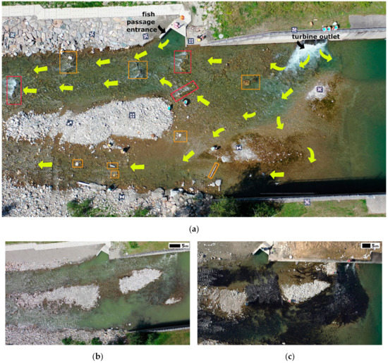
Figure 1.
The study area: (a) at the time of the described experiment, in August 2019 (yellow arrows indicate visually identified flow directions, red rectangles show locations of river thresholds; orange rectangles contain areas where flow is obstructed by obstacles); (b) in June 2019; (c) in February 2019.
Within the region of interest, the river is not particularly deep, between 0.1 and 2.0 m. The colour of water in the river has variations, changing from transparent (Figure 1a,c) to turbid green (Figure 1b). The riverbed is rocky, almost black in winter (Figure 1c) and brown-green in the summer months (Figure 1a). Water level is characterised by fluctuations, and parts of the riverbed may be exposed to the air depending on the season. In the middle of the river there are islands made up by boulders and cobbles. The locations and shapes of the islands change to some extent after each flood as well as depending on the water level (compare Figure 1a–c). The test site is characterised by heterogeneous flow with partially opposite flow directions (Figure 1a) and velocities ranging between zero and approximately 2 m/s.
To acquire reference flow velocities, we used a propeller current meter OTT C31 and performed measurements in 23 locations directly under the water surface (Figure 2). These locations were selected in a way that enabled assessment of performance of non-intrusive measurements for all the important components of the flow in the FOV. These components included the main flow from the turbine outlet, areas around the main flow curve, two branches of the main flow after its split, and the flow from the fish entrance. To perform velocity measurements, the current meter was placed in water in such a way that propeller axis aligned with the direction of the flow. The duration of measurement at each point was one minute. Flow directions were determined with 10° precision with the help of a compass. Differential GPS with a 2–3 cm positioning accuracy was used to determine the coordinates of the reference flow measurements.
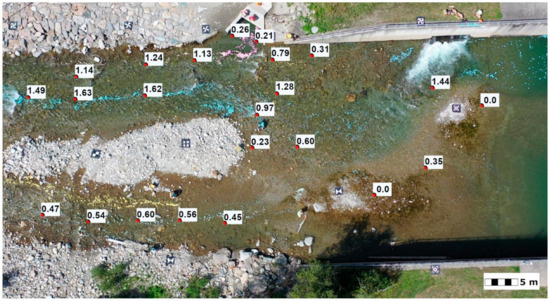
Figure 2.
Locations of reference measurements with flow velocity magnitudes in m/s.
Data acquisition (Please find in Supplementary) was performed with the use of a DJI Mavic Pro drone. This lightweight (0.8 kg) quadcopter has a horizontal positioning accuracy of ±30 cm + 1 ppm and a vertical positioning accuracy ±10 cm. Its built-in camera has the following parameters: 1/2.3”, 26 mm F/2.2, 78.8°, equivalent to 35 mm, distortion 1.5%. Maximum video resolution for this camera is 3840 x 2160 px at 24, 25 or 30 fps. In addition to its relatively low cost (approximately EUR 1000), another advantage of this UAS is an automatic correction of the barrel distortion. The video was captured in a hovering mode at 25 fps from the altitude of 50 m.
Eleven ground control points (GCPs) were present in the field of view (FOV) in the captured video. The GCP markers were produced from white plastic with black printed patterns. The marker dimensions were 80 x 80 cm. In order to increase the contrast between the markers and the background, pieces of black pond liner approximately 130 x 130 cm in size were placed under each of the GCP markers. The locations of the GCP markers were determined with the use of the differential GPS with a 2–3 cm positioning accuracy.
For seeding of the flow, we used ecofoam of different colours (azure, pink, yellow and light green). The choice of tracer was motivated by the fact that ecofoam has proved to be a good seeding material for LSPIV analysis [40,54,55]. The tracers were introduced into the flow from seven different locations: from over the turbine outlet, from over the entrance into the fishway, from one of the islands in the direction of the dominant flow, from two other islands and from the two banks. The ecofoam was purchased from the seller of ecological packaging materials Biobiene. These tracers are made out of corn and coloured with environmentally friendly dyes, are buoyant and biodegradable. Individual ecofoam pieces have cylindrical shape, 1.5–2 cm in diameter and 4.5–6 cm in length. Once in water, the pieces tend to stick together, forming clusters of different size and shape that are easy to recognise in a video recorded from a 50 m altitude.
The video recording started about 40 seconds before the introduction of tracers into the flow. A signal horn was used in order to indicate the start of the seeding. Starting with the second minute of the recorded video, most of the areas of interest had some tracers present. The best seeding of the area near the entrance into the fish ladder was achieved in about three and half minutes from the start of the video recording and was present for about 30 seconds. The complete video duration was five minutes, with approximately two minutes of the video file featuring relatively dense seeding in the areas of interest within the FOV.
As mentioned above, we used PIVlab [45] to perform data evaluation. PIVlab is a popular MATLAB-based software that has proven its quality in many previous studies [20,22,26,36,56,57,58,59,60,61]. It is Open Source and can be used for free, and it is actively developed and well supported. PIVlab offers a series of image pre-processing options and post-processing techniques. Another advantage of this software is its intuitive GUI. The newest version of the software (v.2.31, released October 2019) features ensemble correlation and can automatically calculate recommended PIV settings for the selected region of interest. PIV can process bmp, jpeg/jpg and tiff/tif image files. Image extraction from video files and image stabilisation do not belong to the PIVlab functionality.
To extract images from the video file, we used a custom MATLAB script. We sub-sampled the frames, extracting each second frame, thus creating an image sequence with a time interval of 80 ms between the consequent frames. This frame rate was a compromise that allowed simultaneous PIV application to different areas of the heterogeneous flow in the FOV. The original frame rate of 25 fps was too high to analyse the areas with low flow, while further increase of time interval between analysed frames reduced the quality of correlation in the areas with high flow velocities. Image calibration resulted in a ground sampling distance (GSD) of 0.021 m/px.
The selected image sequence had to be stabilised before PIV application. Due to the camera movement, images in the sequence experienced a vertical shift of approximately 13 px and a slight (1.6°) clockwise rotation. We performed image stabilisation with the use of MATLAB and some of the built-in methods of PIVlab, applying a six-step algorithm:
- Visual identification of motionless features that can be tracked, e.g. GCP markers that are present in all the frames across the analysed sequence.
- Identification of coordinates of these motionless features (in pixels) in the reference image.
- Optional: Image enhancement in order to increase the contrast between the tracked features and the background.
- Calculation of the displacements of the motionless features with regards to a reference image with the help of multipass the FFT with the 2 × 3-point Gauss sub-pixel estimator (a PIVlab method).
- Calculation of the new coordinates of the tracked features based on determined displacements.
- Affine image transformation with the help of two sets of coordinates of the tracked features: in the reference image and in the currently analysed frame.
The root mean square error (RMSE) of stabilisation for any two consecutive frames was on average 0.17 px. Thus, velocities calculated by means of PIV from these frames were a subject to a stabilisation error of 0.045 m/s on average.
Out of the stabilised frame sequence, we selected 121 consecutive images with the goal to perform a series of analyses varying the PIV settings. The images featured relatively dense but inhomogeneous seeding near the fishway. Seeding of this area was particularly important, since a wave pattern near the fishway complicated the non-intrusive calculation of the correct flow pattern. Figure 3 illustrates the flow pattern derived by means of PIV based solely on wave pattern, with no seeding. It shows no flow out of the fishway, which is known to be wrong. The actual flow pattern, featuring a flow out of the fishway entrance, was revealed when tracers were added into the water, which is demonstrated in the Results section of this paper.
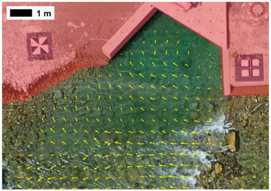
Figure 3.
Wave pattern near the fishway.
After selecting the frames, we cropped them to the area in the close proximity of the fishway, with the dimensions of 1800 × 1000 px, which corresponded to approximately 38 × 21 m2. The decision to crop the images was motivated by the necessity to reduce the computational cost of the comparison of velocities associated with different PIV settings. The area selected for the comparative analysis provided a good representation of overall flow conditions in the FOV due to the complex flow structure. It featured a confluence and two swirls. Moreover, the flow was obstructed in some locations, creating turbulent spots and areas that were difficult to seed. The reference velocities near the fishway measured at seven locations where at least some tracers were present, ranged from 0.21 m/s to 1.62 m/s.
Viewing the cropped frames as a sequence of 120 image pairs, we performed velocimetry with eight sets of PIV settings given in Table 1. Across all sets of settings, we used the spline deformation of the IA, 5 × repeated correlation and 2 × 3-point Gauss sub-pixel estimator.

Table 1.
Particle image velocimetry (PIV) settings for comparative analysis of the cropped image sequence.
The PIV settings resulting in velocities that were in the most agreement with the magnitudes of reference velocities were used further to analyse the second image sequence. The second sequence included 230 images (120 of which belonged to the first image set) which were used as 115 image pairs. The seeding density and homogeneity in different areas of the ROI varied across the second image sequence. Regions, which were poorly seeded in some of the frames, were well seeded in others. For example, the density of seeding near the fishway varied between 6.8 × 10⁻⁴ and 3.3 × 10⁻³ particles per pixel (ppp). The seeding density of the dominant flow was between 1.2 × 10⁻³ and 9.2 × 10⁻³ ppp. The flow from the fish passage along the bank was seeded with the density of 1.1 × 10⁻³ to 3.1 × 10⁻³ ppp. Sizes of identifiable particles varied depending on the flow conditions, too: in the areas of low flow, ecofoam often built large clusters containing dozens of particles, while in areas where flow velocities were high, individual particles or small clusters could be observed. In swirls, tracers accumulated over time.
Image pre-processing within our workflow included an automatic contrast stretch and the application of a high-pass filter with 60 px Kernel size. Both of these pre-processing procedures were carried out with the use of the standard functionality of PIVlab. An example of image pre-processing results juxtaposed to a portion of an original image is given by Figure 4.
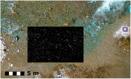
Figure 4.
An example of image pre-processing results juxtaposed to a portion of an original image.
Image post-processing was performed with the use of the standard PIVlab tools. Erroneous vectors were removed with the use of the standard deviation filter with a threshold of seven standard deviations, and applying the local median filter with default settings. Other methods of data post-processing such as manual vector removal or imposing limits on flow velocity were not applied. The results of the PIV analysis of the second frame sequence were compared with the complete set of reference measurements, in terms of both velocity magnitudes and flow directions.
3. Results
3.1. Comprison of Velocimetry Results Associated with Different PIV Settings
To compare reference velocities with the PIVlab values, we used the following approach:
- Reference measurements were converted into relative coordinates in metre, such that point (0; 0) corresponded to the top left corner of the FOV. Image coordinates of GCP markers used for transformation were identified manually in a free image editor GIMP.
- Continuous velocity and direction fields produced by means of PIVlab were exported into tab-separated text files. The resolution of the acquired dense velocity field (split in two files, magnitude and direction) corresponded to GSD.
- Then, we identified the cells in the exported dense velocity field, which corresponded to the locations of reference measurements: indexes of corresponding rows and columns were calculated by dividing relative coordinates of reference measurements by GSD.
- The PIV value for each of the reference measurements was calculated as a median of nine cell values, the cell identified in the previous step and eight surrounding cells, since accuracy of reference data coordinates was 2–3 cm, plus and uncertainty of approximately 1 cm was associated with coordinate transformation.
- Information on the reference measurements and corresponding PIV values associated with each set of the analysis settings are provided in Table 2. Relative differences (in %) between the PIV velocities and the reference values, and their statistics are given in Table 3.
Table 2. Reference measurements and PIV velocities for eight sets of analysis settings.
Table 3. Relative differences (in %) between the calculated PIV velocities and the reference measurements. Statistics are grouped by (a) the interrogation area (IA) size and the correlation method (b) the correlation method only.
As initially expected, PIV settings that relied on the standard FFT correlation and subsequent velocity averaging (S1–S4) resulted in SVFs that systematically underestimated the flow velocities. The calculated values were lower in comparison to the reference values by 0.11 m/s and 19.7% on average, with median difference values of −0.10 m/s and −9.7%. In about 2/3 of the cases, PIV based on the ensemble correlation (settings E1–E4) also underestimated flow velocities. However, for the settings associated with the ensemble correlation, mean differences between the reference measurements and the calculated values were 0.07 m/s and 9.4%, whereas median differences equalled to −0.05 m/s and −5.1%.
Figure 5 displays the spatial distribution of reference measurements near the fishway. Surface velocity fields calculated for each set of PIV settings are visualised in Figure A1. The reference velocity 0.21 m/s is located very close to the fishway entrance near the right wall. In order to increase the flow velocity near the opposite wall, the flow near the right wall is artificially obstructed, and a circular flow pattern is formed. None of the PIV settings based on the standard FFT correlation (S1–S4) led to an accurate calculation of the flow velocity in this area, underestimating the actual value by 0.14–0.17 m/s. Ensemble correlation (settings E1–E4), however, yielded results that were within a difference of 0.01–0.07 m/s from the reference measurement.
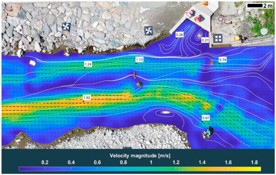
Figure 5.
Spatial distribution of reference measurements near the fishway and a surface velocity field (SVF) calculated by means of PIV with settings S4.
PIV velocities at the location of the reference value 0.26 m/s (measured at the fishway entrance) were characterised by high accuracy, within 0.01–0.04 m/s across all eight sets of analysis settings. Settings E1–E4 overestimated this value by 0.01–0.04 m/s, while settings S1–S4 underestimated it by 0.01–0.03 m/s. The same trend was observed near the reference value 0.97 m/s, where settings based on ensemble correlation overestimated the velocity by 0.04–0.11 m/s, while the standard correlation approach led to values underestimated by 0.09–0.17 m/s.
For the reference value 1.62 m/s, the associated PIV velocities had an accuracy of 0–0.06 m/s with no significant differences between the settings. PIV velocities downstream from the fishway entrance near the riverbank were determined with lower accuracy across all analyses. The values calculated with analysis settings E1–E4 were 0.10–0.15 m/s lower that the reference velocity of 1.13 m/s; settings S1–S4 underestimated this value by 0.17–0.31 m/s. Calculated low values are unlikely to be associated with insufficient seeding since the reference measurement was done in one of the best seeded areas of the ROI. Velocities at other reference locations were underestimated within 0.06–0.12 m/s depending on analysis settings. It is remarkable, that PIV velocities determined with the highest accuracy across all analysis settings, 0.26 m/s and 1.62 m/s, are the velocities of the flow from the fishway and the velocity of the dominant flow, respectively.
The calculated flow pattern (Figure 5) contained all the elements known to be present in the ROI. Two circular flow structures, near the fishway entrance and near the island, were correctly identified. Dominant flow was located correctly, too. As expected, the flow near the riverbank was characterised by lower velocities than the dominant flow. Places where the flow was obstructed could be identified from the SVF as well: the flow velocity at obstacles visibly dropped and flow direction changed. An apparent unexpected drop in flow velocity in some areas was associated with the presence of river thresholds. Here the application of PIV was challenging due to both the high turbulence influencing the visibility of tracers and the vertical direction of tracer movement.
Independent of the applied analysis settings, all SVFs contained two areas of apparent low flow velocities that did not necessarily describe the flow with the due level of accuracy. One such area was behind an obstacle, downstream from the reference measurement of 1.13 m/s, and another one was in the centre-right part of the image. Since they were poorly seeded, no visually identifiable movement could be observed within these areas in the majority of analysed images, likely leading to underestimated velocity values. An application of settings E1–E4 yielded slightly higher flow velocities in the area downstream from the obstacle than the use of settings S1-S4 (Figure A1: compare images in the left column [S1–S4] with the images in the right column [E1–E4]).
Special attention should be paid to streamlines near the entrance into the fish passage. Though some of the processed frames contain information about the seeding particles moving along the left wall and continuing their way in the downstream direction along the riverbank, none of the flow patterns derived with eight sets of PIV settings yielded an SVF that would depict such flow pattern. On the contrary, the streamlines at the fishway entrance in most SFVs were pointed away from the actual flow direction. This is due to the fact that the wave pattern discussed above interfered with the calculation of velocity vectors near the fish ladder. To avoid this interference, a larger size of IA should be used for PIV analysis. Figure 6 shows an example of SVF calculated with a two-pass standard correlation FFT with IA sizes of 96/96 px and 96/48 px.
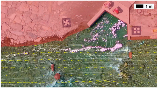
Figure 6.
A flow pattern near the fishway calculated with the use of large IA: 96/96 px in the first pass and 96/48 px in the second pass.
The streamlines in the Figure 6 correctly represent the flow in the area influenced by the wave pattern in previous analyses. However, the used IA size is too large to determine the circular flow pattern near the right fishway wall, and the overall spatial resolution of the SVF is too low. Thus, it is suitable for the first, high-level analysis of the flow structure but cannot be considered sufficient for the task in hand. Among the more detailed SVFs calculated with the use of settings S1–S4 and E1–E4, the patterns described by images Figure A1a–c,e,g in Appendix A characterise the flow more realistically. They reflect the fact that most of the tracers in the recorded image sequence first moved into the direction of the right wall and only then joined the main flow.
After comparing the results of application of different PIV settings, we selected a set of settings for the analysis of the second frame sequence. Considering the fact that a number of reference measurements within the FOV of the first image sequence was small, we decided to base our choice on several factors rather than on a single statistic. We proceeded in the following way:
- Since settings based on the ensemble correlation in many cases led to more accurate PIV results, we decided to limit our choice to one of the settings from the group E1–E4.
- Among the settings E1–E4 we selected those where the statistics of differences between the PIV values and the reference values were the lowest, namely E1 and E4.
- Finally, we selected settings E4 for the final analysis since they underestimated PIV values less often. In addition, both the RMSE and the mean magnitude of differences (without consideration of sign) were lower for E4 than for E1. Another reason for analysing the large image sequence with settings E4 was the less typical size of the IA than the one used in E1. Since the majority of studies employ interrogation areas of 64/32/16 px, we considered it useful to demonstrate that PIV analysis may be performed with alternative IA sizes. Though initially the application of FFT required that IA had dimensions making the power of two (8, 16, 32, 64, 128, etc.), these days it is not the case [62], and therefore one can be more flexible in using other IA sizes when necessary.
3.2. Full-Scale Analysis of Flow Patterns
230 full-scale images (3840 × 2160 px) were analysed with the help of two-pass PIV based on ensemble correlation; the IA sizes were 48/48 px in the first pass and 48/24 px in the second pass. In the resulting SVF (Figure 7), the distance between vectors corresponded to approximately 50 cm.
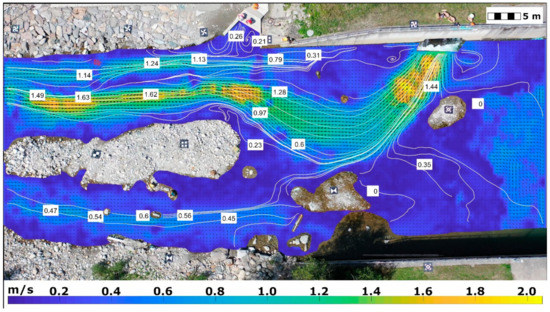
Figure 7.
SVF calculated with the help of PIV with ensemble correlation, first pass IA 48/48 px, second pass IA 48/24 px. Maximum velocity value is located in a turbulent sub-region near the turbine outlet and constitutes 2.06 m/s.
PIV has correctly determined the important elements of the flow structure: the dominant flow, the flow from the fishway entrance, and circular flow patterns near the fishway, near the turbine outlet and in the vicinity of the larger island. Changes in flow direction and velocity caused by obstacles were clearly indicated. The connection between the flow from the fishway entrance and the main flow was clearly indicated as well. It is represented through a streamline that averages two observed tracer trajectories: along the left wall directly into the main flow and, alternatively, towards the vortex near the right wall, and then into the main flow. To the right from the turbine outlet, below the nearby vortex, almost no tracers could be observed in the video recording. The velocity vectors calculated in this area are based exclusively on the wave pattern and are not necessarily accurate. The area in the right bottom part of the ROI experienced poor illumination and therefore was masked out for the PIV analysis. This resulted in an interrupted streamline below the island where a GCP marker with an hourglass pattern was placed.
Table 4 (columns A–D) juxtaposes the calculated velocity magnitudes and the reference measurements. In the majority of cases, PIV slightly underestimates the reference velocities; however, in some of the areas (e.g. in the bottom part of the main flow right after the split), the velocity values appear to be slightly overestimated.
Table 4.
PIV results for the entire ROI compared to the reference measurements and statistics of differences. Values in parenthesis in column B are PIV results from the analysis of the first image sequence. Differences in flow direction are given as magnitudes (unsigned) since angles are circular data.
Flow velocity at the location of the reference value 0.35 m/s is the only one strongly underestimated (the calculated value is 0.08 m/s, −77.1% difference), which can be explained by the fact that almost no visible tracer movement could be observed in this area. Flow velocity in the vortex near the fishway entrance (reference value 0.21 m/s) appears to be underestimated, too, though less considerably (the measured value is 0.14 m/s, −33.3% difference, compared to 0.22 m/s in the previous analysis with settings E4). At the same time at the location to the left from the vortex, where reference velocity has the magnitude of 0.26 m/s, the current PIV result is 0.27 m/s (the same as in the previous analysis with settings E4). The mean absolute difference between the calculated and the measured values is 0.07 m/s, the RMSE is 0.10 m/s, and the median lies by −0.04 m/s. The mean relative difference between the reference velocities and the PIV values is 11.8% (RMSE 20.2%). This value is strongly influenced by a large difference of −77.1% observed in the poorly seeded area near one of the islands. For seeded regions (excluding the one where the reference velocity 0.35 m/s was acquired), the mean relative difference between the reference values and the PIV velocities is 8.5% (RMSE 11.5%). RMSE of absolute differences between reference velocities and PIV values in seeded areas is 0.09 m/s.
The use of an extended frame sequence (Table 4, column B) has slightly decreased PIV performance near the fish passage. A large difference from previous PIV values (0.07 m/s and 0.10 m/s) was observed twice; in other cases, the calculated velocities remained nearly the same. 86% (18 out of 23) reference velocities were estimated to be within 15% of the measured values, 66% (14 out of 21)—within 10% and over 40% (9 out of 21) – within 5%. Though these are promising results, one has to keep in mind that a small number of reference measurements was available for comparison, and that the flow was reasonably well seeded. In unseeded areas, errors associated with PIV values are expected to be much higher, as becomes evident in the location where the reference velocity of 0.35 m/s was acquired.
Table 4 contains raw velocity values measured by means of a propeller current meter and calculated with the help of PIV. Comparison of raw velocity values, though common in the literature, is a simplified analysis method. Both flow measurement methods that are being compared deliver results within a certain uncertainty interval. For PIV, this uncertainty may be associated with the magnitude of the stabilisation error, with possible errors due to image noise, or errors resulting from the use of not optimal IA sizes. Some of these uncertainties, e.g., the uncertainty introduced by the image noise, are difficult to estimate in field conditions; for others, quantitative assessment can be performed. In this study, the stabilisation error introduces an uncertainty of 0.045 m/s on average. The accuracy of a propeller current meter lies within 2% of the measured value, which corresponds to 0.01–0.03 m/s for the range of velocity magnitudes in the study area. Figure 8 provides a visual representation of velocity magnitude comparison, including the consideration of uncertainties associated with current meter accuracy and image stabilisation. In 47% of cases, the uncertainty intervals associated with the reference measurements and the PIV velocity magnitudes completely or partially overlap. In cases of non-overlapping uncertainty intervals, the difference between them constitutes 0.06 m/s on average.
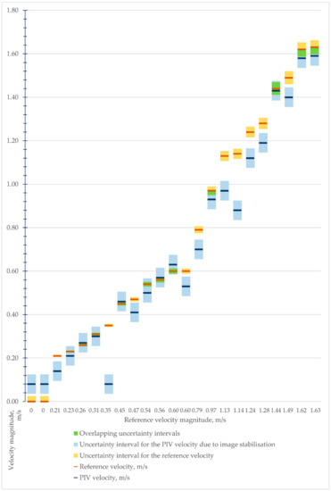
Figure 8.
Comparison of measured and calculated flow velocity magnitudes.
The last step of the analysis was the comparison of reference flow directions with flow directions determined with the help of PIV (Table 4, columns E–G). Since in PIVlab 0° corresponds to East of the image, and possible angle values range from −180° to 180°, the extracted PIV angle values were first unified with the reference directions by adding 360° to negative angle values and then aligning the 0° with North. Figure 9 provides a visual representation of comparison of measured and calculated flow directions. To the best of our knowledge, there exists no standard approach to estimation of direction uncertainty associated with image stabilisation when dealing with LSPIV. In Figure 9, the uncertainty associated with the 10° precision of reference measurements is depicted as an interval surrounding reference velocities. A direction uncertainty associated with image stabilisation could not be calculated for each of the reference measurements based on average stabilisation error or main direction of camera movement, and therefore it was not analysed. Figure 9 shows that the majority of the directions determined by PIV are consistent with reference measurements, with an average difference between the reference angle and the measured angle constituting 22° (12.2% of maximum possible difference of 180°) and a median difference of 13° (7.2%).
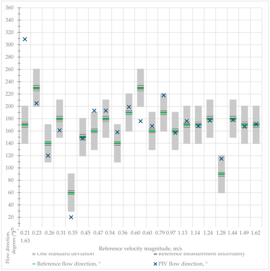
Figure 9.
Comparison of measured and calculated flow directions. Markers that represent the measured angle of the flow direction (green horizontal lines) are surrounded with an uncertainty interval associated with the precision of reference measurements (a striped pattern). Grey areas that visualise a range of ±31°, which corresponds to 1 standard deviation, are added in order to simplify the visual assessment of PIV performance.
The largest difference between the measured and the calculated flow direction across all reference measurements was associated with the velocity of 0.21 m/s. A possible reason is that this velocity was measured inside a vortex. Thus, it is not excluded, that the reference direction of the flow was determined incorrectly.
In the majority of cases, flow direction is more accurately identified for higher flow velocities. This can be explained by the fact that low flow velocities are associated with small particle displacement between frames, which makes angle calculation more difficult. For flow velocities that exceed 1 m/s (which roughly corresponds to a particle displacement of 4 px/frame), the unsigned difference between reference flow directions and PIV flow directions was less than 10° for all but one measurements. The only larger difference (25°) was associated with a value measured in a turbulent sub-region near the turbine outlet, where correct identification of flow direction is challenging regardless of the used measurement approach. In homogeneous low flow conditions, a higher accuracy of flow direction calculation with the help of PIV could be achieved by means of image sub-sampling and increasing the time interval between subsequent image frames.
Analysis results indicate that LSPIV can accurately determine the major elements of a heterogeneous flow pattern near a fish passage in seeded flow conditions. The largest error in PIV results in terms of velocity magnitude is observed in a poorly seeded area. The largest differences between a measured and a calculated flow direction is observed in a swirl where correct identification of flow direction may be challenging regardless of a measurement method used.
When dealing with sequences of a little over 100 image pairs, where seeding is present but not homogeneous, multipass ensemble correlation improves PIV results in comparison to the traditional FFT correlation approach. Varying interrogation area size affects not only the density of the resulting SVF, but also the accuracy of velocity assessment. Refinement of the IA size in each FFT pass does not always benefit the velocimetry results, e.g., keeping the IA size low and constant in the first pass may be advantageous for the areas with lower velocities. Flow directions determined with the help of LSPIV are in a good agreement with the reference directions. This is an important finding, considering the fact that identification of flow directions plays an important role when dealing with the analysis of flow conditions near fish passages.
4. Discussion
It is well known that the size of IA used for PIV analysis influences the ability of the algorithm to correctly determine flow velocities [34]. In this study, the velocities range from zero to approximately 2 m/s. Considering the GSD of 0.021 m/px, the observed displacement of tracer particles may be as high as 7.5–8 px/frame. Thus, if one-pass FFT correlation with no IA deformation is used, reliable velocimetry results may be yielded for the IA of at least 32 × 32 px. This IA size, corresponding to approximately 0.6 x 0.6 m in reality, is not necessarily optimal for capturing finer circular flow structures present in the FOV. The use of multipass FFT with IA size refinement allows accounting for both the necessity to accurately calculate high velocities, and the need to determine the presence and to measure the velocities in small and circular flow structures.
The comparison of eight sets of multipass PIV settings has shown that for low velocities it is advantageous to start with a smaller IA and keep it constant in the first pass, and then to refine it in the second pass. At the same time, since small IA size makes PIV more sensitive to small-scale flow variations, this choice of settings may obscure more general flow patterns. For instance, in the vicinity of the fishway entrance, small waves that move in the direction opposite to the flow distort the calculated flow pattern when small IA sizes are used. The distorted vector field shows no flow from the fishway joining the main flow (Figure A1c,d), even when the IA size before the first refinement is sufficiently large to capture a more general pattern (Figure A1f).
Since IA size has a significant influence on PIV results, it is advisable to preliminary analyse the flow with a reasonably large IA and a two-pass FFT with no IA refinement in the first pass. Such an analysis is likely to result in underestimated velocity values, but it can provide a good understanding of high-level flow structure and main flow directions, and its computational cost is little. Image enhancement for this preliminary analysis may be done in a way different from the main analysis, e.g., denoise filters can be set to higher values, because small-scale local flow variations at this stage can be ignored. The preliminary analysis may be helpful for later SVF validation: the refinement of the IA should add more detail and increase spatial resolution of the SVF, but should not completely inverse flow directions (unless within circular structures).
The performance of PIV in this study is consistent with the previous studies that exploited LSPIV for flow analysis [24]. Previous research has shown that LSPIV based on standard FFT correlation or DCC is prone to underestimating flow velocities due to insufficient seeding density [48,49,63,64]. Our results have also indicated that independent on the correlation method employed, LSPIV tends to underestimate flow velocities; however, the use of ensemble correlation that averages correlation matrices before determining the correlation peak, in many cases reduces the magnitude of differences between the reference velocities and the PIV values. The unsigned differences between the reference velocity magnitudes and PIV values constituted on average 0.11 m/s (19.7%) for a standard multipass FFT correlation method and 0.07 m/s (9.4%) for ensemble correlation, with RMSE of 0.13 m/s (31.0%) and 0.08 m/s (11.3%), respectively.
Our tests included sequences of 115 and 120 image pairs where seeding of the flow was not homogeneous: in some frames, the main flow was well seeded, but the flow from the fishway was seeded insufficiently; other frames where characterised by the opposite trend. In these conditions, ensemble correlation had an advantage over the standard FFT correlation approach. The mean absolute difference in velocity magnitude between the PIV values and the reference measurements was 0.07 m/s for both frame sequences, with RMSE of 0.08 m/s for the first frame sequence (across settings E1–E4) and 0.10 m/s for the second frame sequence.
It is important to stress, that ensemble correlation is usually used with short image sequences. A significant increase in the number of processed image pairs will increase the computational costs of data processing and may negatively influence correlation results. Therefore, the frames used for analysis have to be selected carefully. Seeding in the areas of interest may be inhomogeneous, but each area of interest should be seeded with tracers at least in some of the analysed frames.
Our results indicate that changing the correlation approach in the areas with no seeding had little influence on PIV results. A PIV velocity that was calculated with ensemble correlation for an unseeded area with no visible movement was largely underestimated (reference value 0.35 m/s vs. PIV value 0.08 m/s, 77.1% difference). In the seeded areas, the difference between PIV velocities and reference values rarely exceeded 15%. Since no natural tracers were present in the flow, in unseeded areas flow patterns could only be calculated from the wave patterns. However, the very idea of deriving flow patterns based solely on wave patterns should be viewed critically, especially in low flow conditions and in cases of heterogeneous flow. For instance, in our study, certain areas within the FOV were characterised by a wave pattern dissimilar from the flow pattern. In the centre-right part of the FOV, a wave pattern could indicate flow velocities of up to 0.80 m/s. During the experiment, we did not target this area with seeding since it was of less interest considering the task in hand. However, some of the tracers could be found here, and they experienced no apparent movement. Thus, the observed wave pattern and the pattern of tracer displacement clearly contradicted each other. A similar situation was observed directly near the fishway entrance, as was discussed above. Therefore, in flow conditions similar to ones presented in this study, successful application of LSPIV cannot be ensured for unseeded flow. To avoid the effect of misleading standing waves that are known to negatively influence PIV results [24], in the absence of natural seeding, artificial eco-friendly tracers should be used.
The performance of PIV varied in different areas of the observed heterogeneous flow. For example, flow directions determined by means of PIV were subject to a greater error in the areas of low flow than in the areas where flow velocities were higher. The accuracy of calculation of flow directions in the areas of low flow can be improved by increasing the time interval between the analysed video frames (e.g., reducing the frame rate to 5 fps). In heterogeneous flow conditions, as presented in the current study, this will simultaneously reduce the performance of PIV in areas of higher velocities. Ideally, an optimal frame rate should be selected individually for different sub-regions of heterogeneous flow based on individual flow characteristics in each sub-region. Unfortunately, processing image sequence with variable time intervals between the frames and adjusting PIV settings to the characteristics of individual sub-regions within the FOV is not yet supported by PIVlab or other comparable software.
The analysis of the second image sequence has shown that PIV underestimated the velocities associated with the flow from the fish passage to a greater extent than the velocities in other seeded sub-regions of the FOV. However, underestimating flow velocities in this area is less critical than overestimating them: it means that, in fact, fish have higher probability of discovering an entrance into the fish passage than estimated. At the current stage of method development, considering the main goal of the research, the performance of PIV can be considered acceptable: it correctly determines the major elements of the flow in the FOV, and identifies differences between sub-regions of the FOV. The results of PIV analysis unambiguously state, which of the FOV sub-regions are characterised by the highest and the lowest velocities. They show that after the split the velocity of the main flow near the fishway is higher than the velocity of the flow from the fishway entrance, and that the second branch of the main flow is characterised by lower velocities than those from the fishway entrance. For the task in hand, the ability to quickly acquire this information is of great value. Further development of the non-intrusive flow analysis approach will address the improvement of measurement accuracy. Possible directions of improvement may include optimisation of flow seeding and local adjustments of PIV settings. In general, the development of an analysis approach that supports variable frame rates and PIV settings for sub-regions of the FOV will be beneficial for PIV performance in heterogeneous flow conditions that are observed near fish passages.
The use of a drone for video data acquisition provides a lot of flexibility in selecting an area for an optical analysis of the flow. The wider the river, the more uncertainty is introduced to a video recording from the riverbank due to an increasing degree of perspective distortion. Though this angle of video recording may be still suitable for estimating the average flow velocity or discharge [41,53,65,66], it does not allow to recognise small-scale flow patterns, especially in the areas that are closer to the riverbank opposite to the one where the camera is mounted. The use of cameras mounted on and under bridges limits data acquisition to areas where bridges are present. UAS as a camera-carrying platform has no such limitations. This proves to be very useful, for example, when dealing with flood events [27]. Helicopters have also been successfully used for aerial data capture during floods [42], but the cost of their use is substantially higher than the cost of a drone-based data collection. Therefore, in the scientific community there is a clear trend of shifting towards drone-based video data acquisition for optical flow measurements (compare [39,42] to [25], [57] to [20], [67] to [48]).
With flexibility to collect data in a wide variety of areas, a successful application of LSPIV is limited by the necessity of flow seeding. Though natural tracers can be present in water in abundance, this is not always the case. During flood events, artificial seeding of the flow is mostly unnecessary [66]. Wave crests can sometimes be used as features to track [57]. In less extreme flow conditions, wave patterns may not be representative as our study and other studies [40] have shown, and other traceable features may be absent. Thus, the choice of area for data acquisition for further processing with LSPIV has to take into account the possibility of artificial flow seeding. In most experiments that included an artificial seeding of the flow, tracers were introduced from the bridge over the river [20,60,68], and river width rarely exceeded 20 m. When using LSPIV to determine flow patterns near fish passages at hydropower dams, one deals with the necessity to seed a large area (river width 35 m and more). Introducing tracers from the dam is unreasonable since most of them will be captured in the areas near the dam where water is steady. In this study, there were islands present in the middle of the river, which simplified the seeding of the area of interest. On many other sites near fish passages, it is only possible to use riverbanks as seeding positions, making it hard to ensure that river middle is sufficiently seeded. Further research is necessary for the development of an efficient seeding workflow in such conditions.
One current limitation of LSPIV flow measurements near fish passages is the maximum resolution of affordable video cameras, most of which can record videos of no more than 4096 × 2160 px. The development of technology is likely to naturally overcome this limitation in the following years. Current solutions of this problem include the use of drone swarms and image stitching, or reducing the level of detail in the entirety of ROI while also recording a video at lower altitude in the direct proximity of the fishway.
Since PIV is sensitive to the IA size, further research may address an issue of ROI segmentation and automatic adjustment of PIV settings to velocity ranges that characterise different ROI segments. The first step in this direction has already been done, with the new functionality of PIVlab offering automatic calculation of PIV settings for a selected region. Varying PIV settings depending on differences in ROI segments may increase PIV accuracy in heterogeneous flow conditions, such as near fish passages at hydropower dams.
5. Conclusions
River sections near fish passages at hydropower dams are characterised by heterogeneous flow conditions, including varying and sometimes opposite flow directions, presence of circular flow structure and wide velocity ranges. Being a part of research devoted to the increase in fish passage efficiency, this study explored a possibility of application of LSPIV for flow pattern analysis near fish passages. Within the region of interest, the river was up to 35 m wide, with small islands in the middle. Turbine outlet and fishway entrance were present in the field of view.
Flow data was collected with a low-cost UAS with a built-in 4K camera. Pointwise reference measurements were made with the help of a propeller current meter, and flow directions were identified with the help of a compass with 10° accuracy. MATLAB based software PIVlab was used for PIV analysis.
First, we analysed a sequence of 120 image pairs cropped to the area in the close proximity of the fishway entrance using eight sets of PIV settings. A high pass filter with 60 px Kernel size was applied for image enhancement. The analyses showed that, probably due to inhomogeneous seeding, PIV with standard FFT correlation approach systematically underestimated flow velocities by 0.11 m/s and 19.7% on average. PIV based on the ensemble correlation, on the other hand, improved the analysis accuracy and yielded results that were in a better agreement with reference values (mean absolute difference 0.07 m/s, mean relative difference 9.4%).
The second sequence of 115 inhomogeneously seeded frame pairs depicting the entire region of interest was analysed with a two-pass PIV based on the ensemble correlation. The selection of frames was done in a way that some seeding was present in each area of interest at least in some of the frames. Interrogation area of 48 × 48 px was kept constant in the first pass and refined to 24 × 24 px in the second pass. Analysis results show that multipass LSPIV based on the ensemble correlation can be successfully applied to short frame sequences in order to calculate flow patterns near fish passages. Though it still tends to slightly underestimate flow velocities (mean unsigned difference of 11.8% for the whole FOV and 8.5% for the seeded areas), it correctly determines the major elements of the flow, and unambiguously identifies differences between sub-regions of the FOV. In seeded conditions, even if the tracers are not homogeneously distributed, velocity magnitudes and directions derived with LSPIV based on the ensemble correlation are in good agreement with reference measurements, with an absolute difference of 0.07 m/s and 22° on average. In areas where no visible movement can be observed, LSPIV cannot be applied. However, all optical methods of flow analysis have this limitation.
Further studies are needed in order to test the approach discussed in this study on wider rivers where seeding of the flow is likely to be more challenging and deriving small-scale flow structures may require more effort. However, for the rivers as wide as 35 m, LSPIV is a promising method for flow pattern analysis near fish passages at hydropower dams. It has a potential to be used as a part of the flow monitoring methodology, facilitating, when possible, timely reaction to undesirable changes in flow conditions with the goal to increase fish passage efficiency.
Supplementary Materials
The dataset used in this study referred to Strelnikova et al. (2020): https://doi.org/10.4121/uuid:d75cb9e1-5a22-4946-bf51-4da658a789a3.
Author Contributions
All authors have read and agreed to the published version of the manuscript. Conceptualization, S.K., P.M., G.P., and H.M.; methodology, D.S., G.P., H.M., K.-H.A., P.M., R.S.; validation, D.S., G.P., S.K., H.M. and P.M.; formal analysis, D.S.; investigation, D.S., G.P., K.-H.A., S.K., P.M., U.S., and R.S.; resources, D.S., G.P., K.-H.A., S.K., P.M., U.S., R.S.; writing—original draft preparation, D.S.; writing—review and editing, G.P.; visualization, D.S.; supervision, S.K.; project administration, S.K., P.M., and G.P.
Funding
This research received no external funding. The publication of research results was financed by COST Action CA16219 “HARMONIOUS—Harmonization of UAS techniques for agricultural and natural ecosystems monitoring”.
Acknowledgments
The authors would like to thank the reviewers for valuable input that increased the quality of this paper.
Conflicts of Interest
The authors declare no conflict of interest.
Abbreviations
| DCC | Direct Cross-Correlation | PIV | Particle Image Velocimetry |
| FFT | Fast Fourier Transform | PTV | Particle Tracking Velocimetry |
| FT | Fourier Transform | RMSE | Root Mean Square Error |
| FOV | Field of View | ROI | Region of Interest |
| GSD | Ground Sampling Distance | SA | Search Area |
| IA | Interrogation Area | SVF | Surface Velocity Field |
| LSPIV | Large Scale Particle Image Velocimetry | UAS | Unmanned Aerial System |
Appendix A


Figure A1.
Visual comparison of velocities calculated with different PIV settings: (a) S1: Mean 64/32-32/16; (b) E1: Ensemble 64/32-32/16; (c) S2: Mean 32/32-32/16; (d) E2: Ensemble 32/32-32/16; (e) S3: Mean 96/48-48/24; (f) E3: Ensemble 96/48-48/24; (g) S4: Mean 48/48-48/24; (h) E4: Ensemble 48/48-48/24.
References
- Buadoin, J.-M.; Burgun, V.; Chanseau, M.; Larinier, M.; Ovidio, M.; Sremski, W.; Steinbach, P.; Voegtle, B. Assessing the Passage of Obstacles by Fish. Concepts, Design and Application; Onema: Paris, France, 2015. [Google Scholar]
- Larinier, M. Environmental issues, dams and fish migration. In Dams, Fish and Fisheries: Opportunities, Challenges and Conflict Resolution; Marmulla, G., Ed.; FAO: Rome, Italy, 2001; pp. 45–89. [Google Scholar]
- Directive 2000/60/EC of the European Parliament and of the Council of 23 October 2000 establishing a framework for Community action in the field of water policy (OJ L 327 22.12.2000 p. 1). Eur. Community Environ. Law 2010, 327, 879–969.
- Biermayr, P. Renewable Energy in Numbers 2018: Development in Austria based on 2017 data [in German]. December 2018. Available online: https://www.bmnt.gv.at/dam/jcr:939cb822-6f5f-41e3-bad4-6546feaf88e5/eEiZ2018-Brosch%C3%BCre.pdf (accessed on 19 January 2020).
- BMLFUW. Guideline to the construction of fish passages [in German]. Available online: https://www.bmnt.gv.at/dam/jcr:6069bf1d-68b9-4a5d-8825-a4e9dac64ee6/Leitfaden%20zum%20Bau%20von%20Fischaufstiegshilfen_19_12_2012_final.pdf (accessed on 19 January 2020).
- Larinier, M. Location of fishways. Bulletin Français de la Pêche et de la Pisciculture 2002, 39–53. [Google Scholar] [CrossRef]
- Piper, A.T.; Wright, R.M.; Kemp, P.S. The influence of attraction flow on upstream passage of European eel (Anguilla anguilla) at intertidal barriers. Ecol. Eng. 2012, 44, 329–336. [Google Scholar] [CrossRef]
- Larinier, M. Baffle fishways. Bulletin Français de la Pêche et de la Pisciculture 2002, 83–101. [Google Scholar] [CrossRef]
- Larinier, M.; Marmulla, G. Fish passes: types, principles and geographical distribution - an overview. In Proceedings of the Second International Symposium on the Management of Large Rivers for Fisheries, Sustaining Livelihoods and Biodiversity in the New Millennium, Phnom Penh, Cambodia, 11–14 February 2003; pp. 183–205. [Google Scholar]
- Nordlund, B. Anadromous Salmonid Passage Facility Design. Available online: https://www.westcoast.fisheries.noaa.gov/publications/hydropower/fish_passage_design_criteria.pdf (accessed on 19 January 2020).
- Larinier, M. Fishways - general considerations. Bulletin Français de la Pêche et de la Pisciculture 2002, 21–27. [Google Scholar] [CrossRef]
- Powers, P.D.; Orsborn, J.F. New Concepts in Fish Ladder Design: Analysis of Barriers to Upstream Fish Migration, Volume IV of IV, Investigation of the Physical and Biological Conditions Affecting Fish Passage Success at Culverts and Waterfalls, 1982-1984 Final Report; Bonneville Power Administration: Portland, OR, USA, August 1985.
- Williams, J.G.; Armstrong, G.; Katopodis, C.; Larinier, M.; Travade, F. Thiking like a fish: A key ingredient for development of effective fish passage facilities at river obstructions. River Res. Applic. 2012, 28, 407–417. [Google Scholar] [CrossRef]
- Wagner, R.L.; Makrakis, S.; Castro-Santos, T.; Makrakis, M.C.; Dias, J.H.P.; Belmont, R.F. Passage performance of long-distance upstream migrants at a large dam on the Paraná River and the compounding effects of entry and ascent. Neotropical Ichthyol. 2012, 10, 785–795. [Google Scholar] [CrossRef]
- DWA. Fact Sheet DWA-M 509. Fish Ladders and Fish Passable Structures - Design, Dimensioning, Quality Assurance; German Association for Water, Wastewater and Waste: Hennef, Germany, 2014. [Google Scholar]
- Gisen, D.C.; Weichert, R.B.; Nestler, J.M. Optimizing attraction flow for upstream fish passage at a hydropower dam employing 3D Detached-Eddy Simulation. Ecol. Eng. 2017, 100, 344–353. [Google Scholar] [CrossRef]
- Da Silva, L.G.M.; Nogueira, L.B.; Maia, B.P.; De Resende, L.B. Fish passage post-construction issues: analysis of distribution, attraction and passage efficiency metrics at the Baguari Dam fish ladder to approach the problem. Neotropical Ichthyol. 2012, 10, 751–762. [Google Scholar] [CrossRef]
- Tummers, J.S.; Winter, E.; Silva, S.; O’Brien, P.; Jang, M.-H.; Lucas, M.C. Evaluating the effectiveness of a Larinier super active baffle fish pass for European river lamprey Lampetra fluviatilis before and after modification with wall-mounted studded tiles. Ecol. Eng. 2016, 91, 183–194. [Google Scholar] [CrossRef]
- Goode, D. Particle velocity interpolation in block-centered finite difference groundwater flow models. Water Resour. Res. 1990, 26, 925–940. [Google Scholar] [CrossRef]
- Detert, M.; Johnson, E.D.; Weitbrecht, V. Proof-of-concept for low-cost and non-contact synoptic airborne river flow measurements. Int. J. Remote. Sens. 2017, 38, 2780–2807. [Google Scholar] [CrossRef]
- Hauet, A.; Morlot, T.; Daubagnan, L. Velocity profile and depth-averaged to surface velocity in natural streams: A review over alarge sample of rivers. E3S Web Conf. 2018, 40, 06015. [Google Scholar] [CrossRef]
- Bandini, F.; Bauer-Gottwein, P.; Garcia, M. Hydraulics and drones: observations of water level, bathymetry and water surface velocity from Unmanned Aerial Vehicles. Ph.D. Thesis, Department of Environmental Engineering, Technical University of Denmark, Lyngby, Denmark, December 2017. [Google Scholar]
- Sasso, S.F.D.; Pizarro, A.; Samela, C.; Mita, L.; Manfreda, S. Exploring the optimal experimental setup for surface flow velocity measurements using PTV. Environ. Monit. Assess. 2018, 190, 460. [Google Scholar] [CrossRef] [PubMed]
- Detert, M.; Weitbrecht, V. A low-cost airborne velocimetry system: proof of concept. J. Hydraul. Res. 2015, 53, 1–8. [Google Scholar] [CrossRef]
- Fujita, I.; Notoya, Y.; Shimono, M. Development of UAV-based river surface velocity measurements by STIV based on high-accurate image stabilization techniques. In Deltas of the future and what happens upstream: Proceedings of 36th IAHR World Congress: The Hague, The Netherlands, 28 June–3 July 2015; Mynett, A., Ed.; Curran Associates Inc.: Red Hook, NY, USA, 2016; pp. 6602–6611. [Google Scholar]
- Lewis, Q.W.; Rhoads, B.L. Lspiv measurements of two-dimensional flow structure in streams using small unmanned aerial systems: 1. accuracy assessment based on comparison with stationary camera platforms and in-stream velocity measurements. Water Resour. Res. 2018, 54, 8000–8018. [Google Scholar] [CrossRef]
- Perks, M.T.; Russell, A.J.; Large, A.R.G. Technical note: advances in flash flood monitoring using unmanned aerial vehicles (UAVs). Hydrol. Earth Syst. Sci. 2016, 20, 4005–4015. [Google Scholar] [CrossRef]
- Tauro, F.; Tosi, F.; Mattoccia, S.; Toth, E.; Piscopia, R.; Grimaldi, S. Optical tracking velocimetry (OTV): leveraging optical flow and trajectory-based filtering for surface streamflow observations. Remote Sens. 2018, 10, 2010. [Google Scholar] [CrossRef]
- Leitão, J.P.; Peña-Haro, S.; Lüthi, B.; Scheidegger, A.; De Vitry, M.M. Urban overland runoff velocity measurement with consumer-grade surveillance cameras and surface structure image velocimetry. J. Hydrol. 2018, 565, 791–804. [Google Scholar] [CrossRef]
- Fujita, I.; Watanabe, H.; Tsubaki, R. Development of a non-intrusive and efficient flow monitoring technique: The space-time image velocimetry (STIV). Int. J. River Basin Manag. 2007, 5, 105–114. [Google Scholar] [CrossRef]
- Nishino, K.; Kasagi, N.; Hirata, M. Three-dimensional particle tracking velocimetry based on automated digital image processing. J. Fluids Eng. 1989, 111, 384–391. [Google Scholar] [CrossRef]
- Lloyd, P.M.; Stansby, P.K.; Ball, D.J. Unsteady surface-velocity field measurement using particle tracking velocimetry. J. Hydraul. Res. 1995, 33, 519–534. [Google Scholar] [CrossRef]
- Brevis, W.; Niño, Y.; Jirka, G.H. Integrating cross-correlation and relaxation algorithms for particle tracking velocimetry. Exp. Fluids 2011, 50, 135–147. [Google Scholar] [CrossRef]
- Raffel, M.; Willert, C.E.; Scarano, F.; Kähler, C.J.; Wereley, S.T.; Kompenhans, J. Particle Image Velocimetry. A Practical Guide, 3rd ed.; Springer: Cham, Switzerland, 2018. [Google Scholar]
- Adrian, R.J. Twenty years of particle image velocimetry. Exp. Fluids 2005, 39, 159–169. [Google Scholar] [CrossRef]
- Tauro, F.; Petroselli, A.; Grimaldi, S. Optical sensing for stream flow observations: a review. J. Agricult. Engineer. 2017, 49, 199–206. [Google Scholar] [CrossRef]
- Cenedese, A. Eulerian and Lagrangian velocity measurements by means of image analysis. J. Vis. 1999, 2, 73–83. [Google Scholar] [CrossRef]
- Tauro, F.; Piscopia, R.; Grimaldi, S. PTV-Stream: A simplified particle tracking velocimetry framework for stream surface flow monitoring. Catena 2019, 172, 378–386. [Google Scholar] [CrossRef]
- Fujita, I.; Hino, T. Unseeded and seeded PIV measurements of river flows videotaped from a helicopter. J. Vis. 2003, 6, 245–252. [Google Scholar] [CrossRef]
- Dramais, G.; Le Coz, J.; Camenen, B.; Hauet, A. Advantages of a mobile LSPIV method for measuring flood discharges and improving stage–discharge curves. J. Hydro-Environ. Res. 2011, 5, 301–312. [Google Scholar] [CrossRef]
- Dermisis, D.C.; Papanicolaou, A.N. Determining the 2-D Surface Velocity Field around Hydraulic Structures with the Use of a Large Scale Particle Image Velocimetry (LSPIV) Technique. In Impacts of Global Climate Change, Proceedings of the 2005 World Water and Environmental Resources Congress, May 15-19, 2005, Anchorage, AK, USA; Walton, R., Ed.; American Society of Civil Engineers: Reston, VA, USA, 2005; pp. 1–12. [Google Scholar]
- Fujita, I.; Kunita, Y. Application of aerial LSPIV to the 2002 flood of the Yodo River using a helicopter mounted high density video camera. J. Hydro-Environ. Res. 2011, 5, 323–331. [Google Scholar] [CrossRef]
- Jin, T.; Liao, Q. Application of large scale PIV in river surface turbulence measurements and water depth estimation. Flow Meas. Instrum. 2019, 67, 142–152. [Google Scholar] [CrossRef]
- Huang, W.-C.; Young, C.-C.; Liu, W.-C. Application of an automated discharge imaging system and lspiv during typhoon events in taiwan. Water 2018, 10, 280. [Google Scholar] [CrossRef]
- Thielicke, W.; Stamhuis, E.J. PIVlab – towards user-friendly, affordable and accurate digital particle image velocimetry in MATLAB. J. Open Res. Softw. 2014, 2, 1202. [Google Scholar] [CrossRef]
- Westerweel, J.; Dabiri, D.; Gharib, M. The effect of a discrete window offset on the accuracy of cross-correlation analysis of digital PIV recordings. Exp. Fluids 1997, 23, 20–28. [Google Scholar] [CrossRef]
- Scarano, F.; Riethmuller, M.L. Iterative multigrid approach in PIV image processing with discrete window offset. Exp. Fluids 1999, 26, 513–523. [Google Scholar] [CrossRef]
- Tauro, F.; Petroselli, A.; Arcangeletti, E. Assessment of drone-based surface flow observations. Hydrol. Process. 2016, 30, 1114–1130. [Google Scholar] [CrossRef]
- Tauro, F.; Porfiri, M.; Grimaldi, S. Surface flow measurements from drones. J. Hydrol. 2016, 540, 240–245. [Google Scholar] [CrossRef]
- Santiago, J.G.; Wereley, S.T.; Meinhart, C.D.; Beebe, D.J.; Adrian, R.J. A particle image velocimetry system for microfluidics. Exp. Fluids 1998, 25, 316–319. [Google Scholar] [CrossRef]
- Westerweel, J.; Geelhoed, P.F.; Lindken, R. Single-pixel resolution ensemble correlation for micro-PIV applications. Exp. Fluids 2004, 37, 375–384. [Google Scholar] [CrossRef]
- Bradley, A.A.; Kruger, A.; Meselhe, E.A.; Muste, M.V.I. Flow measurement in streams using video imagery. Water Resour. Res. 2002, 38, 51-1–51-8. [Google Scholar] [CrossRef]
- Dobson, D.W.; Holland, K.T.; Calantoni, J. Fast, large-scale, particle image velocimetry-based estimations of river surface velocity. Comput. Geosci. 2014, 70, 35–43. [Google Scholar] [CrossRef]
- Sutarto, T.E. Application of Large Scale Particle Image Velocimetry (LSPIV) to Identify Flow Pattern in a Channel. Procedia Eng. 2015, 125, 213–219. [Google Scholar] [CrossRef]
- Muste, M.; Hauet, A.; Fujita, I.; Legout, C.; Ho, H.-C. Capabilities of Large-scale Particle Image Velocimetry to characterize shallow free-surface flows. Adv. Water Resour. 2014, 70, 160–171. [Google Scholar] [CrossRef]
- Detert, M.; Trachse, J.; Weitbrecht, V. Quadrokopterbasierte Messung von Oberflächengeschwindigkeiten. Wasser Energie Luft 2015, 107, 211–217. (In German) [Google Scholar]
- Detert, M.; Weitbrecht, V. Helicopter-based surface PIV experiments at Thur River. In Proceedings of the International Conference on Fluvial Hydraulics (River Flow 2014), Lausanne, Switzerland, 3–5 September 2014; Schleiss, A.J., de Cesare, G., Franca, M.J., Pfister, M., Eds.; CRC Press/Balkema: Boca Raton, FL, USA; London, UK; New York, NY, USA; Leiden, The Netherlands, 2014; pp. 2003–2008. [Google Scholar]
- Detert, M.; Weitbrecht, V. Quadrokoptergestütztes Oberflächen-PIV an der Töss. In Berichte des Lehrstuhls und der Versuchsanstalt für Wasserbau und Wasserwirtschaft: Nr. 134. Wasserbau - mehr als Bauen im Wasser. Beiträge zum 18. Gemeinschafts-Symposium der Wasserbau-Institute TU München, TU Graz und ETH Zürich, Wallgau, Germany, 29 June–01 July 2016; Rutschmann, P., Ed.; TU Munich: Munich, Germany, 2016; pp. 924–932. (In German) [Google Scholar]
- Le Coz, J.; Patalano, A.; Collins, D.; Guillén, N.F.; García, C.M.; Smart, G.M.; Bind, J.; Chiaverini, A.; Le Boursicaud, R.; Dramais, G.; et al. Lessons learnt from recent citizen science initiatives to document floods in France, Argentina and New Zealand. E3S Web Conf. 2016, 7, 16001. [Google Scholar] [CrossRef]
- Lewis, Q.W.; Lindroth, E.M.; Rhoads, B.L. Integrating unmanned aerial systems and LSPIV for rapid, cost-effective stream gauging. J. Hydrol. 2018, 560, 230–246. [Google Scholar] [CrossRef]
- Lewis, Q.W.; Rhoads, B.L. Resolving two-dimensional flow structure in rivers using large-scale particle image velocimetry: An example from a stream confluence. Water Resour. Res. 2015, 51, 7977–7994. [Google Scholar] [CrossRef]
- Gui, L.; Merzkirch, W. Generating arbitrarily sized interrogation windows for correlation-based analysis of particle image velocimetry recordings. Exp. Fluids 1998, 24, 66–69. [Google Scholar] [CrossRef]
- Tauro, F.; Petroselli, A.; Porfiri, M.; Giandomenico, L.; Bernardi, G.; Mele, F.; Spina, M.; Grimaldi, S. A novel permanent gauge-cam station for surface-flow observations on the Tiber River. Geosci. Instrument. Methods Data Syst. 2016, 5, 241–251. [Google Scholar] [CrossRef]
- Tauro, F.; Piscopia, R.; Grimaldi, S. Streamflow Observations From Cameras: Large-Scale Particle Image Velocimetry or Particle Tracking Velocimetry? Water Resour. Res. 2017, 53, 10374–10394. [Google Scholar] [CrossRef]
- Huang, H. The importance of ADCP alignment with GPS in moving-boat streamflow measurements. Flow Meas. Instrum. 2019, 67, 33–40. [Google Scholar] [CrossRef]
- Jodeau, M.; Hauet, A.; Le Coz, J.; Bercovitz, Y.; Lebert, F. Laboratory and field LSPIV measurements of flow velocities using Fudaa-LSPIV a free user-friendly software. In Proceedings of the HydroSenSoft, International Symposium and Exhibition on Hydro-Environment Sensors and Software, Madrid, Spain, 1–3 March 2017. [Google Scholar]
- Tauro, F.; Porfiri, M.; Grimaldi, S. Orienting the camera and firing lasers to enhance large scale particle image velocimetry for streamflow monitoring. Water Resour. Res. 2014, 50, 7470–7483. [Google Scholar] [CrossRef]
- Kim, Y.; Muste, M.; Hauet, A.; Krajewski, W.F.; Kruger, A.; Bradley, A. Stream discharge using mobile large-scale particle image velocimetry: A proof of concept. Water Resour. Res. 2008, 44, 261. [Google Scholar] [CrossRef]
© 2020 by the authors. Licensee MDPI, Basel, Switzerland. This article is an open access article distributed under the terms and conditions of the Creative Commons Attribution (CC BY) license (http://creativecommons.org/licenses/by/4.0/).