Assessing the Performance of Methods for Monitoring Ice Phenology of the World’s Largest High Arctic Lake Using High-Density Time Series Analysis of Sentinel-1 Data


Abstract
1. Introduction
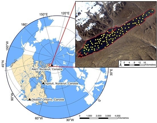
2. Study Area
3. Materials and Methods
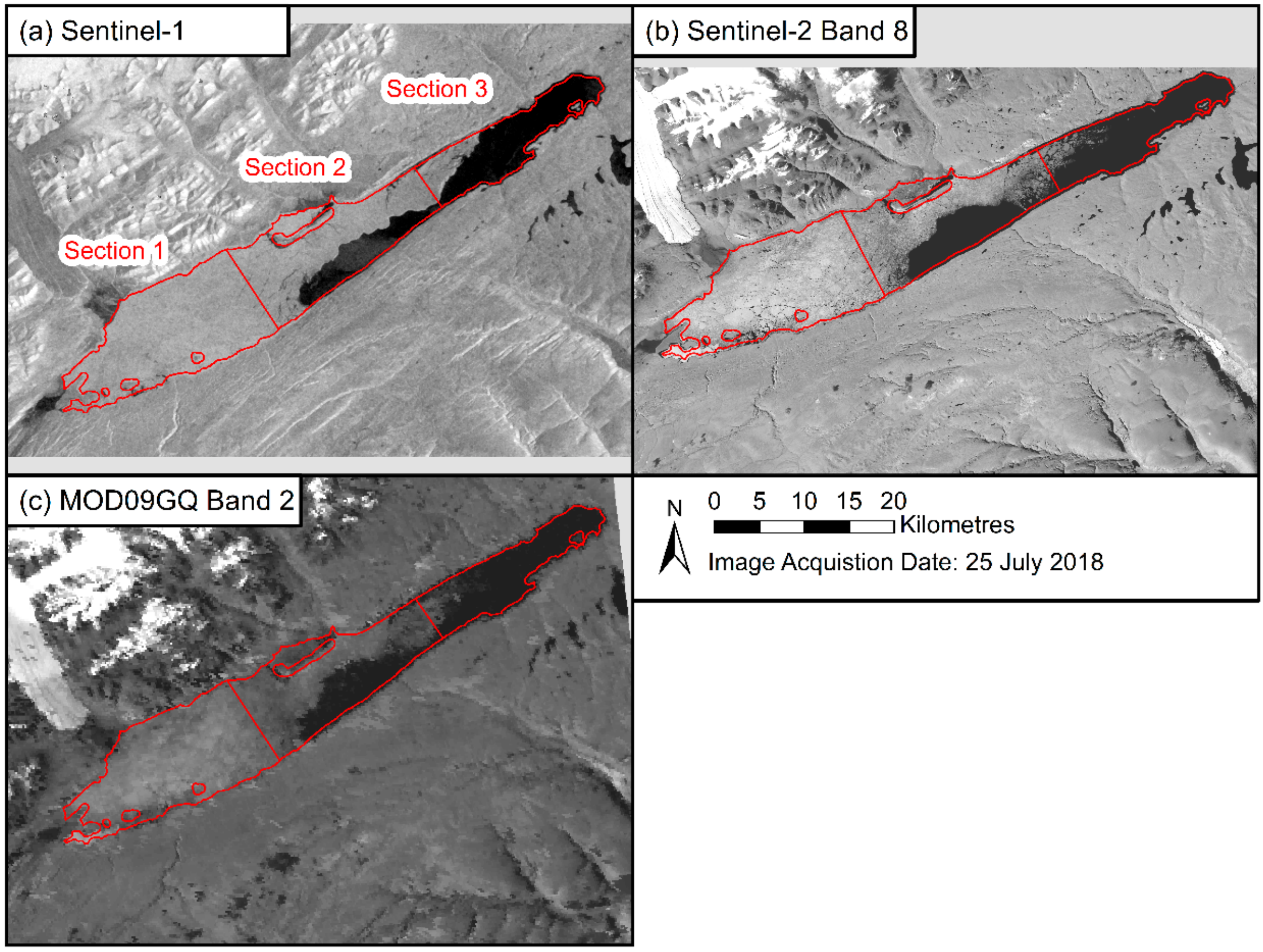
3.1. Sentinel-1 Data
3.2. Validation for Ice Phenology Dates
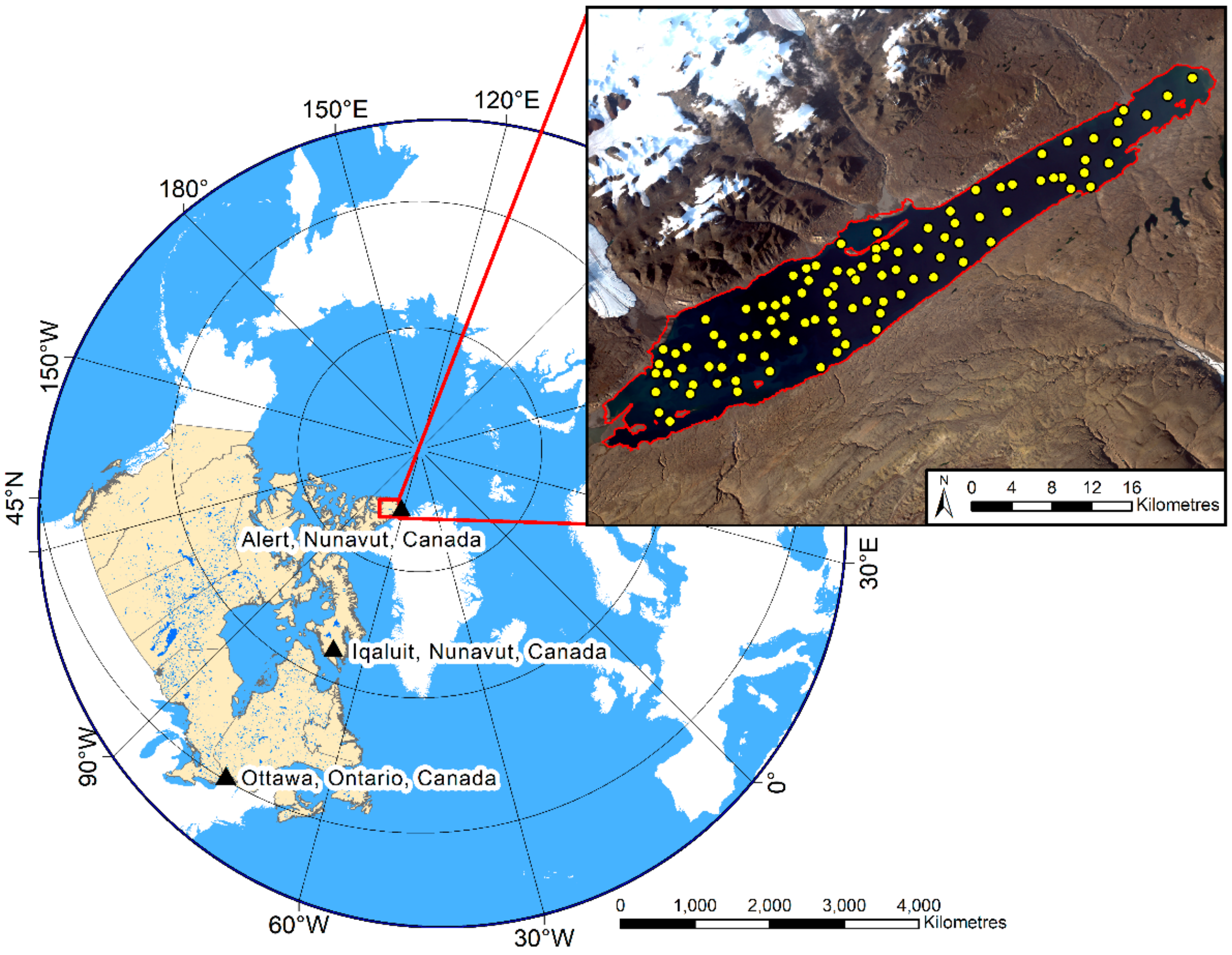
3.3. Lake Ice Detection Methods
3.3.1. Physical Basis of Backscatter Difference
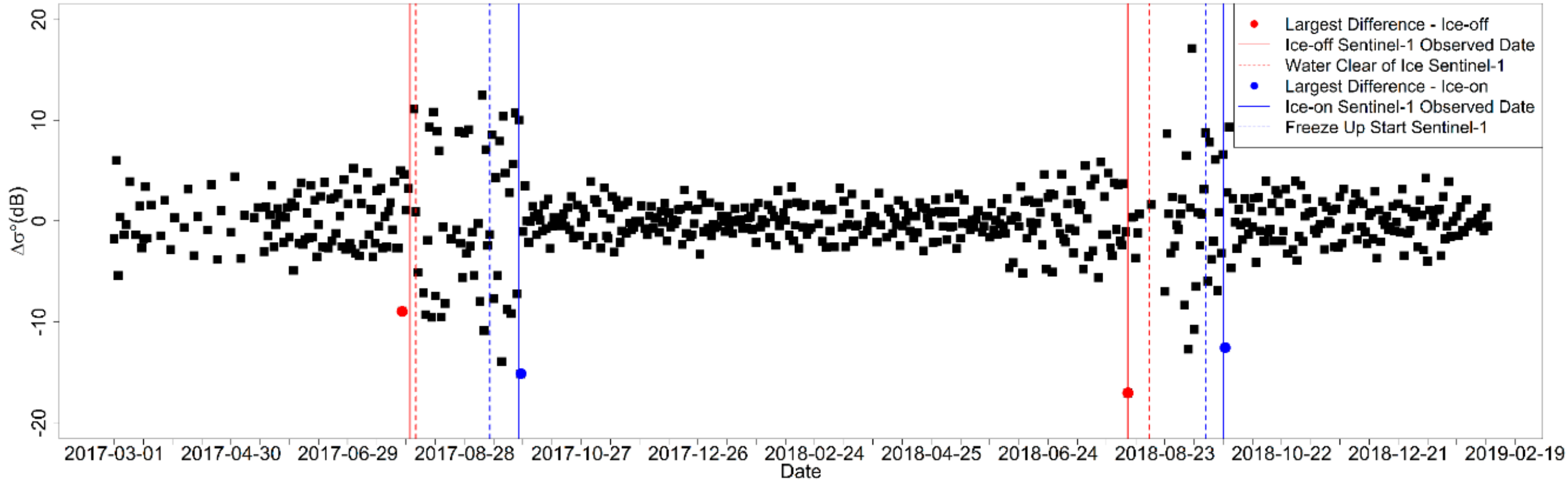
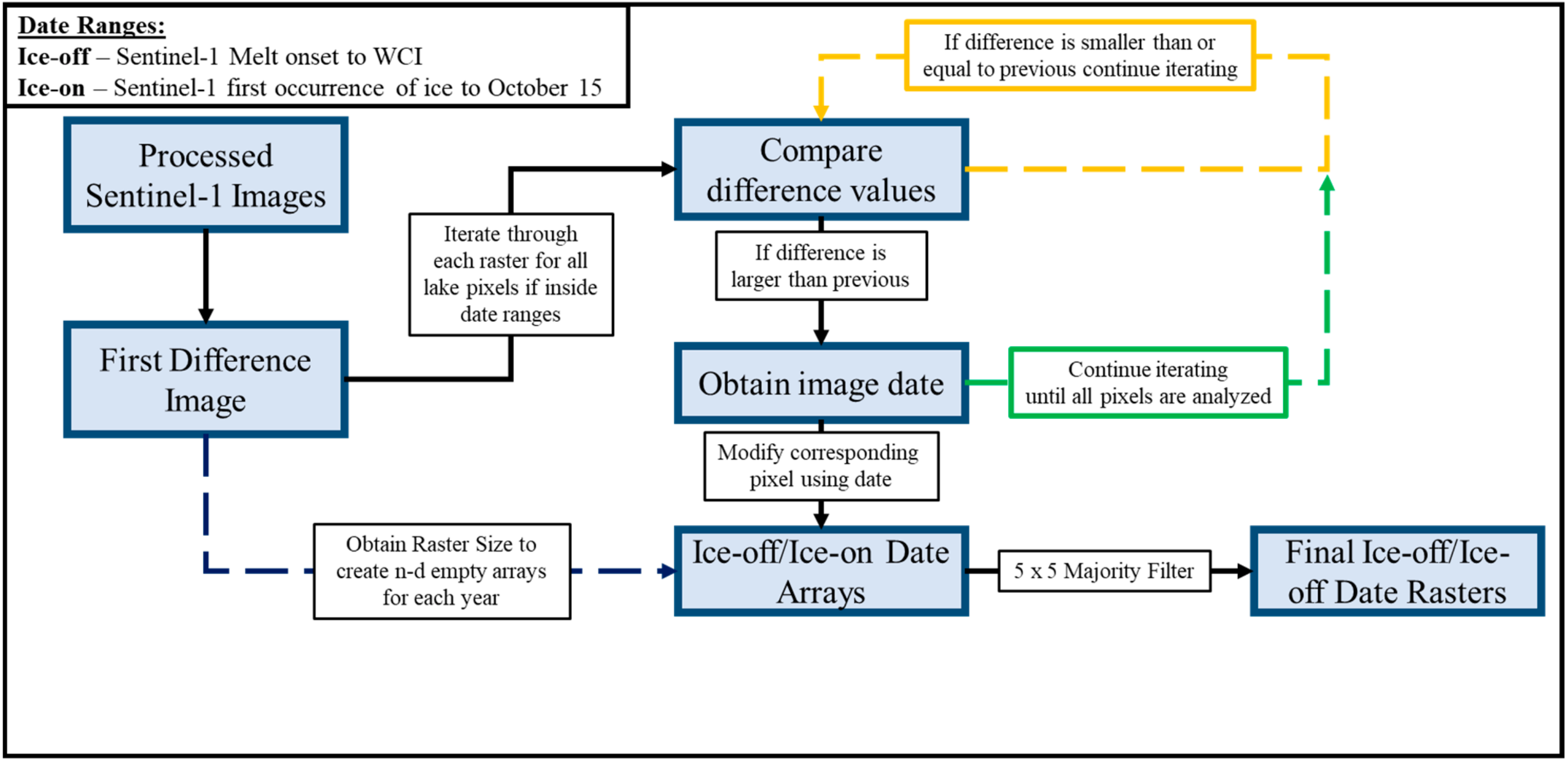
3.3.2. Identification of Lake Ice Phenology Using First Difference
3.3.3. Physical Basis of Two Class Segmentation
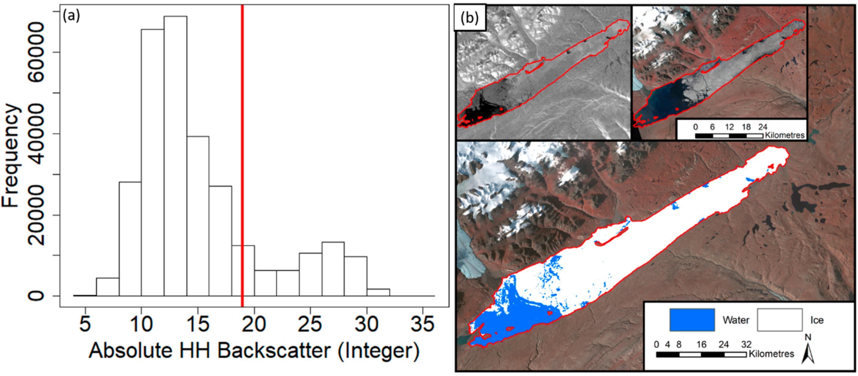
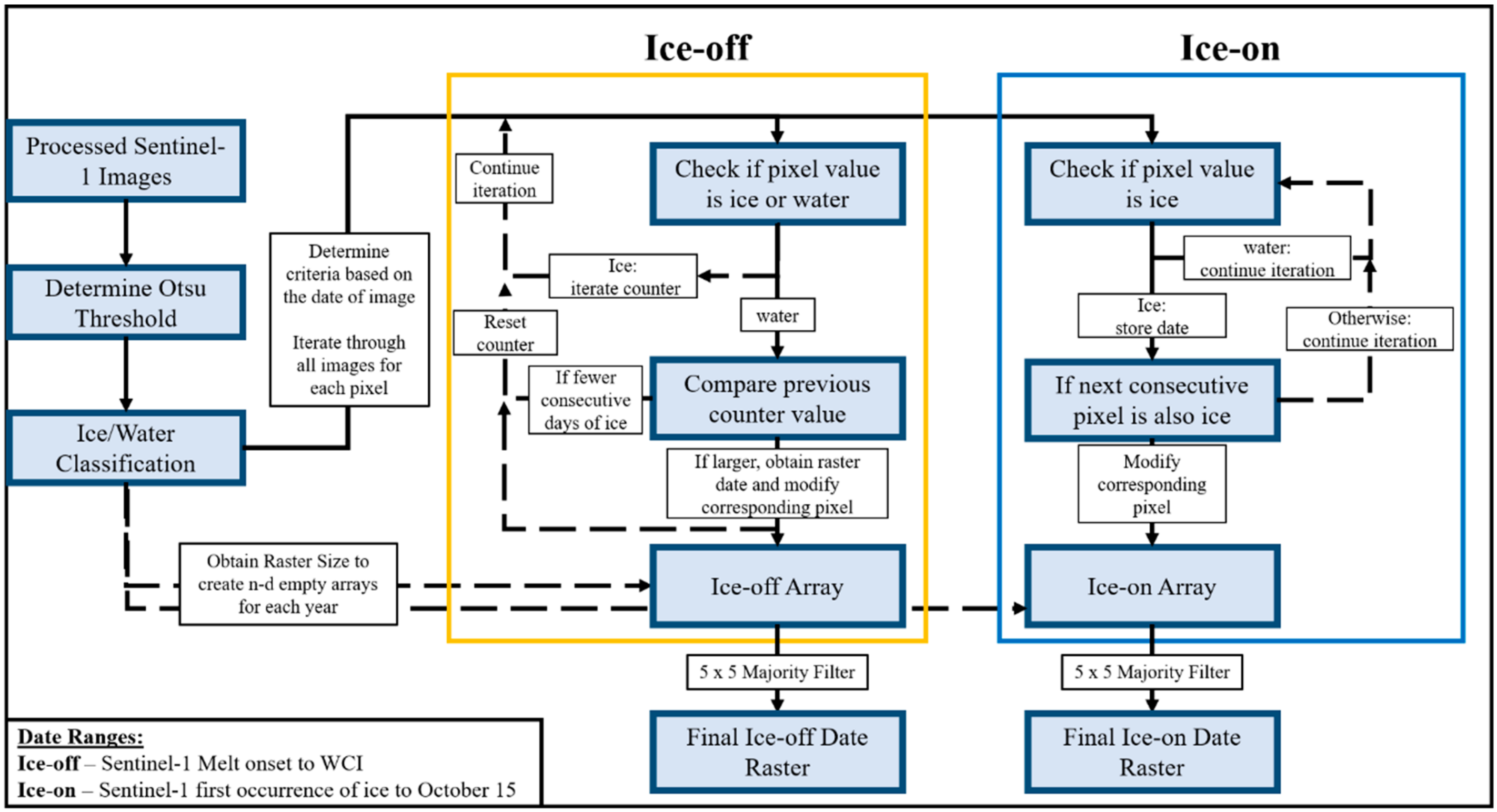
3.3.4. Identification of Lake Ice Phenology Using Otsu Segmentation
4. Results
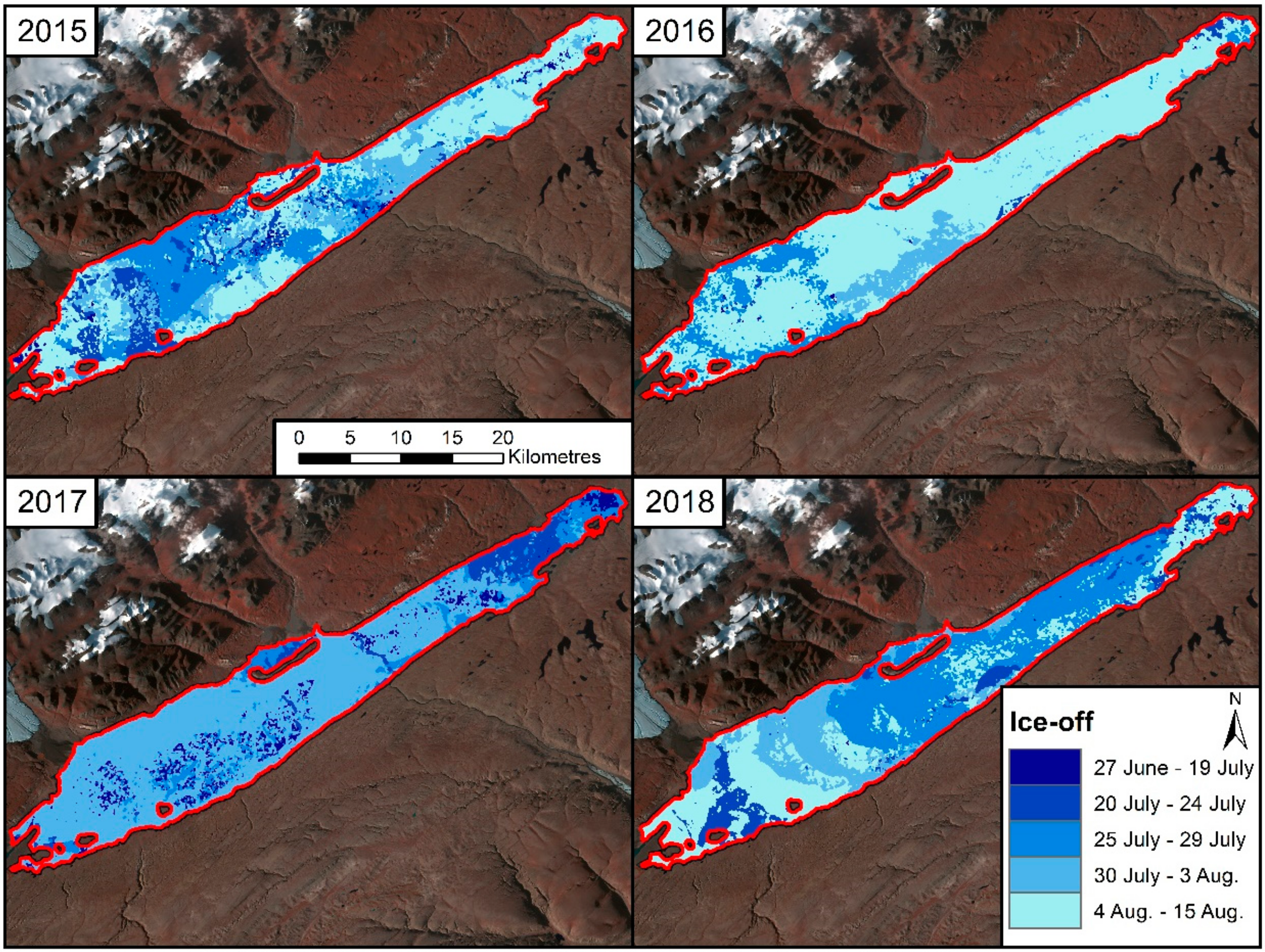
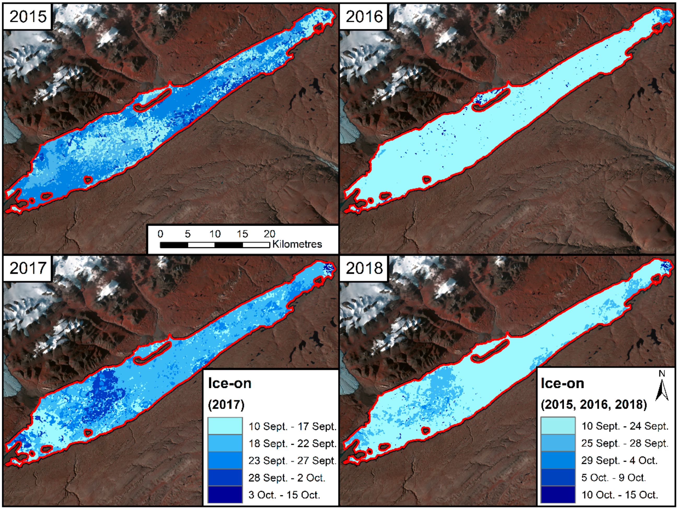
4.1. First Difference Lake Ice Phenology
4.1.1. Pixel-by-Pixel Comparison
4.1.2. Sectional Date Comparison
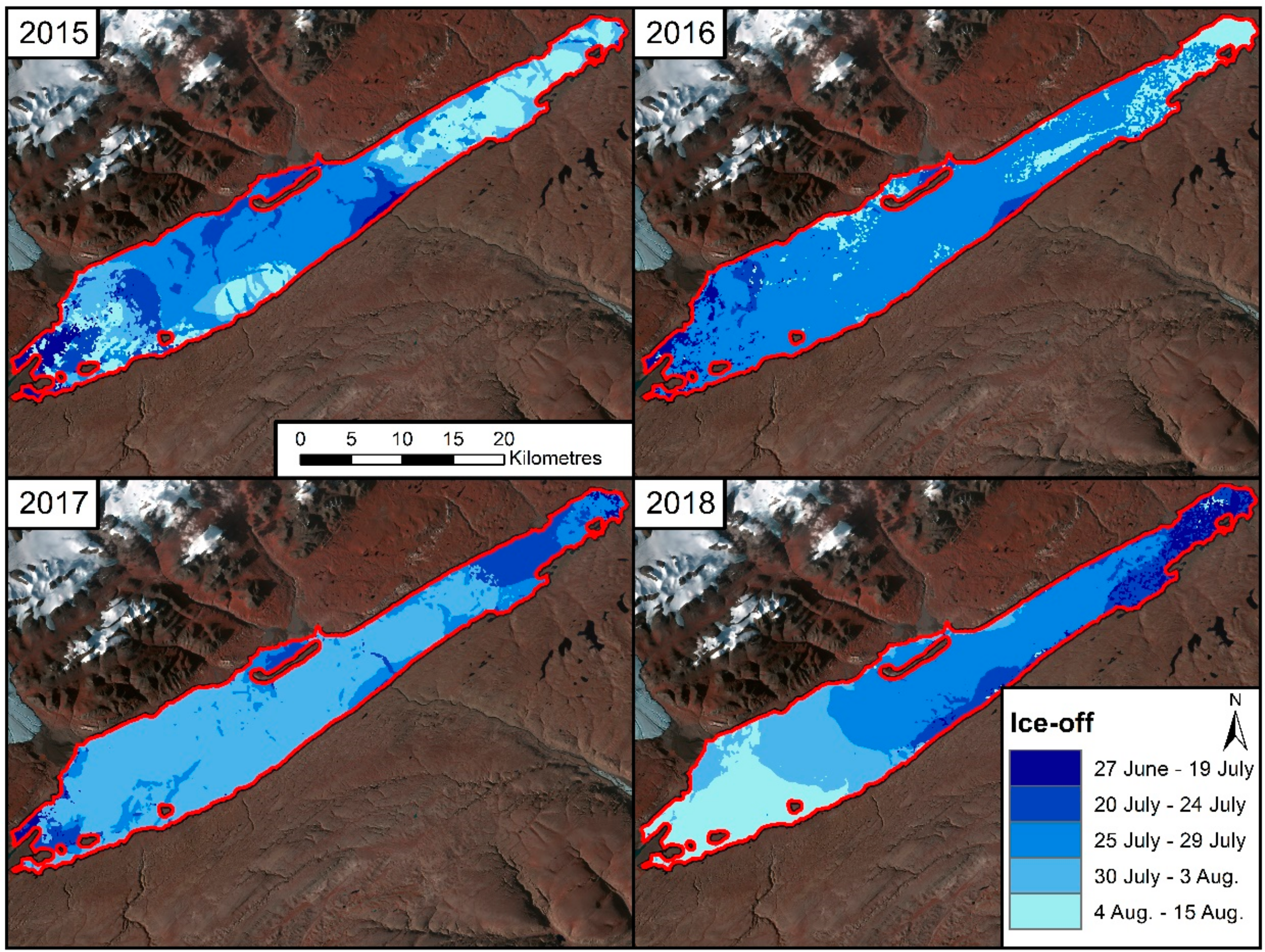
4.2. Otsu Segmentation
4.2.1. Pixel-by-Pixel Comparison
4.2.2. Sectional Date Comparison
5. Discussion
5.1. Sources of Error for the First Difference Method
5.2. Sources of Error for the Otsu Method
5.3. Comparison of the Methods
6. Conclusions
Supplementary Materials
Author Contributions
Funding
Acknowledgments
Conflicts of Interest
References
- Duguay, C.R.; Flato, G.M.; Jeffries, M.O.; Ménard, P.; Morris, K.; Rouse, W.R. Ice-Cover Variability on Shallow Lakes at High Latitudes: Model Simulations and Observations. Hydrol. Process. 2003, 17, 3465–3483. [Google Scholar] [CrossRef]
- Rouse, W.R.; Binyamin, J.; Blanken, P.D.; Bussières, N.; Duguay, C.R.; Oswald, C.J.; Schertzer, W.M.; Spence, C. The Influence of Lakes on the Regional Energy and Water Balance of the Central Mackenzie. In Cold Region Atmospheric and Hydrologic Studies: The Mackenzie GEWEX Experience Volume 1: Atmospheric Dynamics; Woo, M., Ed.; Springer: Berlin/Heidelberg, Germany; New York, NY, USA, 2008; pp. 309–325. [Google Scholar]
- Rouse, W.R.; Blanken, P.D.; Duguay, C.R.; Oswald, C.J.; Schertzer, W.M. Climate-Lake Interactions. In Cold Region Atmospheric and Hydrologic Studies: The Mackenzie GEWEX Experience Volume 2: Hydrologic Processes; Woo, M., Ed.; Springer: Berlin/Heidelberg, Germany; New York, NY, USA, 2008; pp. 139–160. [Google Scholar]
- Šmejkalová, T.; Edwards, M.E.; Dash, J. Arctic Lakes Show Strong Decadal Trend in Earlier Spring Ice-Out. Sci. Rep. 2016, 6, 1–8. [Google Scholar] [CrossRef] [PubMed]
- Brown, L.C.; Duguay, C.R. The Fate of Lake Ice in the North American Arctic. Cryosph. 2011, 5, 869–892. [Google Scholar] [CrossRef]
- Dibike, Y.; Prowse, T.; Bonsal, B.; Rham, L.D.; Saloranta, T. Simulation of North American Lake-Ice Cover Characteristics under Contemporary and Future Climate Conditions. Int. J. Climatol. 2012, 32, 695–709. [Google Scholar] [CrossRef]
- Cohen, J.; Screen, J.A.; Furtado, J.C.; Barlow, M.; Whittleston, D.; Coumou, D.; Francis, J.; Dethloff, K.; Entekhabi, D.; Overland, J.; et al. Recent Arctic Amplification and Extreme Mid-Latitude Weather. Nat. Geosci. 2014, 7, 627–637. [Google Scholar] [CrossRef]
- Mullan, D.; Swindles, G.; Patterson, T.; Galloway, J.; Macumber, A.; Falck, H.; Crossley, L.; Chen, J.; Pisaric, M. Climate Change and the Long-Term Viability of the World’s Busiest Heavy Haul Ice Road. Theor. Appl. Climatol. 2017, 129, 1089–1108. [Google Scholar] [CrossRef]
- Knoll, L.B.; Sharma, S.; Denfeld, B.A.; Flaim, G.; Hori, Y.; Magnuson, J.J.; Straile, D.; Weyhenmeyer, G.A. Consequences of Lake and River Ice Loss on Cultural Ecosystem Services. Limnol. Oceanogr. Lett. 2019, 4, 119–131. [Google Scholar] [CrossRef]
- Özkundakci, D.; Gsell, A.S.; Hintze, T.; Täuscher, H.; Adrian, R. Winter Severity Determines Functional Trait Composition of Phytoplankton in Seasonally Ice-Covered Lakes. Glob. Chang. Biol. 2016, 22, 284–298. [Google Scholar] [CrossRef]
- Hampton, S.E.; Galloway, A.W.E.; Powers, S.M.; Ozersky, T.; Woo, K.H.; Batt, R.D.; Labou, S.G.; O’Reilly, C.M.; Sharma, S.; Lottig, N.R.; et al. Ecology Under Lake Ice. Ecol. Lett. 2017, 20, 98–111. [Google Scholar] [CrossRef]
- Preston, D.L.; Caine, N.; McKnight, D.M.; Williams, M.W.; Hell, K.; Miller, M.P.; Hart, S.J.; Johnson, P.T.J. Climate regulates alpine lake ice cover phenology and aquatic ecosystem structure. Geophys. Res. Lett. 2016, 43, 5353–5360. [Google Scholar] [CrossRef]
- Lenormand, F.; Duguay, C.R.; Gauthier, R. Development of a Historical Ice Database for the Study of Climate Change in Canada. Hydrol. Process. 2002, 16, 3707–3722. [Google Scholar] [CrossRef]
- Duguay, C.R.; Bernier, M.; Gauthier, Y.; Kouraev, A. Remote Sensing of Lake and River Ice. In Remote Sensing of the Cryosphere; Tedesco, M., Ed.; John Wiley & Sons, Ltd.: Hoboken, NJ, USA, 2015; pp. 273–306. [Google Scholar]
- Reed, B.; Budde, M.; Spencer, P.; Miller, A.E. Integration of MODIS-Derived Metrics to Assess Interannual Variability in Snowpack, Lake Ice, and NDVI in Southwest Alaska. Remote Sens. Environ. 2009, 113, 1443–1452. [Google Scholar] [CrossRef]
- Arp, C.D.; Jones, B.M.; Grosse, G. Recent Lake Ice-Out Phenology within and among Lake Districts of Alaska, U.S.A. Limnol. Oceanogr. 2013, 58, 2013–2028. [Google Scholar] [CrossRef]
- Surdu, C.M.; Duguay, C.R.; Brown, L.C.; Prieto, D.F. Response of Ice Cover on Shallow Lakes of the North Slope of Alaska to Contemporary Climate Conditions (1950–2011): Radar Remote-Sensing and Numerical Modeling Data Analysis. Cryosphere 2014, 8, 167–180. [Google Scholar] [CrossRef]
- Surdu, C.M.; Duguay, C.R.; Prieto, D.F. Evidence of Recent Changes in the Ice Regime of Lakes in the Canadian High Arctic from Spaceborne Satellite Observations. Cryosphere 2016, 10, 941–960. [Google Scholar] [CrossRef]
- Murfitt, J.; Brown, L.C.; Howell, S.E.L. Evaluating RADARSAT-2 for the Monitoring of Lake Ice Phenology Events in Mid-Latitudes. Remote Sens. 2018, 10, 1641. [Google Scholar] [CrossRef]
- Hall, D.K.; Fagre, D.B.; Klasner, F.; Linebaugh, G.; Liston, G.E. Analysis of ERS 1 Synthetic Aperture Radar Data of Frozen Lakes in Northern Montana and Implications for Climate Studies. J. Geophys. Res. 1994, 99, 22473–22482. [Google Scholar] [CrossRef]
- Duguay, C.R.; Pultz, T.J.; Lafleur, P.M.; Drai, D. RADARSAT Backscatter Characteristics of Ice Growing on Shallow Sub-Arctic Lakes, Churchill, Manitoba, Canada. Hydrol. Process. 2002, 16, 1631–1644. [Google Scholar] [CrossRef]
- Weeks, W.F.; Fountain, A.G.; Bryan, M.L.; Elachi, C. Differences in Radar Return From Ice-Covered North Slope Lakes. J. Geophys. Res. 1978, 83, 4069–4073. [Google Scholar] [CrossRef]
- Surdu, C.M.; Duguay, C.R.; Pour, H.K.; Brown, L.C. Ice Freeze-up and Break-up Detection of Shallow Lakes in Northern Alaska with Spaceborne SAR. Remote Sens. 2015, 7, 6133–6159. [Google Scholar] [CrossRef]
- Jeffries, M.O.; Morris, K.; Weeks, W.F.; Wakabayashi, H. Structural and Stratigraphic Features and ERS 1 Synthetic Aperture Radar Backscatter Characteristics of Ice Growing on Shallow Lakes in NW Alaska, Winter 1991-1992. J. Geophys. Res. 1994, 99, 22459–22471. [Google Scholar] [CrossRef]
- Morris, K.; Jeffries, M.O.; Weeks, W.F. Ice Processes and Growth History on Arctic and Sub-Arctic Lakes using ERS-1 SAR Data. Polar Rec. (Gr. Brit). 1995, 31, 115–128. [Google Scholar] [CrossRef]
- Howell, S.E.L.; Brown, L.C.; Kang, K.-K.; Duguay, C.R. Variability in Ice Phenology on Great Bear Lake and Great Slave Lake, Northwest Territories, Canada, from SeaWinds/QuikSCAT: 2000–2006. Remote Sens. Environ. 2009, 113, 816–834. [Google Scholar] [CrossRef]
- Sobiech, J.; Dierking, W. Observing Lake and River-Ice Decay with SAR: Advantages and Limitations of the Unsupervised K-Means Classification Approach. Ann. Glaciol. 2013, 54, 65–72. [Google Scholar] [CrossRef]
- Xiao, M.; Rothermel, M.; Tom, M.; Galliani, S.; Baltsavias, E.; Schindler Photogrammetry, K.; Sensing, R.; Zürich, E. Lake Ice Monitoring with Webcams. ISPRS Ann. Photogramm. Remote Sens. Spat. Inf. Sci. 2018, IV–2, 311–317. [Google Scholar] [CrossRef]
- Wang, J.; Duguay, C.R.; Clausi, D.A.; Pinard, V.; Howell, S.E.L. Semi-Automated Classification of Lake Ice Cover Using Dual Polarization RADARSAT-2 Imagery. Remote Sens. 2018, 10, 1727. [Google Scholar] [CrossRef]
- Geldsetzer, T.; van der Sanden, J.; Brisco, B. Monitoring Lake Ice During Spring Melt using RADARSAT-2 SAR. Can. J. Remote Sens. 2010, 36, 391–400. [Google Scholar] [CrossRef]
- Geldsetzer, T.; van der Sanden, J.J. Identification of Polarimetric and Nonpolarimetric C-band SAR Parameters for Application in the Monitoring of Lake Ice Freeze-up. Can. J. Remote Sens. 2013, 39, 263–275. [Google Scholar] [CrossRef]
- Howell, S.E.L.; Small, D.; Rohner, C.; Mahmud, M.S.; Yackel, J.J.; Brady, M. Estimating Melt Onset over Arctic Sea Ice from Time Series Multi-sensor Sentinel-1 and RADARSAT-2 Backscatter. Remote Sens. Environ. 2019, 229, 48–59. [Google Scholar] [CrossRef]
- Herdendorf, C.E. Large Lakes of the World. J. Great Lakes Res. 1982, 8, 379–412. [Google Scholar] [CrossRef]
- Environment and Climate Change Canada Alert Climate Normals 1981–2010. Available online: http://climate.weather.gc.ca/climate_normals/results_1981_2010_e.html?stnID=1731&autofwd=1 (accessed on 14 August 2019).
- National Oceanic and Atmospheric Administration: Earth System Research Laboratory - Global Monitoring Division Sunrise/Sunset Calculator. Available online: https://www.esrl.noaa.gov/gmd/grad/solcalc/ (accessed on 24 December 2019).
- Köck, A.G.; Muir, D.; Yang, F.; Wang, X.; Talbot, C.; Gantner, N.; Moser, D. Bathymetry and Sediment Geochemistry of Lake Hazen (Quttinirpaaq National Park, Ellesmere Island, Nunavut). Arctic 2012, 65, 56–66. [Google Scholar] [CrossRef]
- Lehnherr, I.; Louis, V.L.S.; Sharp, M.; Gardner, A.S.; Smol, J.P.; Schiff, S.L.; Muir, D.C.G.; Mortimer, C.A.; Michelutti, N.; Tarnocai, C.; et al. The World’s Largest High Arctic Lake Responds Rapidly to Climate Warming. Nat. Commun. 2018, 9, 1–9. [Google Scholar] [CrossRef] [PubMed]
- St. Pierre, K.A.; St. Louis, V.L.; Lehnherr, I.; Schiff, S.L.; Muir, D.C.G.; Poulain, A.J.; Smol, J.P.; Talbot, C.; Ma, M.; Findlay, D.L.; et al. Contemporary Limnology of the Rapidly Changing Glacierized Watershed of the World’s Largest High Arctic lake. Sci. Rep. 2019, 9, 4447. [Google Scholar]
- Copernicus Sentinel-1 data (2014 to 2019). Retrieved from ASF DAAC (7/02/2019), Processed by ESA. Available online: https://www.asf.alaska.edu/ (accessed on 2 July 2019).
- European Space Agency SNAP. ESA Sentinel Application Platform v6.0 2019; ESA: Paris, France, 2019. [Google Scholar]
- Lee, J. Refined Filtering of Image Noise Using Local Statistics. Comput. Graph. Image Process. 1981, 15, 380–389. [Google Scholar] [CrossRef]
- GDAL/OGR Contributors. GDAL/OGR Geospatial Data Abstraction Software Library; Open Source Geospatial Foundation: Chicago, IL, USA, 2019. [Google Scholar]
- Porter, C.; Morin, P.; Howat, I.; Noh, M.-J.; Bates, B.; Peterman, K.; Keesey, S.; Schlenk, M.; Gardiner, J.; Tomko, K.; et al. ArcticDEM, V1. Available online: https://dataverse.harvard.edu/dataset.xhtml?persistentId=doi:10.7910/DVN/OHHUKH (accessed on 22 May 2019).
- Mäkynen, M.P.; Manninen, A.T.; Similä, M.H.; Karvonen, J.A.; Hallikainen, M.T. Incidence Angle Dependence of the Statistical Properties of C-Band HH-Polarization Backscattering Signatures of the Baltic Sea Ice. IEEE Trans. Geosci. Remote Sens. 2002, 40, 2593–2605. [Google Scholar] [CrossRef]
- Mahmud, M.S.; Howell, S.E.L.; Geldsetzer, T.; Yackel, J. Detection of Melt Onset over the Northern Canadian Arctic Archipelago Sea Ice from RADARSAT, 1997 – 2014. Remote Sens. Environ. 2016, 178, 59–69. [Google Scholar] [CrossRef]
- Isoguchi, O.; Shimada, M. An L-band Ocean Geophysical Model Function Derived from PALSAR. IEEE Trans. Geosci. Remote Sens. 2009, 47, 1925–1936. [Google Scholar] [CrossRef]
- Pogson, L.; Geldsetzer, T.; Buehner, M.; Carrieres, T.; Ross, M.; Scott, K.A. Collecting Empirically Derived SAR Characteristic Values over One Year of Sea Ice Environments for Use in Data Assimilation. Mon. Weather Rev. 2017, 145, 323–334. [Google Scholar] [CrossRef]
- Wolfe, V.E. MOD09GQ MODIS/Terra Surface Reflectance Daily L2G Global 250m SIN Grid V006 [Data Set]. Available online: https://doi.org/10.5067/MODIS/MOD09GQ.006 (accessed on 9 May 2019).
- Willmott, C.J.; Matsuura, K. Advantages of the Mean Absolute Error (MAE) over the Root Mean Square Error (RMSE) in Assessing Average Model Performance. Clim. Res. 2005, 30, 79–82. [Google Scholar] [CrossRef]
- Leconte, R.; Klassen, P.D. Lake and River Ice Investigations in Northern Manitoba Using Airborne SAR Imagery. Arctic 1991, 44, 153–163. [Google Scholar] [CrossRef]
- Elachi, C.; Bryan, M.L.; Weeks, W.F. Imaging Radar Observations of Frozen Arctic Lakes. Remote Sens. Environ. 1976, 5, 169–175. [Google Scholar] [CrossRef]
- Weeks, W.F.; Sellmann, P.; Campbell, W.J. Interesting Features of Radar Imagery of Ice Covered North Slope Lakes. J. Glaciol. 1977, 18, 129–136. [Google Scholar] [CrossRef]
- Atwood, D.K.; Gunn, G.E.; Roussi, C.; Wu, J.; Duguay, C.; Sarabandi, K. Microwave Backscatter from Arctic Lake Ice and Polarimetric Implications. IEEE Trans. Geosci. Remote Sens. 2015, 53, 5972–5982. [Google Scholar] [CrossRef]
- Gunn, G.E.; Duguay, C.R.; Atwood, D.K.; King, J.; Toose, P. Observing Scattering Mechanisms of Bubbled Freshwater Lake Ice Using Polarimetric RADARSAT-2 (C-Band) and UW-Scat (X- and Ku-Bands). IEEE Trans. Geosci. Remote Sens. 2018, 56, 2887–2903. [Google Scholar] [CrossRef]
- Torres, R.; Snoeij, P.; Geudtner, D.; Bibby, D.; Davidson, M.; Attema, E.; Potin, P.; Rommen, B.Ö.; Floury, N.; Brown, M.; et al. GMES Sentinel-1 Mission. Remote Sens. Environ. 2012, 120, 9–24. [Google Scholar] [CrossRef]
- Lindsay, J.B. WhiteboxTools User Manual. Available online: https://jblindsay.github.io/wbt_book/preface.html (accessed on 1 August 2019).
- Duguay, C.R.; Lafleur, P.M. Determining Depth and Ice Thickness of Shallow Sub-Arctic Lakes using Space-Borne Optical and SAR Data. Int. J. Remote Sens. 2003, 24, 475–489. [Google Scholar] [CrossRef]
- Kalke, H.; Loewen, M. Support Vector Machine Learning Applied to Digital Images of River Ice Conditions. Cold Reg. Sci. Technol. 2018, 155, 225–236. [Google Scholar] [CrossRef]
- Zhang, Q.; Skjetne, R.; Løset, S.; Marchenko, A. Digital Image Processing for Sea Ice Observations in Support to Arctic DP Operations. In Proceedings of the ASME 2012 31st International Conference on Ocean, Offshore and Arctic Engineering, Rio de Janeiro, Brazil, 1–6 July 2012; pp. 1–7. [Google Scholar]
- Zhang, Q.; van der Werff, S.; Metrikin, I.; Løset, S.; Skjetne, R. Image Processing for the Analysis of an Evolving Broken-Ice Field in Model Testing. In Proceedings of the ASME 2012 31st International Conference on Ocean, Offshore and Arctic Engineering, Rio de Janeiro, Brazil, 1–6 July 2012; pp. 1–8. [Google Scholar]
- Ji, Y.; Zhang, J.; Meng, J.; Zhang, X. Sea Ice Detection and Classification in Liadong Bay with Envisat ASAR Imagery. In Proceedings of the SeaSAR 2008, Frascati, Roma, Italy, 21–25 January 2008; p. 4. [Google Scholar]
- Otsu, N. A Threshold Selection Method from Gray-Level Histograms. IEEE Trans. Syst. Man. Cybern. 1979, 9, 62–66. [Google Scholar] [CrossRef]
- Du, J.; Kimball, J.S.; Duguay, C.; Kim, Y.; Watts, J.D. Satellite Microwave Assessment of Northern Hemisphere Lake Ice Phenology from 2002 to 2015. Cryosphere 2017, 11, 47–63. [Google Scholar] [CrossRef]
- Belward, A.; Bourassa, M.; Dowell, M.; Briggs, S.; Dolman, H.; Holmlund, K.; Verstraete, M. The Global Observing System for Climate: Implementation Needs. GCOS Steering Committee: Guayaquil, Ecuador. Ref. Number GCOS-200 2016, 315. [Google Scholar]
- Arkett, M.; Braithwaite, L.; Pestieau, P.; Carrieres, T.; Pogson, L.; Fabi, C.; Geldsetzer, T. Preparation by the Canadian Ice Service for the Operational Use of the RADARSAT Constellation Mission in Their Ice and Oil Spill Monitoring Programs. Can. J. Remote Sens. 2015, 41, 380–389. [Google Scholar] [CrossRef]


| Year | Melt Onset | Water Clear of Ice | Initial Ice Appearance |
|---|---|---|---|
| 2015 | 22 June | 9 August | 17 September |
| 2016 | 29 June | 14 August | 11 September |
| 2017 | 29 June | 3 August | 10 September |
| 2018 | 29 June | 15 August | 13 September |
| 2015 | 2016 | 2017 | 2018 | ||
|---|---|---|---|---|---|
| Ice-off | MBE | 1 | 3 | −4 | 0 |
| MAE | 5 | 4 | 5 | 3 | |
| Ice-on | MBE | −7 | −1 | −10 | −5 |
| MAE | 7 | 3 | 10 | 6 | |
| Water Clear of Ice (WCI) | Complete Freeze Over (CFO) | |||||||
|---|---|---|---|---|---|---|---|---|
| Sentinel-1 | Est. Date | Difference | Sentinel-1 | Est. Date | Difference | |||
| 2015 | ||||||||
| Section 1 | 217 | 210 | −7 | 280 | 269 | −11 | ||
| Section 2 | 217 | 214 | −3 | 280 | 274 | −6 | ||
| Section 3 | 221 | 217 | −4 | 280 | 269 | −11 | ||
| MBE: −5 days | MAE: 5 days | MBE: −10 days | MAE: 10 days | |||||
| 2016 | ||||||||
| Section 1 | 217 | 217 | 0 | 270 | 265 | −5 | ||
| Section 2 | 219 | 220 | 1 | 268 | 265 | −3 | ||
| Section 3 | 227 | 219 | −8 | 268 | 265 | −3 | ||
| MBE: −3 days | MAE: 3 days | MBE: −4 days | MAE: 4 days | |||||
| 2017 | ||||||||
| Section 1 | 214 | 212 | −2 | 269 | 259 | −10 | ||
| Section 2 | 215 | 212 | −3 | 270 | 255 | −15 | ||
| Section 3 | 215 | 207 | −8 | 270 | 262 | −8 | ||
| MBE: -5 days | MAE: 5 days | MBE: -11 days | MAE: 11 days | |||||
| 2018 | ||||||||
| Section 1 | 227 | 215 | −12 | 272 | 262 | −10 | ||
| Section 2 | 215 | 209 | −6 | 271 | 262 | −9 | ||
| Section 3 | 208 | 207 | −1 | 270 | 262 | −8 | ||
| MBE: −7 days | MAE: 7 days | MBE: −9 days | MAE: 9 days | |||||
| 2015 | 2016 | 2017 | 2018 | ||
|---|---|---|---|---|---|
| Ice-off | MBE | −3 | −7 | −2 | −2 |
| MAE | 4 | 7 | 2 | 2 | |
| Ice-on | MBE | −10 | −6 | −8 | −6 |
| MAE | 10 | 6 | 9 | 6 | |
| Water Clear of Ice | Complete Freeze Over | |||||||
|---|---|---|---|---|---|---|---|---|
| Sentinel-1 | Est. Date | Difference | Sentinel-1 | Est. Date | Difference | |||
| 2015 | ||||||||
| Section 1 | 217 | 208 | −9 | 280 | 264 | −16 | ||
| Section 2 | 217 | 210 | −7 | 280 | 269 | −11 | ||
| Section 3 | 221 | 218 | −3 | 280 | 269 | −11 | ||
| MBE: -7 days | MAE: 7 days | MBE: -13 days | MAE: 13 days | |||||
| 2016 | ||||||||
| Section 1 | 217 | 208 | −9 | 270 | 255 | −15 | ||
| Section 2 | 219 | 208 | −11 | 268 | 259 | −9 | ||
| Section 3 | 227 | 210 | −17 | 268 | 258 | −10 | ||
| MBE: −13 days | MAE: 13 days | MBE: −12 days | MAE: 12 days | |||||
| 2017 | ||||||||
| Section 1 | 214 | 212 | −2 | 269 | 259 | −10 | ||
| Section 2 | 215 | 212 | −3 | 270 | 262 | −8 | ||
| Section 3 | 215 | 207 | −8 | 270 | 257 | −13 | ||
| MBE: −5 days | MAE: 5 days | MBE: −11 days | MAE: 11 days | |||||
| 2018 | ||||||||
| Section 1 | 227 | 215 | −12 | 272 | 262 | −10 | ||
| Section 2 | 215 | 207 | −8 | 271 | 266 | −5 | ||
| Section 3 | 208 | 204 | −4 | 270 | 258 | −12 | ||
| MBE: −8 days | MAE: 8 days | MBE: −9 days | MAE: 9 days | |||||
© 2020 by the authors. Licensee MDPI, Basel, Switzerland. This article is an open access article distributed under the terms and conditions of the Creative Commons Attribution (CC BY) license (http://creativecommons.org/licenses/by/4.0/).
Share and Cite
Murfitt, J.; Duguay, C.R. Assessing the Performance of Methods for Monitoring Ice Phenology of the World’s Largest High Arctic Lake Using High-Density Time Series Analysis of Sentinel-1 Data. Remote Sens. 2020, 12, 382. https://doi.org/10.3390/rs12030382
Murfitt J, Duguay CR. Assessing the Performance of Methods for Monitoring Ice Phenology of the World’s Largest High Arctic Lake Using High-Density Time Series Analysis of Sentinel-1 Data. Remote Sensing. 2020; 12(3):382. https://doi.org/10.3390/rs12030382
Chicago/Turabian StyleMurfitt, Justin, and Claude R. Duguay. 2020. "Assessing the Performance of Methods for Monitoring Ice Phenology of the World’s Largest High Arctic Lake Using High-Density Time Series Analysis of Sentinel-1 Data" Remote Sensing 12, no. 3: 382. https://doi.org/10.3390/rs12030382
APA StyleMurfitt, J., & Duguay, C. R. (2020). Assessing the Performance of Methods for Monitoring Ice Phenology of the World’s Largest High Arctic Lake Using High-Density Time Series Analysis of Sentinel-1 Data. Remote Sensing, 12(3), 382. https://doi.org/10.3390/rs12030382