Discrepancy Analysis for Detecting Candidate Parcels Requiring Update of Land Category in Cadastral Map Using Hyperspectral UAV Images: A Case Study in Jeonju, South Korea


Abstract

1. Introduction
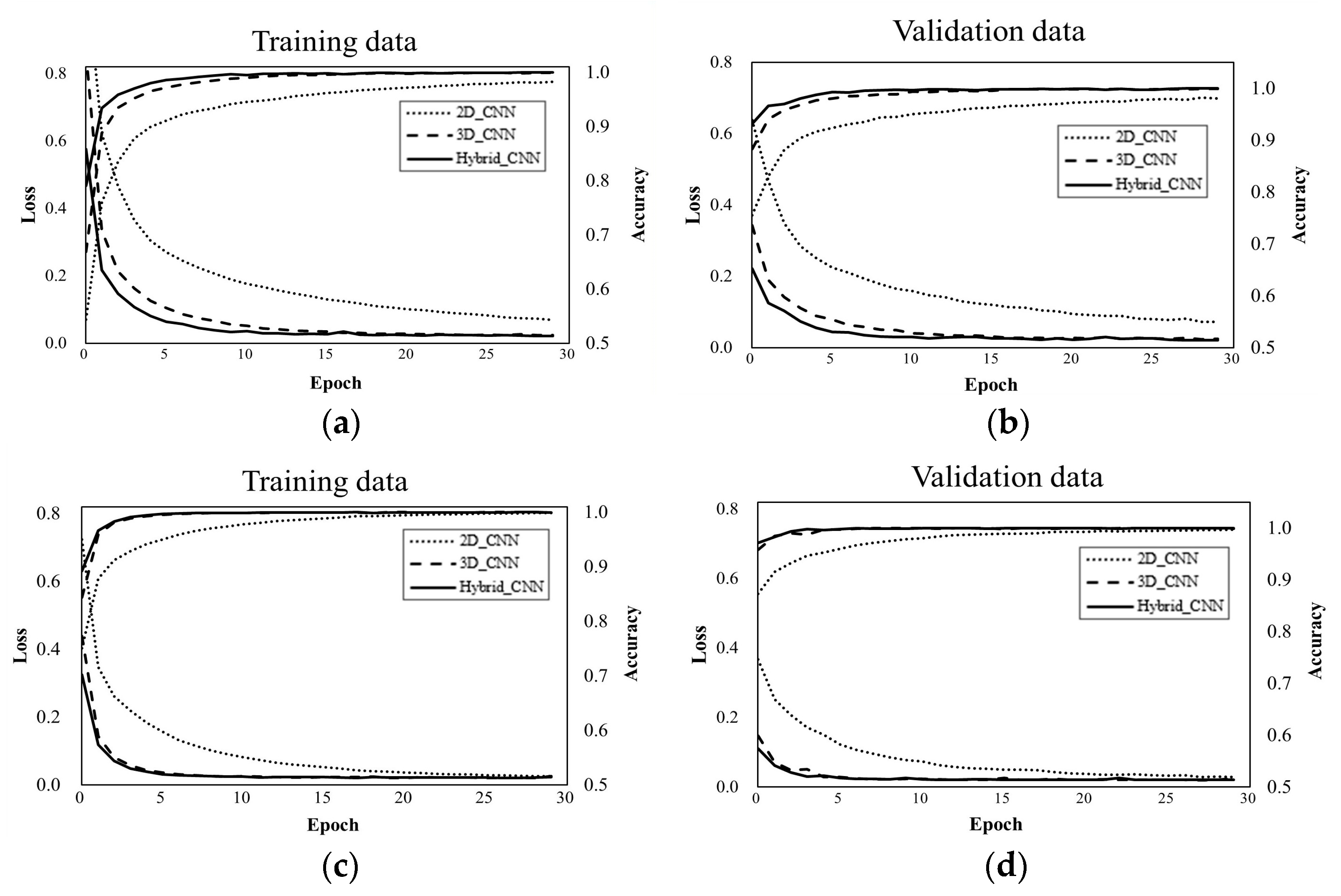
- For generating up-to-date land category information, we combine two-dimensional (2D) and three-dimensional (3D) convolutional neural networks (CNNs) to classify hyperspectral UAV images, and hence, generate the latest land category information at specific times and intervals. Furthermore, the environmental settings for learning are demonstrated and the classification results are analyzed to understand when the proposed network was applied to hyperspectral UAV images.
- For detecting discrepancies between the new information and the existing cadastral information, the efficiency of updating the registered land category is improved by a new technique that automatically compares two sets of non-spatial information under different criteria and structures.
2. Methods
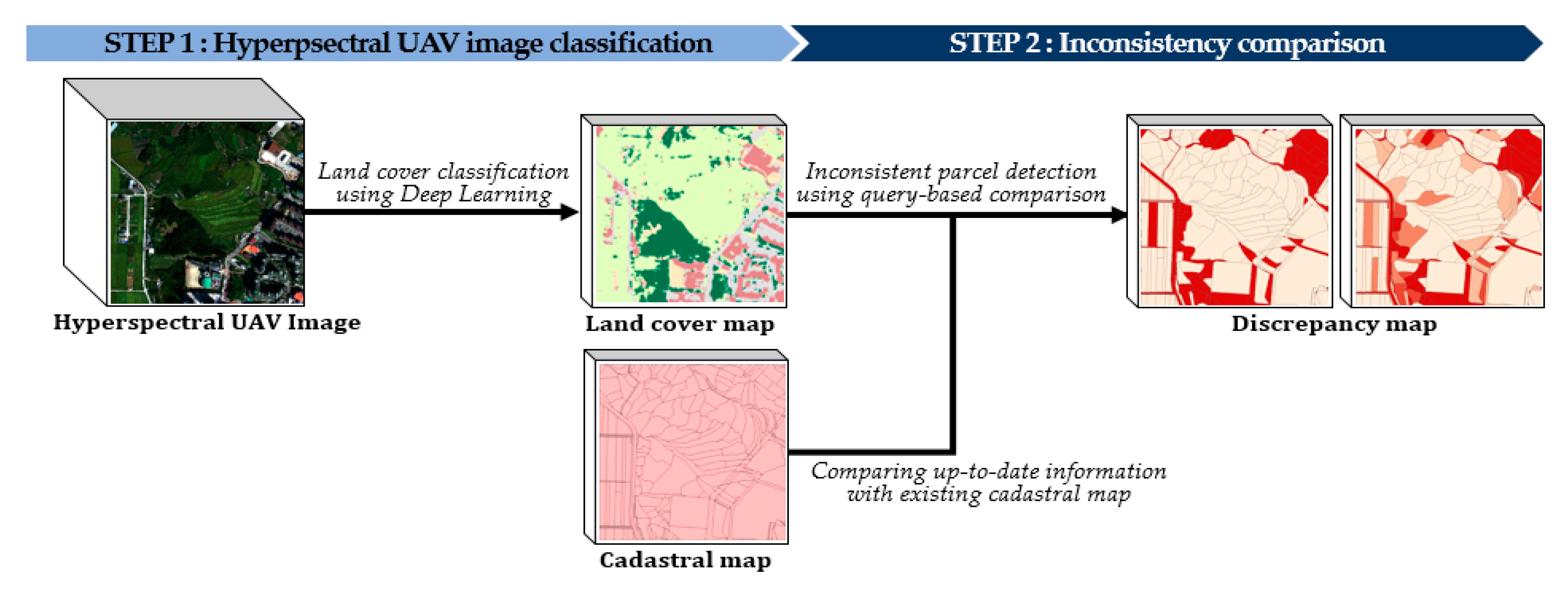
- (1)
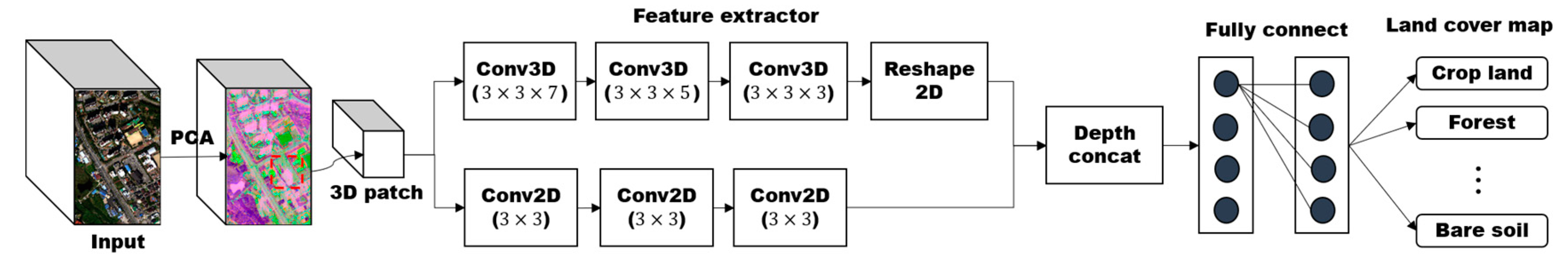
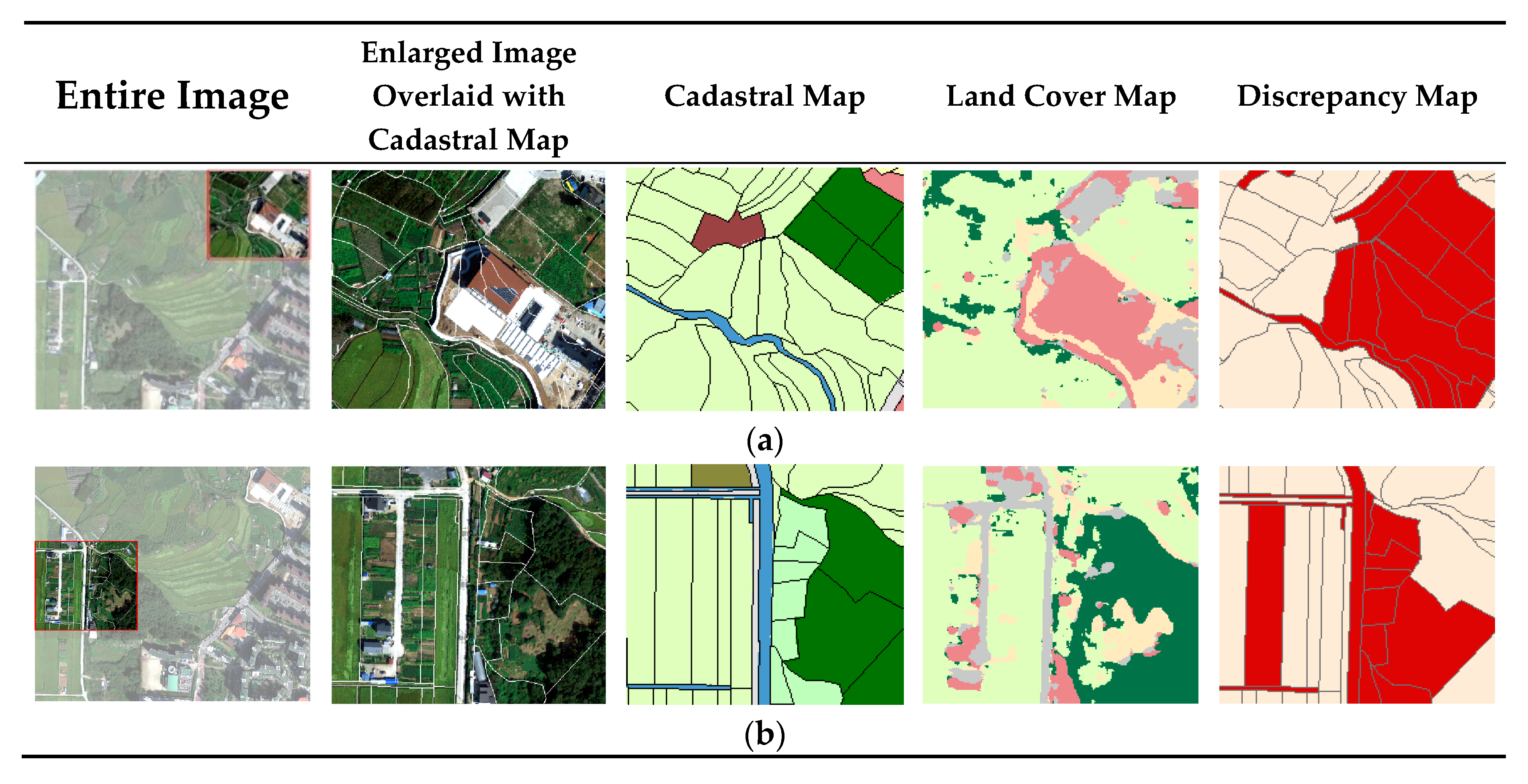
- The hybrid CNN with 2D and 3D kernels extracts the spatial–spectral features from hyperspectral UAV images and obtains a land cover map depicting the regions covered by forests, crops, bare soils, water, roads, and buildings. The images input to the hybrid CNN are pre-processed by principle component analysis (PCA) to reduce the number of redundant spectral bands and the computational cost. The hybrid CNN then classifies images by extracting various meaningful feature maps. The resulting land cover map provides the latest land information on sites.
- (2)
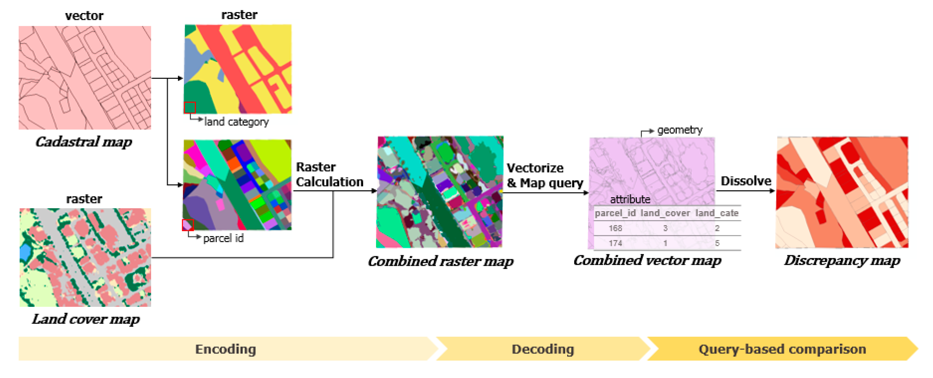
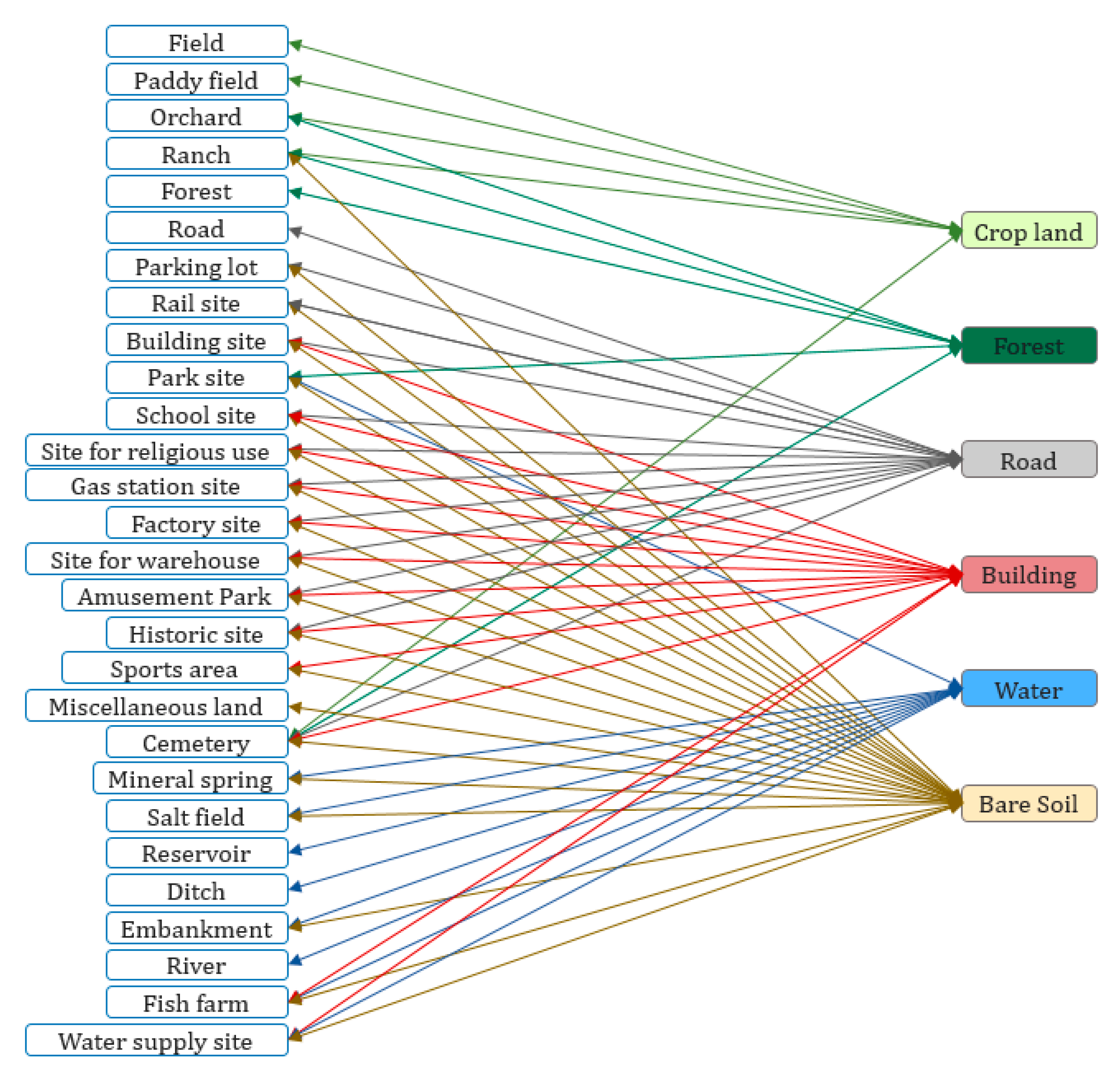
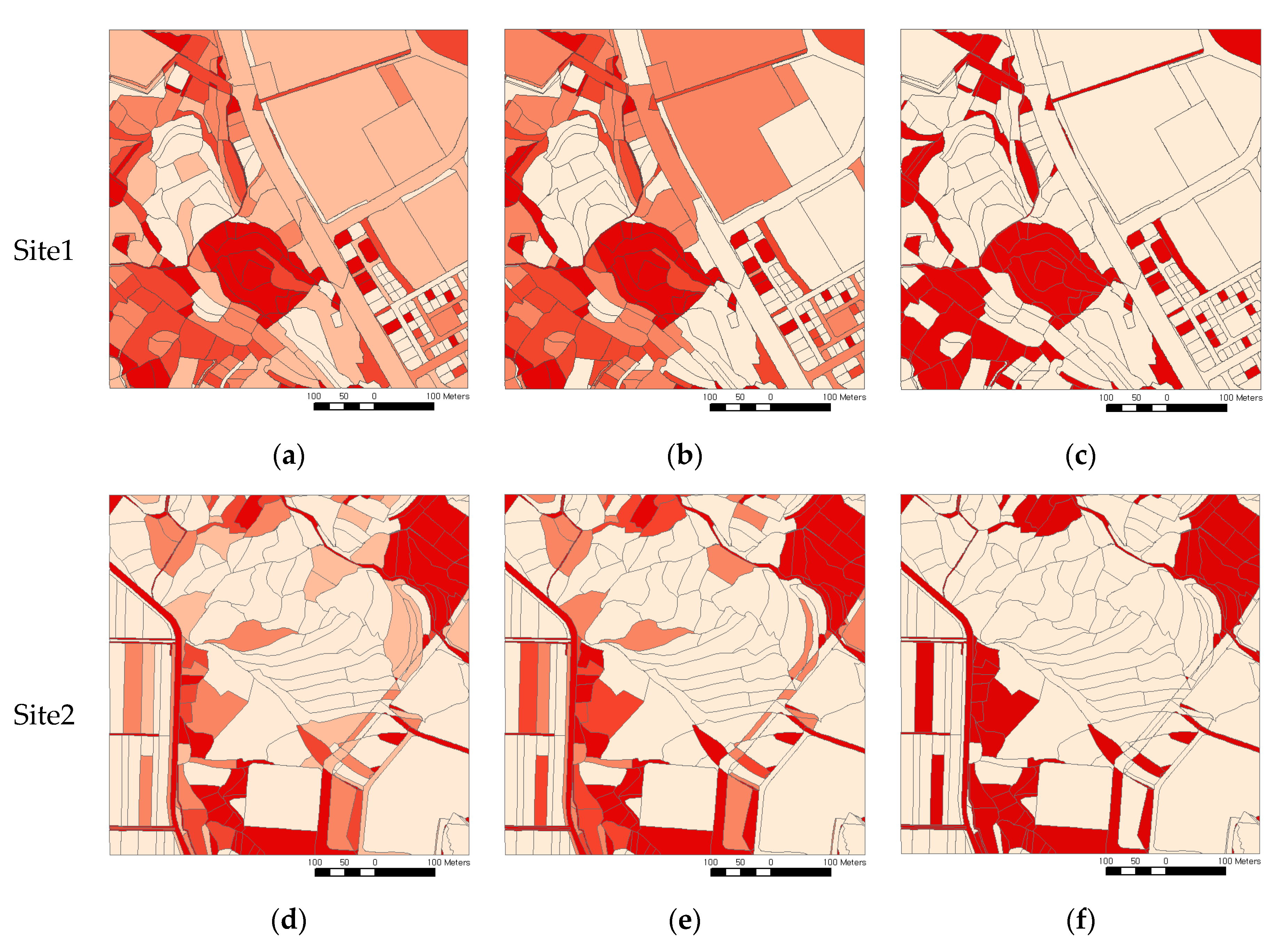
- To the procedure that automatically detects inconsistent parcels, two maps are input: the existing cadastral map, which is managed by the government, and the land cover map, which is generated from hyperspectral UAV image classification. To compare the heterogeneous datasets with vector and raster structured data, the procedure adopts an encoding–decoding approach. The final output is a discrepancy map generated through query-based comparison of the mapping information in the land category items and the land cover classes in different frameworks.
2.1. Step 1: Hyperpsectral UAV Image Classification For Generating the Land Cover Map
2.2. Step 2: Inonsistency Comparison Between the Cadastral Map and Land Cover Map
3. Dataset
4. Results
4.1. Classification Results
4.2. Detecting Inconsistent Parcels
5. Discussion
5.1. Analysis of Inconsistent Parcels
5.2. Limitation and Future Work
6. Conclusions
Author Contributions
Funding
Conflicts of Interest
References
- Kumar, V.G.; Reddy, K.V.; Pratap, D. Updation of cadastral maps using high resolution remotely sensed data. Int. J. Eng. Adv. Technol. 2013, 2, 50–54. [Google Scholar]
- Poornima, A.; Jagadeeswaran, R.; Kannan, B.; Sivasamy, R. Generating cadastral base for Kolathupalayam village in Tamil Nadu from high resolution LISS IV sensor data. J. Appl. Nat. Sci. 2016, 8, 2007–2010. [Google Scholar] [CrossRef]
- Xia, X.; Persello, C.; Koeva, M. Deep fully convolutional networks for cadastral boundary detection from UAV images. Remote Sens. 2019, 11, 1725. [Google Scholar] [CrossRef]
- Pržulj, D.; Radaković, N.; Sladić, D.; Radulović, A.; Govedarica, M. Domain model for cadastral systems with land use component. Surv. Rev. 2019, 51, 135–146. [Google Scholar] [CrossRef]
- Ali, Z.; Tuladhar, A.; Zevenbergen, J. An integrated approach for updating cadastral maps in Pakistan using satellite remote sensing data. Int. J. Appl. Earth Obs. 2012, 18, 386–398. [Google Scholar] [CrossRef]
- Rao, S.; Sharma, J.; Rajasekhar, S.; Rao, D.; Arepalli, A.; Arora, V.; Kuldeep, C.; Singh, R.; Kanaparthi, M. Assessing usefulness of high-resolution satellite imagery (HRSI) for re-survey of cadastral maps. In Proceedings of the ISPRS Annals of the Photogrammetry, Remote Sensing and Spatial Information Sciences, Hyderabad, India, 9–12 December 2014; Volume 2, pp. 133–143. [Google Scholar]
- Jasińska, E.; Preweda, E. Determining the cadastral-tax areas for the real estate premises based on the model of qualitative and quantitative. In Proceedings of the Environmental Engineering 10th International Conference, Vilnius, Lithuania, 27–28 April 2017. [Google Scholar]
- Heipke, C.; Woodsford, P.A.; Gerke, M. Updating geospatial databases from images. In ISPRS Congress Book; Taylor & Francis Grop: London, UK, 2008; pp. 355–362. [Google Scholar]
- Koeva, M.; Muneza, M.; Gevaert, C.; Gerke, M.; Nex, F. Using UAVs for map creation and updating. A case study in Rwanda. Surv. Rev. 2018, 50, 312–325. [Google Scholar] [CrossRef]
- Crommelinck, S.; Bennett, R.; Gerke, M.; Nex, F.; Yang, M.; Vosselman, G. Review of automatic feature extraction from high-resolution optical sensor data for UAV-based cadastral mapping. Remote Sens. 2016, 8, 689. [Google Scholar] [CrossRef]
- Wassie, Y.A.; Koeva, M.N.; Bennett, R.M.; Lemmen, C.H.J. A procedure for semi-automated cadastral boundary feature extraction from high-resolution satellite imagery. J. Spat. Sci. 2018, 63, 75–92. [Google Scholar] [CrossRef]
- Avramović, M.; Cvijetinović, Ž.; Mihajlović, D. Digital cadastral map updating status analysis in Serbia. In Proceedings of the International Scientific Conference and XXIV Meeting of Serbian Surveyors ‘Professional Practice and Education in Geodesy and Related Fields’, Danube, Serbia, 24–26 June 2011. [Google Scholar]
- AL-Hameedawi, A.; Mohammed, S.; Thamer, I. Updating cadastral maps using GIS techniques. Eng. Technol. J. 2017, 35, 246–253. [Google Scholar]
- Khadanga, G.; Jain, K.; Merugu, S. Use of OBIA for extraction of cadastral parcels. In Proceedings of the International Conference on Advances in Computing, Communications and Informatics (ICACCI), Jaipur, India, 21–24 September 2016. [Google Scholar]
- Sung, C.J.; Lim, I.S. A objective study of non-coincidence between land category in cadastral map and land cover classification using satellite images. J. Korean Cadastre Inf. Assoc. 2008, 10, 177–190. [Google Scholar]
- Crommelinck, S.; Bennett, R.; Gerke, M.; Yang, M.; Vosselman, G. Contour detection for UAV-based cadastral mapping. Remote Sens. 2017, 9, 171. [Google Scholar] [CrossRef]
- Sim, S.; Song, D. Evaluation of cadastral discrepancy and continuous cadastral mapping in coastal zone using unmanned aerial vehicle. J. Coast. Res. 2018, 85, 1386–1390. [Google Scholar] [CrossRef]
- Manyoky, M.; Theiler, P.; Steudler, D.; Eisenbeiss, H. Unmanned aerial vehicle in cadastral applications. In Proceedings of the International Conference on Unmanned Aerial Vehicle in Geomatics (UAV-g), Zurich, Switzerland, 14–16 September 2011. [Google Scholar]
- Puniach, E.; Bieda, A.; Ćwiąkała, P.; Kwartnik-Pruc, A.; Parzych, P. Use of unmanned aerial vehicles (UAVs) for updating farmland cadastral data in areas subject to landslides. ISPRS Int. J. Geo-Inf. 2018, 7, 331. [Google Scholar] [CrossRef]
- Gajendra, S.; Gopal Narayan, B. An assessment on cadastral map update technologies in Nepal. Crisisonomy 2017, 13, 133–142. [Google Scholar]
- Ministry of Land, Infrastructure and Transport. Act on the Establishment, Management, Etc. of Spatial Data; MOLIT: Sejong-si, Korea, 2017.
- Ministry of Land, Infrastructure and Transport. Act on Land Survey, Waterway Survey and Cadastral Records; MOLIT: Sejong-si, Korea, 2013.
- Zhang, M.; Li, W.; Du, Q. Diverse region-based CNN for hyperspectral image classification. IEEE Trans. Image Process. 2018, 27, 2623–2634. [Google Scholar] [CrossRef]
- Yang, X.; Ye, Y.; Li, X.; Lau, R.Y.; Zhang, X.; Huang, X. Hyperspectral image classification with deep learning models. IEEE Trans. Geosci. Remote Sens. 2018, 56, 5408–5423. [Google Scholar] [CrossRef]
- Lee, H.; Kwon, H. Going deeper with contextual CNN for hyperspectral image classification. IEEE Trans. Image Process. 2017, 26, 4843–4855. [Google Scholar] [CrossRef]
- Paoletti, M.; Haut, J.; Plaza, J.; Plaza, A. A new deep convolutional neural network for fast hyperspectral image classification. ISPRS J. Photogramm. Remote Sens. 2018, 145, 120–147. [Google Scholar] [CrossRef]
- Li, Y.; Zhang, H.; Shen, Q. Spectral–spatial classification of hyperspectral imagery with 3D convolutional neural network. Remote Sens. 2017, 9, 67. [Google Scholar] [CrossRef]
- Liu, X.; Sun, Q.; Meng, Y.; Fu, M.; Bourennane, S. Hyperspectral image classification based on parameter-optimized 3D-CNNs combined with transfer learning and virtual samples. Remote Sens. 2018, 10, 1425. [Google Scholar] [CrossRef]
- Roy, S.K.; Krishna, G.; Dubey, S.R.; Chaudhuri, B.B. HybridSN: Exploring 3-D-2-D CNN feature hierarchy for hyperspectral image classification. IEEE Geosci. Remote Sens. Lett. 2019, 1–5. [Google Scholar] [CrossRef]
- Song, A.; Park, S.; Kim, Y. Updating cadastral maps using deep convolutional network and hyperspectral imaging. In Proceedings of the Asian Conference on Remote Sensing, Daejeon, Korea, 13–18 October 2019. [Google Scholar]
- Arcgis Desktop. Available online: http://desktop.arcgis.com/en/arcmap/10.3/analyze/modelbuilder (accessed on 6 December 2019).
- Arcgis Webmap. Available online: https://www.arcgis.com/home/webmap/viewer.html?useExisting=1 (accessed on 6 December 2019).
- Guan, N.; Shan, L.; Yang, C.; Xu, W.; Zhang, M. Delay Compensated Asynchronous Adam Algorithm for Deep Neural Networks. In Proceedings of the IEEE International Symposium on Parallel and Distributed Processing with Applications and 2017 IEEE International Conference on Ubiquitous Computing and Communications (ISPA/IUCC), Guangzhou, China, 12–15 December 2017. [Google Scholar]


| Input: | Land Cover Map (LC, Rraster) |
| Cadastral Map (CM, Vector) | |
| 1: | # Encoding |
| 2: | R_Cate = rasterized CM by assigning values with “land category” |
| 3: | R_PI = rasterized CM by assigning values with “Parcel ID” |
| 4: | w, h = width, height (image extent) of LC |
| 5: | CRM (Combined Raster Map) = empty raster layer with w h |
| 6: | For each pixel (i,j) on CRM: |
| 7: | = assigned value of pixel (i,j) on R_PI |
| 8: | = assigned value of pixel (i,j) on R_Cate |
| 9: | = assigned value of pixel (i,j) on LC |
| 10: | Combined(i,j) = |
| 11: | assign value of Combined(i,j) on pixel (i,j) to generate CRM |
| 12: | end |
| Intermediate Output: Combined Raster Map (CRM, Raster) | |
| 13: | # Decoding |
| 14: | CVM (Combined Vector Map) = Raster to Polygon (CRM) |
| 15: | For each polygon i on CVM: |
| 16: | = pixel value of polygon i |
| 17: | CVM(i).p_id = |
| 18: | CVM(i).category = |
| 19: | CVM(i).cover = |
| 20: | CVM(i).area_ia, CVM(i).area_ca = 0 |
| 21: | end |
| Intermediate Output: Combined Vector Map (CVM, Vector) | |
| 22: | # Query-based comparison |
| 23: | Make query Q using mapping information between land category and land cover |
| 24: | TF = Execute query Q on CVM |
| 25: | If TF == true: |
| 26: | CVM(i).area_ia = calculate area of polygon i |
| 27: | else: |
| 28: | CVM(i).area_ca = calculate area of polygon i |
| 29: | end |
| 30: | DM (Discrepancy Map) = Dissolve (CVM) based on p_id with summation of area_ia and area_ca |
| 31: | For each polygon i on MDA: |
| 32: | DM (i).ic_ratio= area_ia(i)/area(i) |
| 33: | end |
| Output: Discrepancy Map (DM, vector) | |
| F1 Score | OA (%) | ||||||
|---|---|---|---|---|---|---|---|
| Crop Land | Forest | Road | Building | Water | Bare Soil | ||
| Site1 | 0.9998 | 0.9990 | 0.9993 | 0.9994 | 1.0000 | 0.9984 | 99.93 ± 0.1 |
| Site2 | 0.9999 | 0.9935 | 1.0000 | 0.9984 | - | 0.9705 | 99.75 ± 0.1 |
| Land Category | Land Cover | Site 1 | Site 2 | |
|---|---|---|---|---|
| Building site | Road, Building, Bare soil | 17 | 0 | |
| Paddy Field | Crop land | 24 | 44 | |
| Park site | Forest, Water, Bare soil | 0 | 0 | |
| School site | Road, Building, Bare soil | 0 | 0 | |
| Road | Road | 15 | 2 | |
| Field | Crop land | 22 | 25 | |
| Forest | Forest | 9 | 7 | |
| Cemetery | Road, Building, Bare soil, Crop land, Forest | 0 | 0 | |
| Reservoir | Water | 18 | 0 | |
| Miscellaneous land | Bare soil | 2 | 0 | |
| Site for Religious use | Road, Building, Bare soil | 0 | 0 | |
| Gas station site | Road, Building, Bare soil | 0 | 0 | |
| Parking lot | Road, Bare soil | 1 | 1 | |
| Sport area | Building, Bare soil | 1 | 0 | |
| Ditch | Water | 2 | 7 | |
| Factory site | Road, Building, Bare soil | 0 | 0 | |
| Ranch | Crop land, Forest, Bare soil | 1 | 0 | |
| Total | 112 | 86 | ||
© 2020 by the authors. Licensee MDPI, Basel, Switzerland. This article is an open access article distributed under the terms and conditions of the Creative Commons Attribution (CC BY) license (http://creativecommons.org/licenses/by/4.0/).
Share and Cite
Park, S.; Song, A. Discrepancy Analysis for Detecting Candidate Parcels Requiring Update of Land Category in Cadastral Map Using Hyperspectral UAV Images: A Case Study in Jeonju, South Korea. Remote Sens. 2020, 12, 354. https://doi.org/10.3390/rs12030354
Park S, Song A. Discrepancy Analysis for Detecting Candidate Parcels Requiring Update of Land Category in Cadastral Map Using Hyperspectral UAV Images: A Case Study in Jeonju, South Korea. Remote Sensing. 2020; 12(3):354. https://doi.org/10.3390/rs12030354
Chicago/Turabian StylePark, Seula, and Ahram Song. 2020. "Discrepancy Analysis for Detecting Candidate Parcels Requiring Update of Land Category in Cadastral Map Using Hyperspectral UAV Images: A Case Study in Jeonju, South Korea" Remote Sensing 12, no. 3: 354. https://doi.org/10.3390/rs12030354
APA StylePark, S., & Song, A. (2020). Discrepancy Analysis for Detecting Candidate Parcels Requiring Update of Land Category in Cadastral Map Using Hyperspectral UAV Images: A Case Study in Jeonju, South Korea. Remote Sensing, 12(3), 354. https://doi.org/10.3390/rs12030354