Abstract
In this study, we compared the accuracies of above-ground biomass (AGB) estimated by integrating ALOS (Advanced Land Observing Satellite) PALSAR (Phased-Array-Type L-Band Synthetic Aperture Radar) data and TanDEM-X-derived forest heights (TDX heights) at four scales from 1/4 to 25 ha in a hemi-boreal forest in Japan. The TDX heights developed in this study included nine canopy height models (CHMs) and three model-based forest heights (ModelHs); the nine CHMs were derived from the three digital surface models (DSMs) of (I) TDX 12 m DEM (digital elevation model) product, (II) TDX 90 m DEM product and (III) TDX 5 m DSM, which we developed from two TDX–TSX (TerraSAR-X) image pairs for reference, and the three digital terrain models (DTMs) of (i) an airborne Light Detection and Ranging (LiDAR)-based DTM (LiDAR DTM), (ii) a topography-based DTM and (iii) the Shuttle Radar Topography Mission (SRTM) DEM; the three ModelHs were developed from the two TDX-TSX image pairs used in (III) and the three DTMs (i to iii) with the Sinc inversion model. In total, 12 AGB estimation models were developed for comparison. In this study, we included the C-band SRTM DEM as one of the DTMs. According to Walker et al. (2007), the SRTM DEM serves as a DTM for most of the Earth’s surface, except for the areas with extensive tree and/or shrub coverage, e.g., the boreal and Amazon regions. As our test site is located in a hemi-boreal zone with medium forest cover, we tested the ability of the SRTM DEM to serve as a DTM in our test site. This study especially aimed to analyze the capability of the two TDX DEM products (I and II) to estimate AGB in practice in the hemi-boreal region, and to examine how the different forest height creation methods (the simple DSM and DTM subtraction for the nine CHMs and the Sinc inversion model-based approach for the three ModelHs) and the different spatial resolutions of the three DSMs and three DTMs affected the AGB estimation results. We also conducted the slope-class analysis to see how the varying slopes influenced the AGB estimation accuracies. The results show that the combined use of the PALSAR data and the CHM derived from (I) TDX 12 m DEM and (i) LiDAR DTM achieved the highest AGB estimation accuracies across the scales (R2 ranged from 0.82 to 0.97), but the CHMs derived from (I) TDX 12 m DEM and another two DTMs, (ii) and (iii), showed low R2 values at any scales. In contrast, the two CHMs derived from (II) TDX 90 m DEM and both (i) LiDAR DTM and (iii) SRTM DEM showed high R2 values > 0.87 and 0.78, respectively, at the scales > 9.0 ha, but they yielded much lower R2 values at smaller scales. The three ModelHs gave the lowest R2 values across the scales (R2 ranged from 0.39 to 0.60). Analyzed by slope class at the 1.0 ha scale, however, all the 12 AGB estimation models yielded high R2 values > 0.66 at the lowest slope class (0° to 9.9°), including the three ModelHs (R2 ranged between 0.68 to 0.69). The two CHMs derived from (II) TDX 90 m DEM and both (i) LiDAR DTM and (iii) SRTM DEM showed R2 values of 0.80 and 0.71, respectively, at the lowest slope class, while the CHM derived from (I) TDX 12 m DEM and (i) LiDAR DTM showed high R2 values across the slope classes (R2 > 0.82). The results show that (I) TDX 12 m DEM had a high capability to estimate AGB, with a high accuracy across the scales and the slope classes in the form of CHM, but the use of (i) LiDAR DTM was required. On the other hand, (II) TDX 90 m DEM was able to achieve high AGB estimation accuracies not only with (i) LiDAR DTM, but also with (iii) SRTM DEM in the form of CHM, but it was limited to large scales > 9.0 ha; however, all the models developed in this study have the possibility to achieve higher AGB estimation accuracies at the 1.0 ha scale in flat terrains with slope < 10°. The analysis showed the strengths and limitations of each model, and it also indicates that the data creation methods, the spatial resolutions of datasets and topographic features affects the effective spatial scales for AGB mapping, and the optimal combinations of these features should be chosen to obtain high AGB estimation accuracies.
1. Introduction
The accurate estimation of forest above-ground biomass (AGB) has become an imperative task for us in a time of the increasing global temperature [1], as it directly relates to the carbon amounts stored in terrestrial ecosystems [2,3]. Among several techniques for estimating AGB (e.g., destructive field sampling, stereo aerial photogrammetry, and airborne laser scanning (ALS) surveys), satellite-based remote sensing is expected to produce a large-scale AGB estimation map for its wide-spatial and continuous-time coverage and its increasing data availability [4,5]. In particular, microwave synthetic aperture radar (SAR) satellites have high potential, due to their all-weather, day and night observation capabilities and their intrinsic ability to penetrate through tree canopies [6,7,8]. With biomass-focused SAR satellites awaiting launch in the coming years (e.g., ALOS-4, NISAR and BIOMASS), it is important to assess the capabilities of the currently available SAR satellites to estimate AGB in preparation for the next-generation SAR satellites.
There have been many studies on the characteristics of remote-sensing data that can be used to effectively estimate forest AGB. The most common characteristic is SAR backscatter, which shows high sensitivity to forest AGB. Longer wavelengths, such as the L-band (15–30 cm) and the P-band (30–100 cm), have a better correlation with forest AGB, as they interact with trunks and large branches, in which most of the AGB resides [9,10]. Currently, the P-band SAR data have been provided by airborne platforms only, such as E-SAR [11], BIOSAR [12] and TropiSAR [13], and therefore, the data coverage is limited. On the other hand, the L-band SAR data have been offered by not only airborne (UAVSAR [14]), but also spaceborne platforms, including the ALOS (the Advanced Land Observing Satellite), the ALOS-2 (the Advanced Land Observing Satellite 2) and the SMOS (the Soil Moisture and Ocean Salinity Mission). In particular, the global backscattering data of the ALOS PALSAR (the Phased-Array-Type L-Band SAR) and the ALOS-2 PALSAR-2 (the Phased-Array-Type L-band SAR-2) have been well archived annually and provided in a mosaic form by the Japan Aerospace Exploration Agency (JAXA) since 2007, with an interval of no data between 2011 and 2014, which have been widely used for remote sensing-based AGB estimation studies [15,16,17,18]. However, it is also known that the SAR radar sensitivity to forest AGB reduces at higher AGB ranges and it is difficult for the SAR radar to predict high AGB values (known as saturation); this occurs for the L-band at around 100–150 Mg/ha and for the P-band at around 200 Mg/ha [19,20].
To solve this saturation issue, forest vertical information (the forest height) has recently been focused on as a parameter to estimate AGB, as techniques, such as SAR interferometry (InSAR) [21,22], polarimetric SAR interferometry (POLInSAR) [23,24] and radargrammetry [25,26,27], have matured. In case of SAR data, the most common technique to retrieve a forest height is InSAR [28], in which two SAR images of the same area acquired at different times are interfered to produce maps called interferograms. The interferogram contains a phase difference of the two images, which is used to generate a digital elevation model (DEM) [29]. The DEM represents the elevation of the Earth, which is categorized into two models of a digital surface model (DSM) and a digital terrain model (DTM); a DSM represents the elevation of the Earth’s surface, including the heights of trees, buildings and other features on the Earth, while a DTM represents the elevation of the bare Earth with these features on the Earth removed digitally. Through the InSAR process, a DSM is produced. The shorter the wavelengths of the SAR band, e.g., X-band (2.4 to 3.7 cm), the closer the elevation of the DSM to the canopy top. A DTM is also developed with several methodologies, including the InSAR, ALS and aerial photograph analysis; among them, an ALS-based DTM is the most frequently used in AGB estimation studies, due to its high quality and precision. Using the DSM and the DTM, the forest height is obtained by subtracting the DTM from the DSM and the resultant forest height is called a canopy height model (CHM). The CHM is the simplest method to obtain the forest height.
It has already been shown that the combined use of the ALOS PALSAR backscatter and an InSAR-derived CHM (a forest height) improved the estimation accuracy of forest AGB and significantly reduced the saturation issue; the combined use of ALOS PALSAR backscatter and the InSAR-derived phase-center height developed from Shuttle Radar Topography Mission (SRTM) DEM and ALS-derived DTM, and ALS-derived height indices [15]; the combined use of ALOS PALSAR backscatter and the penetration depths obtained by the subtraction of the InSAR-derived ALOS height from the canopy top height derived from the Advanced Spaceborne Thermal Emission and Reflection Radiometer (ASTER) Global DEM (GDEM) [30]. This combined use of multiple datasets is called a data synergy or fusion approach, which integrates data from different sources to obtain the target information with better accuracy. This approach has also been used for a variety of remote sensing datasets to enhance the AGB estimation accuracies; e.g., the combined use of ALOS PALSAR backscatter, Satellite Pour l’Observation de la Terre (SPOT)-5 vegetation indices and ALS-derived height [16], the combined use of spaceborne Light Detection and Ranging (LiDAR) and airborne LiDAR [31], the combined use of airborne LiDAR and Landsat Enhanced Thematic Mapper Plus (ETM+) data [32], and the combined use of airborne LiDAR and digital stereo imagery [33]
TanDEM-X (TDX) is a SAR satellite launched as a TerraSAR-X (TSX) add-on in June 2010 by the German Aerospace Center (DLR). It is the only single-pass spaceborne SAR interferometer currently available [34,35], after SRTM. With its outstanding feature of a single-pass bistatic mode, the TDX provides simultaneous InSAR data without negative influence from temporal decorrelation. This ensures the development of a DEM of higher precision, compared to a DEM produced by widely used repeat-pass satellites (e.g., Sentinel-1A and 1B). Besides providing high-quality TDX–TSX image pairs by scenes or tiles, its primary mission is to generate a global high-precision DEM product with 12 m horizontal resolution [36]. Now, the mission has been accomplished and the TDX DEM product is provided with the nominal pixel spacing of 0.4 arcsecond (12 m), and a larger pixel spacing of 1 arcsecond (30 m), and 3 arcseconds (90 m) [37,38]. As the TDX DEM represents a DSM, we hereinafter refer to it as TDX DSM. The TDX DSM is a global product derived from multiple TDX acquisitions. The TDX 12 m DSM has the absolute horizontal and vertical accuracy of 2 m and the relative vertical accuracy of 2 m to 4 m [37], and its high accuracy has also been demonstrated in studies [39,40,41]. The products with larger pixel spacing have an improved relative vertical accuracy at the expense of detail, and the TDX 90 m DSM covers all of the Earth’s landmasses from pole to pole [37]. So far, a good correlation between forest AGB and the TDX CHM derived from the TDX DSM and an ALS-based DTM have been reported in boreal or less dense forest environments [42,43,44,45]. Also, a good correlation between forest AGB and TDX-derived phase height time series or TDX-derived InSAR coherence have been reported in dense forest environments [46,47]. Thus, the TDX DSM has a high potential to yield high-accuracy AGB estimates.
When creating a CHM, the use of a high-quality DTM is also inevitable, as it determines the accuracy of the AGB estimates. Although an ALS-based DTM is frequently used for AGB estimation studies, in reality a topography-based DTM still remains the only choice for AGB estimation in most countries, due to the high cost and small survey area of the ALS. Karila et al. [42] said that, regarding the wide-area AGB mapping, the main obstacle is the availability of ALS-based terrain models. Although the area coverage of the ALS survey has increased at a country level (e.g., Finland [44], Norway [45], U.S. [15]), it is still small. Therefore, it is also important to test not only the high-quality ALS-based DTM, but also the topography-based and other possible DTMs for AGB estimation and compare the AGB estimation results derived from these different types of DTMs, and find the best DTM for the areas where an ALS-based DTM is not available. It is also important to analyze the data scales and topographic features necessary to improve the AGB estimation accuracies for them. As one of the possible DTMs, the near-global C-band SRTM DEM has the potential to serve as a DTM. It is known that the SRTM DEM serves as a DTM for most of the Earth’s surface, except for the areas with extensive tree and/or shrub coverage, e.g., the boreal and Amazon regions [48], and that, compared to the X-band, the scattering phase center of C-band is deeper within the canopy and, therefore, relatively closer to the terrain surface [49]. However, it is also known that the penetration of the C-band SAR signal through the canopy depends on the height and density of the forest [49]. It indicates the possibility of the SRTM DEM to serve as a DTM in less dense forested areas. Our test site is located in a hemi-boreal zone with medium forest cover. Although most studies have treated the SRTM DEM as a DSM [50,51,52], it is necessary to examine the possibility for the SRTM DEM to serve as a DTM in the hemi-boreal region. If the SRTM DEM was found to serve as a DTM in our test site, it enhances the opportunity of producing a large-scale AGB map with a global TDX DSM.
To obtain a forest height, model-based schemes have also been proposed [53]. One of the characteristics of the model-based approach lies in its sophisticated modeling, which can improve the accuracy of the forest height estimates with the use of POLInSAR data. The most frequently used model is the Random Volume over Ground (RVoG) model [54,55], in which the decorrelation induced by the volume scattering in the interferometric coherence and the physical properties of the forest layers are related [56]. However, the RVoG model, which can itself be considered as a simplified version of the Interferometric Water Cloud Model (IWCM) [53,57,58,59], is still too complicated, and simpler models have been developed for practical use [56]. The Sinc inversion model is one of them; it assumes that the relationship between canopy height and the volumetric coherence amplitude follows a Sinc function [56,60,61,62]. The Sinc inversion model employs a simple methodology and retrieves forest properties well using TDX–TSX image pairs [60]. However, there are still few studies. The accumulation of studies using the Sinc inversion model and comparisons of their outcomes to those derived from the non Sinc inversion model-based approach is necessary. The forest height derived from the Sinc inversion model is referred to as ModelH in this study.
With its capability to provide a high-precision DSM, TDX has become a platform which is highly suitable for forest AGB estimation. So far, the combined use of ALOS PALSAR backscatter and forest heights derived from several platforms including ALOS [30] and SRTM [15] were tested for AGB estimation (see above), there have as yet been no studies to examine if the combined use of the ALOS PALSAR backscatter and the TDX-derived forest heights can produce accurate AGB estimation results, compared to the single use of either the ALOS PALSAR backscatter or the TDX-derived forest height. As a TDX-derived forest height, two forest height creation methods of CHM and ModelH (Sinc inversion model-based forest height) should also be compared. In addition, the global product of TDX DSM has a high potential to yield high-accuracy AGB estimates, but there are still few studies examining if this ready-made DSM is suitable for AGB estimation in practice and if it is capable of producing accurate AGB estimations. If it is shown to be capable of this, a large-area AGB mapping using the global TDX DSM will become highly promising.
In this study, therefore, with an ultimate objective of finding the best AGB estimation method in our test site of the hemi-boreal region, we first developed the forest heights in the form of CHM and ModelH with varied combinations of multiple TDX DSMs and DTMs, and then integrated each of them with the ALOS PALSAR backscatter data to estimate AGB. The accuracies of the AGB estimation derived from each of them were compared to find the best AGB estimation method in our test site. As the forest heights, nine CHMs and three ModelHs were developed in total. To obtain the nine CHMs, we used three DSMs of (I) TDX 12 m DSM product, (II) TDX 90 m DSM product, and (III) TDX 5 m DSM, which we developed from two TDX–TSX image pairs for reference. The TDX DSM at 30 m resolution was not used in this study, as it had no full data coverage of our test site. As for DTMs, (i) the ALS-based DTM, (ii) the topography-based DTM and (iii) the C-band SRTM DEM were used. Each of the three DTMs of (i), (ii) and (iii) were subtracted from the three DSMs of (I), (II) and (III) to obtain the nine CHMs. Three ModelHs were also developed from the two TDX–TSX image pairs used in (III) and the three DTMs of (i), (ii) and (iii) with the Sinc inversion model (see Section 3.3.3 for details). The TDX 12 m DSM and the two TDX–TSX image pairs were provided by DLR [63] and the TDX 90 m DSM was downloaded from EOC Geoservice [64].
To model AGB, a nonparametric random forest algorithm was applied, and the AGB estimation results derived from combining the ALOS PALSAR backscatter and each of the nine CHMs and three ModelHs were compared against LiDAR-derived AGB. The LiDAR-derived AGB was used as reference AGB throughout this study. Four data scales of 1/4 ha (50 m × 50 m), 1.0 ha (100 m × 100 m), 9.0 ha (300 m × 300 m) and 25 ha (500 m × 500 m) were used to derive the AGB estimations and to investigate the scale effects on the AGB estimation. The 1.0 and 9.0 ha scales were used as focal scales in this study, as they represent the average size of forest stands (2.6 to 15 ha), the minimum unit for forest management in Japan (see Section 5.6 for more details). A test site was chosen in a hilly area in a hemi-boreal region of northern Hokkaido, Japan. Taking into consideration the effects of the varying slopes on the AGB estimation, a slope-class analysis was also conducted.
This study especially aimed to (1) evaluate the data synergy effects of integrating the ALOS PALSAR backscatter and each of the nine CHMs and three ModelHs on the AGB estimation; (2) evaluate the ability of the two TDX DSM products (TDX 12 m DSM and TDX 90 m DSM) to estimate AGB in practice in the hemi-boreal region by comparing the AGB estimated by them against those estimated by the TDX 5 m DSM, which we developed for reference; (3) examine how the different forest height creation methods (the DSM and DTM subtraction for the nine CHMs and the Sinc inversion model-based approach for the three ModelHs) and the different spatial resolutions (three DSMs and three DTMs) affected the AGB estimation results.
2. Materials
2.1. Test Site
Our test site was located in the Teshio Experimental Forest of Hokkaido University, in the northern part of Japan (44°54′–45°06′N, 141°56′–142°10′E) (Figure 1). It is a part of the North Hokkaido Experimental Forests site, a Japan Long-term Ecological Research Network (JaLTER: [65]) core site.
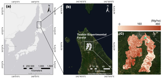
Figure 1.
Overview of our test site (a,b) and (c) the Light Detection and Ranging (LiDAR)-based above-ground biomass (AGB) map at 1.0 ha scale with 11 forest stands colored in blue.
The test site is in the hemi-boreal region, i.e., the transition between the temperate and subboreal biomes, and it covers 22,500 ha of forested area. The forest in the area consists of 90% naturally regenerated forests (approximately 36% deciduous broad-leaf forest, 20% coniferous forest, 40% mixed forest, and 4% other land types), and 10% man-made forests (conifer plantations and natural regeneration with artificial soil scarification). The dominant tree species include Abies sachalinensis (F. Schmidt) Mast., Picea jezoensis (Sieb. Et Zucc.) Carr., Picea glehnii (F. Schmidt) Mast., Quercus crispula Blume, and Betula ermanii Cham. The test site is hilly, with an elevation ranging from 13 to 580 m and a mean value of 160 m, and with a slope ranging from 0° to 56° and a mean of 17° (derived from a topography-based DTM at 10 m resolution). The annual mean temperature and annual total precipitation were 4.6 °C and 1179 mm, respectively, during the past 30 years from 1981 to 2010 [66]. The precipitation includes the snowfall, which occurred from November to April.
2.2. Three DTM Datasets
Three DTMs developed with different methodologies and spatial resolutions were used to obtain the TDX-derived forest heights (9 CHMs and 3 ModelHs); (1) LiDAR3: the airborne LiDAR-based DTM at 3 m resolution, (2) DTM10: the topography-based DTM at 10 m resolution and (3) SRTM30: the radar-based C-band SRTM DEM at 30 m resolution. We referred to each DTM with its spatial resolution at suffix (i.e., LiDAR3, DTM10 and SRTM30) in this study.
The (1) LiDAR3 was developed as a LiDAR-based DTM in the LiDAR-based AGB estimation process in 2014 (see Section 3.1). The average point density was 1.5 point/m2 [67] and it covered the entire test site. It provided the highest data precision among the three DTMs.
The (2) DTM10 was developed by the Geospatial Information Authority of Japan (GSI). It covers the entire country and has been used as the most reliable DTM nationwide. The DTM10 was generated from manually digitized contour lines with a 10 m contour interval from a 1:25,000 scale topographic map and the contour lines were drawn based on aerial photographs [68]. The standard deviation is within 5 m, and the DTM10 used in this study was downloaded from GSI homepage [69].
The SRTM DEM is the product of a joint project, the Shuttle Radar Topography Mission, of NASA, the German and Italian space agencies, and the National Geospatial-Intelligence Agency, conducted from 1999 to 2000. The SRTM employed two SARs operated at the C- and X-bands, which collected 3-D measurements of the Earth’s land surface using radar interferometry [70]. The DEM, which was developed from single pass SAR interferograms acquired in the C-band, is now freely available as the SRTM DEM with a near-global coverage. It is provided at the 30 m resolution, i.e., the 1 × 1 arc-sec (SRTM-1) and the 90 m resolution, averaging the 3 × 3 pixels (SRTM-3). The absolute vertical accuracy of the SRTM-1 is better than 9 m (90% errors) [71]. The SRTM-1 used in this study was downloaded from the U.S. Geological Survey (USGS) homepage [72] and we refer to it as (3) SRTM30.
3. Methods
3.1. AGB Estimation by Airborne LiDAR (LiDAR AGB)
The forest AGB at our test site was estimated by airborne LiDAR survey and the in-situ AGB data collected from the field survey. The LiDAR survey was conducted in 2014 by Hokkaido University and the National Institute for Environmental Studies (NIES). Its original pixel spacing was 1 m and the vertical accuracy was approximately ±15 cm [67]. The sets of point clouds classified as the first and the last echoes, i.e., the nonground and the ground echoes, were generated by a survey company [67]. The rasterized LiDAR DSM and LiDAR DTM were created from the classified echoes using the natural neighbor interpolation method (Natural Neighbor tool on Spatial Analyst of ArcGIS version 10.4.1. (Esri)) with a grid cell size of 3 m × 3 m. The LiDAR CHM was obtained by subtracting the LiDAR DTM from the LiDAR DSM.
The field measurement data conducted between 2012 and 2014 on 11 forest stands were collected from Teshio Experimental Forest. Figure 1c shows the locations of the 11 forest stands. The size of the 11 forest stands ranged from 0.1 to 0.61 ha, with the mean of 0.42 ha. In the measurements, the DBH (diameter at breast height), tree height and species were recorded for all trees with DBH > 6 cm or height > 1.3 m. The tree height was measured with an ultrasonic hypsometer (VERTEX III, Haglof, Langsele, Sweden). The AGB of each tree was estimated using the allometric equations developed for tree species in north of Hokkaido, Japan (the equation for ‘DBH (cm) as X’ in Table 2, [73]), and it was aggregated to per-hectare AGB for each stand. The per-hectare AGB of the 11 forest stands ranged from 31.8 to 317.9 Mg/ha, with the mean of 176.8 Mg/ha. We then made the polygons of the 11 forest stands, each of which contained the per-hectare AGB value generated above. The 11 forest stand polygons were geographically overlaid on the rasterized LiDAR CHM at a 3 m resolution, and the mean values of the LiDAR CHM were extracted for each of the 11 forest stand polygons. We then developed a simple regression model between the mean LiDAR CHM values and the per-hectare AGB values of the 11 forest stands, and estimated the AGB for the whole test site (hereinafter referred to as ‘LiDAR AGB’). The simple regression showed a high linear correlation between the LiDAR CHM and the per-hectare AGB (R2 = 0.86 with standard errors of 21.6 Mg/ha). The cells with negative values in the estimated LiDAR AGB were converted to zero. Figure 1c shows the LiDAR AGB map at the 1.0 ha scale. All the procedures were conducted using ArcGIS software, version 10.4.1. (Esri).
3.2. ALOS PALSAR Data Processing (HV (horizontal transmit/vertical receive) Backscatter)
We obtained five ALOS PALSAR images taken in the leaf opening period in 2010 by JAXA (Table 1). We used the 2010 PALSAR data in this study, because there was no data coverage of PALSAR (onboard the ALOS) and PALSAR-2 (onboard the ALOS-2) between 2011 and 2014 and only one PALSAR-2 image was available over our test site for 2015.

Table 1.
Details of the five Advanced Land Observing Satellite (ALOS) Phased-Array-Type L-Band Synthetic Aperture Radar (PALSAR) images used in this study.
Among the 2010 PALSAR data, we chose the data taken in the leaf opening period to keep the environment for PALSAR images as equal as possible. It is known that the radar sensors are influenced by soil moisture and tree water content, which vary depending on seasons. The penetration rate of the radar signal may also be affected by leaf fall, if the leaves are larger than the SAR-band wavelength used. In Japan, tree leaves normally emerge in the months of March to April and fall in the months of October to November, and several species in our test site, such as Quercus crispula Blume, have leaves growing larger than the ALOS L-band wavelength (23.6 cm). Therefore, we used the data taken in the leaf opening period between the months of May and October. The 2010 ALOS PALSAR data were provided at the dual polarizations of HH (horizontal transmit/horizontal receive) and HV (horizontal transmit/vertical receive), at the resolution of 12.5 m. We tested both polarizations for their correlation with the LiDAR AGB, and decided to use the HV data, as the HV imagery showed a higher correlation to the LiDAR AGB, as shown in previous studies [74,75].
The digital numbers (DN) of the five PALSAR images in HV-polarization were converted to backscattering coefficients (σ0) in units of decibel power (dB) using the Equation (1), developed for a level-1.5 product [76]:
where DN is the digital number of the PALSAR image, and the CF is the calibration factor. A value of −83.0 dB was used for CF [76]. We then overlaid the five backscattering coefficient layers in HV-polarization and took a simple arithmetic average (hereinafter referred to it as ‘HV backscatter’). The procedure was conducted using ArcGIS software, version 10.4.1. (Esri).
σ01.5 product = 10 · log10〈 DN2 〉 + CF
3.3. Development of the 12 TDX Heights
3.3.1. TDX 12 m CHMs and TDX 90 m CHMs
To obtain three TDX 12 m CHMs and three TDX 90 m CHMs, the TDX 12 m DSM data were provided by DLR [63], and the TDX 90 m DSM data were downloaded from EOC Geoservice [64]. The TDX 90 m DSM used in this study was an uncorrected DSM dataset. They were all offered in ellipsoidal heights. We first converted three DTMs (LiDAR3, DTM10 and SRTM30) to ellipsoidal heights, and then subtracted each DTM from the TDX 12 m DSM and the TDX 90 m DSM. When subtracting the DTM from the DSM, the finer resolution between the two datasets was used; the dataset in a lower resolution was resampled to the higher resolution before the subtraction. They were subsequently height-calibrated using 9 points selected from the areas with bare ground, if necessary. The cells with negative values in the resultant six CHMs were converted to zero and those above 30 m were set to null as abnormal values, as the maximum size of the trees in the site was below 30 m. All the procedures were conducted using ArcGIS software, version 10.4.1. (Esri).
The three TDX 12 m CHMs obtained were numbered and named as (1) CHM12-LiDAR3, (5) CHM12-DTM10 and (9) CHM12-SRTM30, and the three TDX 90 m CHMs obtained were also numbered and named as (2) CHM90-LiDAR3, (6) CHM90-DTM10 and (10) CHM90-SRTM30, as shown in Table 2. Table 2 shows the data numbers and names of the 9 CHMs (this Section and Section 3.3.2) and the 3 ModelHs (Section 3.3.3). Each data name consisted of two parts; the first part was to signify the type of the forest heights (CHM or ModelHs; see Introduction) followed by the spatial resolution of the DSM used (12 m, 90 m or 5 m; see ‘Datasets used as DSM’ column in Table 2). In case of ModelHs, their spatial resolution of 10 m was used. The second part was to signify the type of the DTM used (LiDAR3, DTM10 or SRTM30, see ‘Datasets used as DTM’ column in Table 2) followed by the spatial resolution of the DTM used (3 m, 10 m or 30 m; see also ‘Datasets used as DTM’ column in Table 2), and the two parts were hyphenated. The 9 CHMs and 3 ModelHs developed in Section 3.3.1, Section 3.3.2 and Section 3.3.3 were collectively called ‘12 TDX heights’ throughout this study. We also used the group name based on DTM used in the 12 TDX heights; the models using LiDAR3 for DTM (CHMs (1)–(3) and ModelH (4)) were referred to as LiDAR3 models, the models using DTM10 for DTM (CHMs (5)–(7) and ModelH (8)) were referred to as DTM10 models, and the models using SRTM30 for DTM (CHMs (9)–(11) and ModelH (12)) were referred to as SRTM30 models.
Table 2.
The list of 12 TanDEM-X (TDX) heights including 9 CHMs and 3 ModelHs. They were named based on the digital surface model (DSM) and digital terrain model (DTM) used and numbered from (1) to (12). The TDX height No. from (1) to (12) are used to identify AGB estimation models.
3.3.2. TDX 5 m CHMs
To develop the TDX 5 m CHMs, two single-pass TDX and TSX image pairs in StripMap (SM) mode were provided by DLR [63], which covered an area of approximately 30 km × 50 km. They were taken from an ascending and a descending orbit using a right-looking radar. They were both in the TDX coregistered single-look complex (CoSSC) format in HH polarization. The details are shown in Table 3. No rain was observed in the surrounding areas on the acquisition dates of the two images.
Table 3.
Details of two TDX–TSX (TerraSAR-X) image pairs used in this study.
To develop the TDX 5 m DSMs, we followed the procedure described in Avtar et al. [40]. We first performed a 2 x 2 multilooking to reduce the speckle and generated the interferogram. We then subtracted the interferometric bistatic phase simulated from each DTM (LiDAR3, DTM10 and SRTM30) and got the differential interferogram. Since the three DTMs gave the orthometric heights, the geoidal height was removed to obtain the phase corresponding to the height with reference to the WGS84 ellipsoid. The Goldstein filter [77] was applied to filter the interferometric phase, and subsequent phase unwrapping was conducted using the Minimum Cost Flow (MCF) [78] method. The unwrapped phase was combined back with the unwrapped synthetic phase of each DTM and was converted to height. Finally, we geocoded the images using the Range-Doppler approach. To obtain the TDX 5 m CHMs, we subtracted each of the three DTMs (LiDAR3, DTM10 and SRTM30) in ellipsoidal heights from the geocoded TDX 5 m DSMs. When subtracting the DTM from the DSM, the higher resolution between the two datasets was used; the dataset in the lower resolution was resampled to the higher resolution before the subtraction. They were subsequently height-calibrated using 9 points selected from the areas with bare ground. The cells with negative values in the resultant six TDX 5 m CHMs (2 TDX-TSX image pairs × 3 DTMs) were converted to zero and those above 30 m were regarded as abnormal values and set to null. The six TDX 5 m CHMs had a resolution of 5 m. The CHMs developed from the same DTM were averaged by following Equation (2) [45] to obtain the final three TDX 5 m CHMs:
where CHMmean is the mean height of the combined CHMs, CHM1 and CHM2 are the CHMs derived from the TDX-TSX image pairs # 1 and 2, and γ1 and γ2 are the corresponding coherence values.
CHMmean = (γ1 · CHM1 + γ2 · CHM2)/(γ1 + γ2)
The three TDX 5 m CHMs developed were numbered and named as (3) CHM5-LiDAR3, (7) CHM5-DTM10 and (11) CHM5-SRTM30, as shown in Table 2. The AGB estimation results derived from the three TDX 5 m CHMs were used as reference data to evaluate the AGB estimation results derived from TDX 12 m CHMs and TDX 90 m CHMs (Section 3.3.1). All the procedures were conducted using the SARscape 5.4 module of the ENVI software, version 5.4 (Esri) and ArcGIS software, version 10.4.1. (Esri).
3.3.3. ModelHs (Sinc Inversion Model-Based Forest Heights)
We used the two single-pass TDX and TSX image pairs (Table 3), the three DTMs (LiDAR3, DTM10 and SRTM30) and the Sinc inversion model to obtain three ModelHs. In the Sinc inversion model, it was assumed that the vertical backscattering profile = 1, i.e., there were equal ground and canopy backscattering coefficients. This assumption reduced the number of variables used for the forest height inversion to two, which was an effective wavenumber (kz) and coherence (γ) [79]. The key scaling factor was the local wavenumber (kz), accounting for the local angle of incidence on the sloped terrain. With the local wavenumber (kz), the height inversion reflecting the local topographical features became possible. The model details can be found in other studies [23,24,56,62,80]. The development of the ModelHs consisted of two steps: the InSAR process and the forest height (hv) calculation. First, we generated an interferogram by subtracting the flat-earth phase, followed by the coherence estimation with a window size of 10 × 12. We then geocoded coherence (γ) using each of the three DTMs with a pixel spacing of 10 m and obtained a local incidence angle (θloc) and the angle of incidence center (θ0). We then calculated the local wavenumber (kz) using Equation (3) (modified for single-pol imageries based on the equation on page 31 in [79]):
where kz is a local wavenumber, is the radar wave length in meters, θloc is the local incidence angle, is the difference in the incidence angle between the master and slave tracks, hoa is the height of ambiguity from the TDX metadata file, and θ0 is the angle of incidence center. The forest height (hv) was then estimated using coherence (γ) and local wavenumber (kz) with Equation (4) (the equation on page 34 in [79]):
where hv is the forest height, and γ is the volumetric coherence amplitude. From this process, six ModelHs (2 TDX–TSX image pairs × 3 DTMs) were obtained at the resolution of 10 m. They were subsequently height-calibrated using 9 points selected from the areas with bare ground. The cells with negative values in the resultant six ModelHs were converted to zero and those above 30 m were regarded as abnormal values and set to null. The ModelHs derived from the same DTM were then averaged by following Equation (2) to obtain the final three ModelHs. The three ModelHs obtained were numbered and named as (4) Model10-LiDAR3, (8) Model10-DTM10 and (12) Model10-SRTM30, as shown in Table 2. All the procedures were conducted using the SNAP (Sentinel Application Platform) software, version 6.0. (The European Space Agency, Paris, France), and ArcGIS software, version 10.4.1. (Esri).
hv = 2π (1 – 2 asin (|γ|0.8)/π)/kz
3.4. AGB Estimation: Non-Parametric Random Forests
A nonparametric random forest (RF) regression algorithm [81] was used to construct the AGB estimation models. In a pre-study, we tested the multiple linear regression (LM) and RF. For RF, the three RF packages of (1) randomForest in version 4.6-14 [82], (2) ranger in version 0.11.2 [83] and (3) Rborist in version 0.2-3 [84] were tested. We decided to use the (2) ranger package of RF in this study, as it gave the lowest root mean square error (RMSE) among the four models (1 LM and 3 RF models). The RMSE was calculated by Equation (5) as follows:
where Yi is the LiDAR AGB value for the cell i, and Ŷi is the estimated AGB value for the cell i, and n is the number of cells.
In RF regression, multiple regression trees are grown and merged together to obtain prediction. Each regression tree is constructed using a different sample set (a training set) from the original data. As each training set is selected randomly with replacement through bootstrap sampling, it consists of approximately two third of the entire datasets. The final result is obtained by running all the datasets down each regression tree and averaging the outputs of the entire trees. As we set the number of regression trees to the default 500, the 500 regression trees were grown using different training sets for each tree, and the final results were obtained by averaging the results of the 500 trees. In this study, the caret package was used to streamline the model building and evaluation process [85]; the package can evaluate the effect of the model-tuning parameters on performance through resampling, choose the optimal model across these parameters and estimate model performance from a training set. The predicted AGB was calculated by applying the optimal model to the entire dataset.
When growing each regression tree, one third of the datasets are not used for tree construction and remain untouched, due to sampling with replacement. These left-out samples are called the out-of-bag (OOB) samples and are used as test data to validate the model. This is the random forest cross-validation method, and in this way, there is no need to prepare test data separately. Each OOB sample is run down the tree, of which construction the OOB sample is not used, to obtain a result. This is repeated for all the OOB samples to obtain the results for each case, and the results are averaged to be used as model validation results. In the case of RF regression, the squared correlation coefficient (R2) and mean squared error (MSE) are generated using the OOB samples. In this study, the OOB-derived R2 and the relative RMSE (%) calculated from the MSE were used to evaluate the model performance and accuracies. The relative RMSE (%) was calculated by first taking the square root of the MSE and subsequently following Equation (6), as follows:
where is the arithmetic mean of the LiDAR AGB values.
3.5. Extraction of LiDAR AGB, HV Backscatter and 12 TDX Heights
To model AGB, we first created four vector layers to cover our test site with setting a cell size width and a cell size height to 50 m × 50 m (1/4 ha), 100 m × 100 m (1.0 ha), 300 m × 300 m (9.0 ha) and 500 m × 500 m (25 ha), respectively. The number of cells in each layer was 90,000 (1/4 ha), 22,500 (1.0 ha), 2500 (9.0 ha) and 900 (25 ha), respectively. We then geographically stacked the rasterized datasets of the LiDAR AGB (Mg/ha) (developed in Section 3.1), the HV backscatter (σ0) (developed in Section 3.2) and the 12 TDX heights (m) (9 CHMs and 3 ModelHs, developed in Section 3.3), and overlaid each vector layer to these stacked images. We then extracted the mean values of the stacked images for each of the 90,000 cells at 1/4 ha scale, the 22,500 cells at 1.0 ha scale, the 2500 cells at 9.0 ha scale and the 900 cells at 25 ha scale. To construct the AGB estimation models at four data scales, the mean LiDAR AGB values prescribed to each cell of the four vector layers were used as a response variable, and the mean values of the HV backscatter and the 12 TDX heights (9 CHMs and 3 ModelHs) prescribed to each cell of the same layers were used as predictors. In total, 12 AGB estimation models (× 4 scales) were constructed, and each model was identified by the TDX height No. from (1) to (12) in Table 2. These AGB estimation models were hereinafter collectively called, 12 ‘HV-TDX models’. The R2 and RMSE values of the 12 HV-TDX models were obtained from the OOB samples following the procedure in Section 3.4.
We also developed a model using the mean HV backscatter values prescribed to each cell of the four vector layers described above as a single predictor (hereinafter referred to as ‘HV model’) and models using each of the 12 mean values of the 12 TDX heights (9 CHMs and 3 ModelHs) prescribed to each cell of the same layers described above as a single predictor (hereinafter referred to as 12 ‘TDX models’), both using the mean values of the LiDAR AGB prescribed to each cell of the same layers described above as a response variable. The R2 and RMSE values of the HV model and 12 TDX models were obtained from the OOB samples following the procedure in Section 3.4 and were compared against those of the 12 HV-TDX models. To identify the 12 TDX models, the TDX height No. from (1) to (12) in Table 2 were also used.
In order to analyze the reproduction of the spatial variability by the 12 HV-TDX models, we also used SD and max values. As the OOB samples do not generate these values, we randomly chose 2/3 of the cells at each data scale as training data to develop the 12 HV-TDX models (× 4 scales) with the ranger package (Section 3.4). We used the same mean values of the LiDAR AGB, the HV backscatter and each of the 12 TDX heights prescribed to each cell of the four vector layers described above to develop the 12 HV-TDX models (× 4 scales). The developed models were applied to the remaining 1/3 of the cells (test data) at each data scale to obtain the AGB estimates. From the obtained AGB estimates, the SD and max values were derived. All the procedures and the analyses were conducted using ArcGIS software, version 10.4.1. (Esri) and R version 3.5.1 (The R Project).
In this study, the four data scales—1/4, 1.0, 9.0 and 25 ha—were used for AGB estimation and we treated the scales of 1.0 and 9.0 ha as focal scales (see Introduction and Section 5.6 for more details). We used these focal scales for further analyses, including the analyses on the TDX model (Section 4.3), the AGB retrieval at a higher AGB range (Section 4.5), the estimated AGB maps (Section 4.6), the slope-class (Section 4.8), the multiple TDX heights (Section 4.9) and the SRTM30 used as DSM (Section 4.10). We also used the 1/4 ha scale exclusively to show the estimated AGB maps in closeup (Section 4.7).
3.6. Slope-Class Analysis
It is known that topographic features have a strong effect on SAR data, because of SAR’s side-looking system [45,86]. As our test site was hilly, with slopes ranging from 0° to 56° (derived from the DTM10 at 10 m resolution), we conducted a slope-class analysis at a 1.0 ha scale for the 12 HV-TDX models to see how the varying slopes influenced the accuracy of the AGB estimation.
In this analysis, we first derived the rasterized slope data from the DTM10 (the topography-based DTM) at 10 m resolution using the Slope tool on Spatial Analyst, ArcGIS version 10.4.1. (Esri). The vector layer with the cell size of 100 m × 100 m (1.0 ha) (Section 3.5) was overlaid to the rasterized slope image to extract the mean slope values for each of the 22,500 cells. The mean slope values prescribed to each cell ranged from 0° to 40.7°. We then divided the vector layer into three sublayers based on the mean slope values prescribed to each cell; the first sublayer contained the cells with the mean slope values ranging from 0° to 9.9°, the second sublayer from 10° to 19.9°, and the third sublayer from 20° to 40.7°. The three vector sublayers had 3632, 10,499 and 8369 cells, respectively. We then followed the procedure of Section 3.5 to obtain the mean values of LiDAR AGB (Mg/ha), the HV backscatter (σ0) and the 12 TDX heights (m) (9 CHMs and 3 ModelHs) for each cell of the three sublayers, and develop the 12 HV-TDX models for each sublayer (12 HV-TDX models × 3 slope-class sublayers × 1.0 ha scale). The R2 and RMSE values of the models developed were obtained from the OOB samples following the procedure in Section 3.4. These values were used to compare the AGB estimation results among the three slope classes (0° to 9.9°, 10° to 19.9° and 20° to 40.7°). We also created new models by adding the mean slope values (°) prescribed to each cell as a new variable to the HV-TDX models and analyzed how the inclusion of the mean slope values in the initial HV-TDX models (12 HV-TDX models × 3 slope-class sublayers × 1.0 ha scale) improved the entire model performance. The models which included the slope as a variable were referred to as ‘slope models’.
3.7. Multiple TDX Heights
As we had the 12 TDX heights (9 CHMs and 3 ModelHs), we also tested a model including not one but two TDX heights to see if adding another TDX height (the 2nd TDX height) to the initial HV-TDX model was able to improve the entire model performance. This analysis was conducted at 1.0 ha scale. We refer to the TDX height in the initial HV-TDX model as the 1st TDX height. When adding the 2nd TDX height, two cases were considered; the case (i) adding the 2nd TDX height derived from the same DTM used in the 1st TDX height (e.g., CHM90-DTM10 in Table 4); the case (ii) adding the 2nd TDX height derived from the different DTM used in the 1st TDX height (e.g., CHM90-SRTM30 in Table 4).
Table 4.
Example of the multiple TDX heights analysis. In this example, either CHM90-DTM10 or CHM90-SRTM30 was added as the 2nd TDX height to the initial HV-TDX model of (5) HV + CHM12-DTM10 to derive AGB estimation results.
This analysis was to find a way to improve the AGB estimation accuracies without using the LiDAR-based DTM (LiDAR3). Therefore, the LiDAR3 models were excluded from this analysis. In total, we tested 6 pairs at the 1.0 ha scale. To develop AGB estimation models, we followed the procedure described in Section 3.5 to obtain the mean values of the LiDAR AGB (Mg/ha), the HV backscatter (σ0), the 1st TDX height (m) and the 2nd TDX height (m) for each of the 22,500 cells (100 m × 100 m vector layer). The mean values of the LiDAR AGB prescribed to each cell were used as a response variable, and the mean values of the HV backscatter and the 1st TDX heights and 2nd TDX heights prescribed to each cell were used as predictors. The R2 and RMSE values were derived from the OOB samples (Section 3.4).
4. Results
4.1. TDX Height Images
Figure 2 shows the closeup of our test site in (i) Landsat-7 ETM+ image and four TDX heights. The four TDX heights are all at 3 m resolution. In Figure 2(i), the light green color indicates grassland area, while the dark green shows forested area. In Figure 2(1)–(4), the grassland area is shown in the white color with the height of 0 m, while the forested area is shown in the black with the heights up to 30 m. The images of (1) CHM12-LiDAR3 and (3) CHM5-LiDAR3 reflect the forest height gradient from 0 to 30 m very well, while the image of (2) CHM90-LiDAR3 shows stronger color contrast in white (lower heights) and black (higher heights). The image of (4) Model10-LiDAR3 shows less black color (higher heights) than the other three images, but reflects the forest height gradient relatively well.
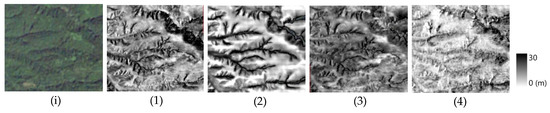
Figure 2.
The closeup of our test site in (i) pan-sharpened true color Landsat-7 ETM+ image and four TDX heights: (1) CHM12-LiDAR3, (2) CHM90-LiDAR3, (3) CHM5-LiDAR3, and (4) Model10-LiDAR3, all at 3 m resolution. The images of (1)–(4) show the spatial distribution of forest heights.
4.2. Effects of Adding 12 TDX Heights to HV Model
The data synergy effects of adding each of the 12 TDX heights to the HV backscatter were evaluated in terms of the R2 increase and the RMSE decrease over the HV model (Figure 3). In the 12 HV-TDX models, the mean LiDAR AGB values prescribed to each cell of the 1/4, 1.0, 9.0 and 25 ha scale layers (90,000, 22,500, 2500 and 900 cells, respectively) were used as a response variable and the mean values of the HV backscatter and each of the 12 TDX heights prescribed to each cell of the same layers were used as predictors to derive the R2 and RMSE values from OOB samples.
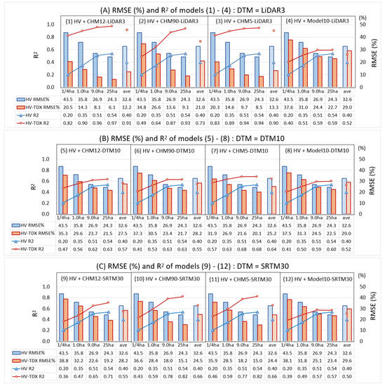
Figure 3.
The RMSE (%) and R2 of the HV model (blue) and the 12 HV-TDX models (red) shown at the 1/4, 1.0, 9.0 and 25 ha scales with the 4-scale average. The R2 and RMSE values were derived from the out-of-bag (OOB) validation results. Graphs are grouped by DTM used in the model: (A) DTM = LiDAR3, (B) DTM = DTM10 and (C) DTM = SRTM30. The HV-TDX models are numbered from (1) to (12) based on the TDX height No. (Table 2).
Compared to the HV model (Figure 3: blue line for R2 and blue bar for RMSE), all the 12 HV-TDX models yielded higher R2 (Figure 3: red line) and lower RMSE (Figure 3: red bar) across the scales. It shows a simple fact that adding any of the 12 TDX heights to the HV model improved the entire model performance. Seen by the DTM groups (LiDAR3 models, DTM10 models and SRTM30 models), the models in the same DTM group showed similar trends of R2 values; for all the DTM10 models, the R2 values leveled off at the 9.0 ha scale, while for all the SRTM30 models except the model (12), the R2 values jumped at the 9.0 ha scale; the LiDAR3 models of (1) and (3) showed almost the same R2 values across the scales.
Now, the top six models were ranked based on the average R2 values over four scales, which were in the following order: (1) HV + CHM12-LiDAR3 (R2 = 0.91) > (3) HV + CHM5-LiDAR3 (R2 = 0.90) > (2) HV + CHM90-LiDAR3 (R2 = 0.73) > (10) HV + CHM90-SRTM30 (R2 = 0.66) and (11) HV + CHM5-SRTM30 (R2 = 0.66) > (7) HV + CHM5-DTM10 (R2 = 0.64). The models (10) and (11) showed the same average R2 values. The top six models consisted of the three LiDAR3 models, two SRTM30 models and one DTM10 model. The best model (1) HV + CHM12-LiDAR3 and the 2nd best model (3) HV + CHM5-LiDAR3 both generated very high R2 > 0.82 and R2 > 0.83, respectively, across the scales. The R2 of the model (1) ranged from 0.82 to 0.97 and the largest R2 increase of the model (1) was achieved at the 1/4 ha scale from 0.20 to 0.82, or by 306%. The R2 of the model (3) ranged from 0.83 to 0.94 and the largest R2 increase of the model (3) was also achieved at the 1/4 ha scale, from 0.20 to 0.83, or by 307%. The model (1) HV + CHM12-LiDAR3 slightly outperformed the model (3) HV + CHM5-LiDAR3 which we developed for reference, indicating the high capability of the TDX 12 m DSM to yield high accuracy AGB estimates.
On the other hand, the 3rd and the two 4th best models, (2) HV + CHM90-LiDAR3, (10) HV + CHM90-SRTM30 and (11) HV + CHM5-SRTM30, started with low R2 values at the 1/4 ha scale, but at 9.0 ha the R2 jumped to 0.87, 0.78 and 0.77, respectively. Compared to the model (3) HV + CHM5-LiDAR3 which we developed for reference, the model (2) performed less well, especially at smaller scales, indicating that the TDX 90 m DSM was not able to produce AGB estimates as high an accuracy as the TDX 5 m DSM. On the other hand, the model (10) shows the R2 values almost equivalent to those of the model (11) across the scales which we developed for reference, indicating that the TDX 90 m DSM was capable of delivering AGB estimation accuracy equivalent to that of TDX 5 m DSM, when SRTM30 was used as DTM.
In contrast, the 6th best model (7) HV + CHM5-DTM10 started with an R2 of 0.57, which was higher than any other models at the 1/4 ha scale except for the LiDAR3 models of (1) and (3), but gave only a minor R2 increase afterwards; the R2 merely increased up to 0.68 at the 25 ha scale. The model (7) is a reference model for the models (5) HV + CHM12-DTM10 and (6) HV + CHM90-DTM10. This indicates that both TDX 12 m DSM and TDX 90 m DSM failed to produce AGB estimation accuracies as high as the reference model (7), when the DTM10 was used as DTM.
The bottom 3 models were the three ModelHs; (4) HV + Model10-LiDAR3, (8) HV + Model10-DTM10 and (12) HV + Model10-SRTM30. The R2 values of these 3 models were quite similar; on the average of the four scales, they were 0.52, 0.52 and 0.50, respectively. This indicates that the model performance of the 3 ModelHs were not influenced by the DTM used.
With the LiDAR AGB as a reference AGB, we also derived the SD and max values of the AGB estimates by the top 6 models over the test site, to see if the top 6 models were able to reproduce the spatial variability of the AGB properly. In this analysis, the SD and max values were used to represent the spatial variability of the AGB. First of all, by adding each of the six TDX heights (Figure 4: blue bars for SD and green bars for Max and Table 5) to the HV model (Figure 4: orange line for SD and Max and Table 5), the SD and max values became closer to those of the LiDAR AGB (Figure 4: blue line for SD and Max and Table 5) across the scales. This indicates that the six HV-TDX models better reproduced the spatial variability of the LiDAR AGB than the HV model. However, looking closer at the SD values at each scale, the SD values of all the six models except (1) and (3) were much lower than that of the LiDAR AGB, by the range of 20% to 28% at the 1/4 ha scale (Table 5). This large SD deviation of the models (2), (7), (10) and (11) from LiDAR AGB was reduced to the range of 15% to 18% at the 1.0 ha scale, to the range of 6% to 16% at the 9.0 ha scale and to the range of 0% to 12% at the 25 ha scale. This indicates that the four models reproduced SD more accurately at the larger scales, due to the reduced SD values of the LiDAR AGB at the same scales. It is also notable that the model (7) showed the SD value the closest to that of LiDAR AGB except (1) and (3) at 1/4 ha scale. On the other hand, the SD values of the models (1) and (3) were only slightly lower than those of the LiDAR AGB (8% and 7% at 1/4 ha, 4% and 4% at 1.0 ha, 2% and 4% at 9.0 ha, and 0% and 2% at 25 ha scales, for (1) and (3), respectively). The results indicate that the models (1) and (3) reproduced the spatial variability very well across the scales, while the other four models require larger scales, at least the 1.0 ha scale, to reproduce the spatial variability properly (see Section 5.6 for more details). The max values showed almost the same trend as the SD values, although the scale of the deviations were slightly larger for max values than for SD values for most models (Table 5).
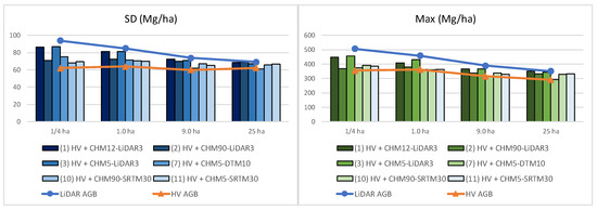
Figure 4.
The SD and max values of LiDAR AGB, HV AGB and the top six HV-TDX models at four scales from 1/4 ha to 25 ha. The SD and max values were derived from the test data.
Table 5.
The SD and max values of LiDAR AGB, HV AGB, and the top six HV-TDX models at four scales from 1/4 to 25 ha. The mark ▼ shows the decrease (%) in SD and max values from the values of LiDAR AGB. The SD and max values were derived from the test data.
4.3. Effects of Adding HV Backscatter to TDX Models
In Section 4.2, we analyzed the data synergy effects in terms of the HV model, while in this section, we analyzed them in terms of the 12 TDX models. Although the final R2 and RMSE are the same between the two cases, as the R2 values of the 12 TDX models varied from low to high, it allows us to analyze the data synergy effects in more detail. Figure 5A shows the comparison between the 3 TDX models of (1), (2) and (3) (green color) and the 3 HV-TDX models of (1), (2) and (3) (red color). The two models (1) CHM12-LiDAR3 and (3) CHM5-LiDAR3 exhibited high model performance across the scales, with R2 values of > 0.80 and > 0.79, respectively, and the model (2) CHM90-LiDAR3 showed high R2 values of > 0.87 at large scales > 9.0 ha. In these three TDX models, the effect of adding the variable of HV backscatter is minute, as they predicted AGB with very high accuracies without the HV backscatter.
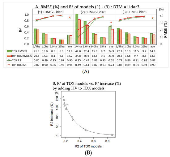
Figure 5.
(A) The RMSE (%) and R2 of the 3 TDX models (green) of (1) CHM12-LiDAR3, (2) CHM90-LiDAR3 and (3) CHM5-LiDAR3, and the 3 HV-TDX models (red) of (1) HV + CHM12-LiDAR3, (2) HV + CHM90-LiDAR3 and (3) HV + CHM5-LiDAR3, shown at 1/4, 1.0, 9.0 and 25 ha scales with the 4-scale average. The R2 and RMSE values were derived from the OOB validation results. (B) The R2 of TDX models vs. the R2 increase (%) derived from adding the HV backscatter to the TDX models. The R2 values were derived from the OOB validation results.
On the other hand, other TDX models showed low AGB estimation accuracies across the scales, with R2 values < 0.50. This indicates that those TDX models require the HV backscatter to predict AGB with high accuracy. To analyze the data synergy effects more closely, the R2 increases (%), which were derived from adding the HV backscatter to the 12 TDX models, were plotted against the R2 values of the TDX models at the 1.0 ha scale (Figure 5B). The R2 of the HV model (HV backscatter used as a single predictor) at 1.0 ha scale was 0.35. Figure 5B showed that the largest R2 increase (%) was recorded by the TDX model (4) Model10-LiDAR3 from 0.17 to 0.51 (by 209%), while the smaller R2 increase (%) was registered by (5) CHM12-DTM10 from 0.30 to 0.56 (by 85%) or by (7) CHM5-DTM10 from 0.49 to 0.63 (by 28%). It shows that the TDX models with lower R2 values had a larger R2 increase in relative terms, indicating that the data synergy effects were greater for the TDX models with lower model performance. The similar trend was also shown in the HV model (Figure 3); the HV model with lower R2 values (i.e., at 1/4 ha scale) had larger R2 increase in relative terms, when each of the 12 TDX heights was added to the HV model. Considering that the R2 increase was not linear but exponential (Figure 5B), the TDX models with low R2 values can benefit from the data synergy effects more than TDX models with high R2 values. It indicates that the data synergy approach is better used for models with low performance to improve AGB estimation accuracies.
4.4. Scale Effect Analysis
We investigated how the spatial scales influenced the AGB estimation accuracies. Figure 3 shows that both R2 and RMSE improved for all the HV-TDX models as the scale grew from 1/4 to 25 ha. In particular, the models (2), (9), (10) and (11) showed a large R2 increase and RMSE decrease at the 9.0 ha scale. The HV model (Figure 3: blue line and blue bar), which used only HV backscatter as a predictor, also showed the same trend.
We selected the model (1) HV + CHM12-LiDAR3, the best model among the 12 HV-TDX models, to further analyze the scale effects on the AGB estimation. We made AGB difference maps on a cell-by-cell basis by subtracting the AGB values estimated by the model (1) from the LiDAR AGB at four scales from 1/4 to 25 ha (Figure 6). The statistics of the resultant four AGB difference maps, including the mean, SD, the min and max values, were calculated to examine how the AGB difference between the LiDAR AGB and the AGB values estimated by the model (1) narrowed, as the data scale grew larger. The results show that as the scale grew larger, from 1/4 to 25 ha, the SD, the min and the max values of the AGB difference maps reduced. In particular, the SD values of the AGB difference maps reduced significantly at the 1.0 and 9.0 ha scale, from 24.1 (1/4 ha scale) to 16.1 Mg/ha (1.0 ha scale) and to 9.4 Mg/ha (9.0 ha scale). This indicates that the AGB values estimated by (1) became closer to the LiDAR AGB values at large scales > 9.0 ha. The AGB difference maps (Figure 6) also show that the cells with large AGB difference, which were colored in blue (AGB difference < −30 Mg/ha) and red (AGB difference > 30 Mg/ha), reduced in number significantly, both for the 9.0 and the 25 ha scales. In these maps, the cells in red indicate where the LiDAR AGB (mean values prescribed to each cell) is more than 30 Mg/ha above the AGB estimated by the model (1) at the same resolution, while the cells in blue indicate where the LiDAR AGB is more than 30 Mg/ha below the AGB estimated by the model (1) at the same resolution. The cells in white indicate that there is no difference between the LiDAR AGB and the AGB estimated by the model (1) at the same resolution.
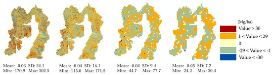
Figure 6.
The AGB difference maps between the LiDAR AGB and the predicted AGB by the best model (1) HV + CHM12-LiDAR3, shown at four scales of 1/4, 1.0, 9.0 and 25 ha. The blue color shows the AGB difference < −30 Mg/ha, while the red shows the AGB difference > 30 Mg/ha. The statistics of the mean, SD, min and max values are also shown under each map.
4.5. AGB Retrieval at Higher AGB Ranges
To analyze the AGB retrieval at higher AGB ranges, the AGB values estimated by the 12 HV-TDX models were compared against those of the LiDAR AGB at the 9.0 ha scale in a scatterplot (Figure 7). We used the 9.0 ha scale as it shows the correlation between the LiDAR AGB and the predicted AGB more clearly than the 1.0 ha scale.
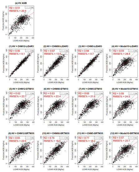
Figure 7.
LiDAR AGB vs. predicted AGB plot at the 9.0 ha scale. The R2 and RMSE values were derived from the OOB validation results. The AGB estimated by the HV model ((a) HV AGB) was also plotted against the LiDAR AGB for comparison.
The (a) HV AGB showed that the fitted curve (red line) had a large deviation from the 1 to 1 line (dashed line). In addition, the AGB values were clustered between 150 and 300 Mg/ha, and the higher AGB values > 300 Mg/ha were not retrieved. It thus showed an obvious saturation. However, by adding each of the 12 TDX heights (9 CHMs and 3 ModelHs) to the HV model (Figure 7(1)–(12)), the AGB values were distributed more evenly and the relationship between the LiDAR AGB and the estimated AGB became more linear, showing the reduced saturation issue. In particular, the three models of (1) HV + CHM12-LiDAR3, (2) HV + CHM90-LiDAR3 and (3) HV + CHM5-LiDAR3 showed very high correlations with the LiDAR AGB (R2 = 0.96, 0.87 and 0.94, respectively). The models of (10) HV + CHM90-SRTM30 and (11) HV + CHM5-SRTM30 also showed high correlations (R2 =0.78 and R2 = 0.77, respectively). On the other hand, the DTM10 models (5) to (7) and the ModelHs (4), (8) and (12) failed to retrieve higher AGB values > 300 Mg/ha, although the R2 and RMSE values improved.
4.6. Estimated TDX AGB Maps
Figure 8 and Figure 9 show the wall-to-wall maps of (A) LiDAR AGB, (B) HV AGB and the estimated AGB by the top six models with their histograms at the 1.0 ha and 9.0 ha scales, respectively. Compared to the (B) HV AGB, all the top six HV-TDX models more accurately reproduced the spatial distribution of the (A) LiDAR AGB at both scales, as the maps and the histograms showed.
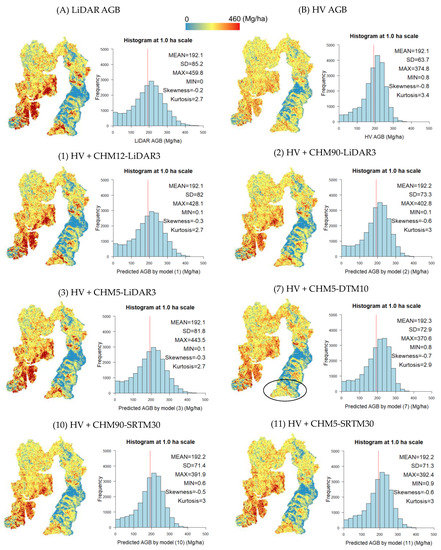
Figure 8.
The maps and the histograms of (A) LiDAR AGB, (B) HV AGB and the AGB estimated by the top six HV-TDX models of (1)–(3), (7),(10) and (11) at 1.0 ha scale. A black circle in model (7) indicates the area of large AGB deviation, compared to (A) LiDAR AGB. The mean, SD, max, min, skewness and kurtosis values are also shown on the histograms. The JGD2000 zone 12 coordinate system was used to map the AGB.
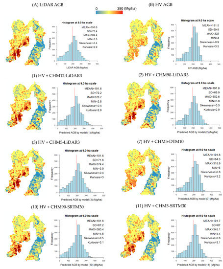
Figure 9.
The maps and the histograms of (A) LiDAR AGB, (B) HV AGB and the AGB estimated by the top six HV-TDX models of (1)–(3), (7),(10) and (11) at 9.0 ha scale. The mean, SD, max, min, skewness and kurtosis values are also shown on the histograms. The JGD2000 zone 12 coordinate system was used to map the AGB.
Focusing on the high AGB values > 300 Mg/ha at the 1.0 ha scale (Figure 8), which are shown in dark red, the five models (1) HV + CHM12-LiDAR3, (2) HV + CHM90-LiDAR3, (3) HV + CHM5-LiDAR3, (10) HV + CHM90-SRTM30 and (11) HV + CHM5-SRTM30 reproduced them well; in particular, the estimated AGB maps of (1) and (3) were almost identical to the (A) LiDAR AGB map, and so were the histograms. On the other hand, the model (7) HV + CHM5-DTM10 showed a weak reproduction of the high AGB values, and there was also the area in the south (shown in a circle) where the AGB value was much lower than the (A) LiDAR AGB. This indicates that the model (7) was unable to reproduce some of the lower AGB values < 300 Mg/ha as well. Looking at statistics, compared to the (A) LiDAR AGB, the mean values of the top six models were almost identical, but the SD, max and skewness values showed differences; especially in (B), (7), (10) and (11), the SD values were smaller than that of the (A) LiDAR AGB at the 1.0 ha scale, indicating that these models retrieved AGB in the narrower AGB ranges. At the 9.0 ha scale (Figure 9), all the models reproduced (A) LiDAR AGB values better than at the 1.0 ha scale; the statistics showed that the SD, max, skewness and kurtosis values of all the models were closer to those of the LiDAR AGB.
4.7. Closeup of Estimated TDX AGB
Figure 10 shows a closeup of the estimated AGB at the 1/4 ha scale. The high AGB values > 300 Mg/ha, which are shown in dark red, were well reproduced by (1) HV + CHM12-LiDAR3 (R2 = 0.82) and (3) HV + CHM5-LiDAR3 (R2 = 0.83), followed by (7) HV + CHM5-DTM10 (R2 = 0.57). At the 1/4 ha scale, the R2 of the model (7) was higher than (2) HV + CHM90-LiDAR3 (R2 = 0.49), (10) HV + CHM90-SRTM30 (R2 = 0.43) and (11) HV + CHM5-SRTM30 (R2 = 0.46), leading to more accurate reproduction of the spatial distribution of AGB by the model (7). The roads shown in (i) Landsat-7 ETM+ image were well reproduced in all the images in blue.
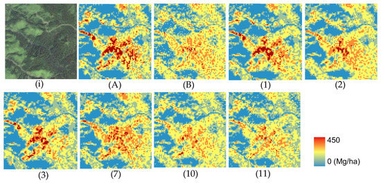
Figure 10.
The closeup of our test site in (i) pan-sharpened true color Landsat-7 ETM+ image, (A) LiDAR AGB, (B) HV AGB and the AGB estimated by the top 6 HV-TDX models of (1) HV + CHM12-LiDAR3, (2) HV + CHM90-LiDAR3, (3) HV + CHM5-LiDAR3, (7) HV + CHM5-DTM10, (10) HV + CHM90-SRTM30 and (11) HV + CHM5-SRTM30, at 1/4 ha scale.
4.8. Slope-Class Analysis
As our test site was hilly, we further analyzed how the varying slopes affected the AGB estimation accuracies. Figure 11A shows the slope map of our test site at the 1.0 ha scale by three slope classes (0° to 9.9°, 10° to 19.9°, 20° to 40.7°). It shows that the most areas with the highest slope class (20° to 40.7°, colored in blue) are located in the west, while the most areas with the lowest slope class (0° to 9.9°, colored in red) are located in the east. The areas with the second lowest slope class (10° to 19.9°, colored in yellow) are scattered around the test site. Figure 11B shows the histogram of the slope at the 1.0 ha scale, showing the mean value of 17.6° with the SD of 7.4°.
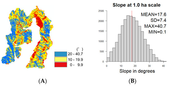
Figure 11.
(A) The slope map of our test site by three slope classes at 1.0 ha scale; the lowest slope class (0 to 9.9°) is shown in red, the second lowest slope class (10° to 19.9°) is shown in yellow, and the highest slope class (20° to 40.7°) is shown in blue. The slope map was derived from the topography-based DTM (DTM10). The number of cells of each slope class were 3632, 10,499 and 8369, respectively. (B) The histogram of the slope data in Figure 11A at 1.0 ha scale. The mean, SD, max and min values are shown on the upper right.
Table 6 shows the summary of statistics for each slope class, and the R2 values of the 12 HV-TDX models by the three slope classes. It shows that all the models produced high R2 values, ranging from 0.66 to 0.96, at the lowest slope class (0.0° to 9.9°). The three ModelHs of (4), (8) and (12), which showed the lowest R2 values in the ‘All’ class that integrated the three slope classes, also showed high R2 values at the lowest slope class (R2 ranged from 0.68 to 0.69). However, R2 values decreased as the slope moved to the higher class, and for all the models, the R2 values were the lowest at the highest slope class (20° to 40.7°); among the 12 HV-TDX models, the largest R2 decrease from the lowest to the largest slope classes was recorded by the ModelH, (12) HV + Model10-SRTM30, from 0.69 to 0.29 or by ▼59%. Other two ModelHs (4) HV + Model10-LiDAR3 and (8) HV + Model10-DTM10 also showed similarly large R2 decrease of ▼54% and ▼55%, respectively. The R2 decreases of the three ModelHs were larger than other models. This indicates that these large R2 decrease of the 3 ModelHs may have led to the low model performance of the same models at ‘All’ class. On the other hand, the two models (1) and (3) showed high R2 values across the slope classes (R2 > 0.82 and R2 > 0.83, respectively) and registered a minor R2 decrease from the lowest to the highest slope classes (▼14% for the models (1) and (3)).
Table 6.
On the left, the statistics, including the slope average, AGB average, and the number of cells for each slope class and ‘All’ class, are shown. On the right, the R2 values of the 12 HV-TDX models by the three slope classes and ‘All’ class are shown. The mark ▼ shows the R2 decrease in percent with regard to the R2 values of the lowest slope class (0°–9.9°). The row ‘All’ combines all the slope classes. The R2 values were derived from the OOB validation results.
Among the DTM10 and SRTM30 models, the model (7) HV + CHM5-DTM10 showed the highest model performance across the slope classes; the R2 ranged from 0.52 to 0.76 and the R2 decrease from the lowest to the highest slope classes was the smallest (▼31%) except for the models (1) and (3), followed by the model (10) HV + CHM90-SRTM30 (▼37%). Other DTM10 and SRTM30 models showed much larger R2 decrease, which ranged from ▼45% to ▼59%.
Table 7 shows the results of the slope models; we added the slope value (°) prescribed to each of the 22,500 cells (100 m × 100 m vector layer) as a new variable to the initial 12 HV-TDX models and derived the R2 values by slope class. The ∆R2 indicates the R2 increase from the initial 12 HV-TDX models to the slope models. The results show that the R2 increase (∆R2) ranged from 1% to 15% for the ‘All’ class, and for all the models, the R2 increase (∆R2) was the largest at the highest slope class and the smallest at the lowest slope class. The largest R2 increase of 16% was achieved at the highest slope class by the model (12) HV + Model10-SRTM30, while the lowest R2 increase of 0% was recorded by the models (1) and (3) at the lowest and the second lowest slope classes.
Table 7.
The R2 values of the slope models by three slope classes and ‘All’ class. The same slope classes of Table 6 were used. The △R2 shows the R2 increase from the initial 12 HV-TDX models to the slope models, which added the slope values as a new variable to the initial 12 HV-TDX models. The R2 values were derived from the OOB validation results.
4.9. Multiple TDX Heights
Table 8 shows the R2 increase (%) derived from adding the 2nd TDX height to the initial HV-TDX models (HV + 1st TDX height). This analysis sought to find a way to improve the AGB estimation accuracy without using LiDAR-based DTM (LiDAR3). In this analysis, the ModelHs were excluded, as their R2 values and spatial distributions of predicted AGB were almost identical to each other.
Table 8.
List of six pairs to evaluate the effects of multiple TDX heights on AGB estimation. The models designated by the capital letters (A to F) refer to case (i), in which the 2nd TDX height derived from the same DTM used in the 1st TDX height (HV-TDX model) was added to the initial HV-TDX model. The models designated by the lower-case letters (a to f) refer to case (ii), in which the 2nd TDX height derived from the different DTM used in the 1st TDX height (HV-TDX model) was added to the initial HV-TDX model. The R2 values were derived from the OOB validation results.
The R2 increase (%) was calculated from ‘R2 (1): two variables’ to ‘R2 (2): three variables’. The ‘R2 (1): two variables’ consisted of ‘HV + 1st TDX height’ and ‘HV + 2nd TDX height’. When calculating the R2 increase (%), ‘R2 (1): two variables’ with higher R2 values was used as a starting value; e.g., in the case of 1A, the R2 increase (%) was calculated from ‘HV+1st TDX height’ (R2 = 0.56) in ‘R2 (1): two variables’ to ‘HV + 1st TDX height + 2nd TDX height’ (R2 = 0.59) in ‘R2 (2): three variables’, while in case of 1a, the R2 increase (%) was calculated from ‘HV + 2nd TDX height’ (R2 = 0.59) in ‘R2 (1): two variables’ to ‘HV + 1st TDX height + 2nd TDX height’ (R2 = 0.70) in ‘R2 (2): three variables’.
The results show that, in all the pairs, case (ii) produced larger R2 increases (%) than case (i), e.g., in case of pair #1, HV + CHM12-DTM10 produced larger R2 increase (%) with the 2nd TDX height of CHM90-SRTM30 (1a: R2 increase of 18%) than with CHM90-DTM10 (1A: R2 increase of 6%). The R2 increase (%) for case (ii) ranged from 8% to 25%, with the mean of 18%, while those for case (i) ranged from 4% to 14%, with the mean of 7%. Although the pairs # 4 and 6 showed small differences between the cases (i) and (ii), the result indicates that case (ii), in which the 2nd TDX height derived from the different DTM used in the 1st TDX height was added to the initial HV-TDX model, has the possibility to improve the AGB estimation accuracy in the areas where a LiDAR-based DTM is not available.
4.10. Possibility of SRTM30 to Serve as DSM
In this section, we analyzed the possibility of SRTM30 (SRTM 30 m DEM) to serve as a DSM. We used the SRTM30 as a DTM throughout this study for the AGB estimation, which produced relatively good AGB estimation results at larger scales. However, there is still a possibility that the SRTM30 can produce better AGB estimation results if treated as a DSM.
In this attempt, we developed two CHMs using the SRTM30 as a DSM and both LiDAR3 and DTM10 as a DTM; i.e., the CHM (i): SRTM30-LiDAR3 and the CHM (ii): SRTM30-DTM10. We then developed two AGB estimation test models (A) and (B) at 1.0 ha scale using each of the two CHMs as a predictor and the LiDAR AGB of 2014 as a response variable (Table 9). In the two test models (A) and (B), we used the LiDAR AGB of 2014 (Section 3.1.) as a response variable, although the SRTM30 was the DEM product derived from the data of 2000. However, as our forest was 90% naturally regenerated forests with ages over 100 years old, the tree growth is less than 1 m3 per year [87]. Therefore, we considered the AGB growth between 2000 and 2014 was very small. The 100 m × 100 m (1.0 ha) vector layer described in Section 3.5 was used to extract the mean values of the LiDAR AGB and the two CHMs for each of the 22,500 cells (100 m × 100 m vector layer). No HV backscattering data were used for this analysis. The R2 and RMSE values of each test model were derived from the OOB samples by following the procedure described in Section 3.4.
Table 9.
The list of a response variable and predictors used for two AGB estimation test models (A) and (B). Predictor (i) was derived from SRTM30 as DSM and LiDAR3 as DTM, and predictor (ii) was derived from SRTM30 as DSM and DTM10 as DTM.
Firstly, the results of the test model (A), which used the CHM (i) SRTM30-LiDAR3 as a predictor, were compared against those of the LiDAR3 models from (1) to (4) in Table 10, and next, the results of the test model (B), which used the CHM (ii) SRTM30-DTM10 as a predictor, were compared against those of DTM10 models from (5) to (8) also in Table 10, and finally, the results of the test models (A) and (B) were compared against the SRTM30 models from (9) to (12) in Table 10, which were derived using the SRTM30 as DTM (see Materials and Methods). The models from (1) to (12), which we used as reference here, were derived without HV backscattering data following the procedure described in the TDX model of Section 3.5.
Table 10.
R2 and RMSE values of two AGB estimation test models (A) and (B), in which the CHMs (i) and (ii) were used as a predictor, respectively, and LiDAR AGB as a response variable for both models. The R2 and RMSE values of the 12 TDX models, which were derived with LiDAR AGB as a response variable and each of 12 TDX heights as a predictor (see Section 3.5), are also shown. All the R2 and RMSE values were derived from the OOB validation results.
Table 10 shows that, compared to the LiDAR3 models (1)–(4), the performance of the test model (A) (R2 = 0.14, RMSE = 41.1%) was close to that of the model (4) HV + Model10-LiDAR3 (R2 = 0.17, RMSE = 41.6%), but much lower than other three LiDAR3 models. On the other hand, compared to the DTM10 models (5)–(8), the test model (B) showed much lower R2 and higher RMSE values (R2 = −0.07, RMSE = 45.8%). Lastly, compared to the SRTM30 models (9)–(12), the R2 and RMSE values of the test model (A) were slightly worse than those of the SRTM30 models, while the R2 and RMSE values of the test model (B) were much worse than the SRTM30 models. The results showed that the model (A) had a possibility to produce reasonable AGB estimation results, but the model (B) had no possibility. This is fatal, because in a large-scale AGB estimation, it is inevitable to use the DTM10 (the topography-based DTM) to obtain CHM, as it is the only DTM prepared nationwide in Japan.
The analysis showed that all the 12 TDX models served well as forest vertical information to estimate AGB in our test site than the CHMs (i) and (ii). This indicates the possibility that the penetration of C-band SAR signal of the SRTM30 through the canopy is deep in our test site, leading to the scattering phase center of the SRTM30 too low to serve as a DSM. In Ni et al. [30], the penetration depth was derived by subtracting the ALOS InSAR height from the canopy top height derived from the ASTER GDEM, and used the penetration depth as forest vertical information to predict AGB. Although the ALOS InSAR height is not a DTM, but the scattering phase center of the ALOS PALSAR data is well below the canopy top due to the long wavelength of the PALSAR, creating the penetration depth which served as forest vertical information to predict AGB well. In our case, the SRTM30 is not completely a DTM either, but the scattering phase center of the SRTM30 is also low below the canopy top in our test site with medium forest cover. By subtracting the SRTM30 (C-band) from the TDX DSM (X-band), it was also able to produce the penetration depth, which may have served as forest vertical information and predicted AGB well in our test site. It is difficult to determine if the SRTM30 should be used as DTM based on these results only, but it was inferred that in our test site, the models which used SRTM30 as a DTM were capable of producing better AGB predictions overall, rather than using it as a DSM.
5. Discussion
5.1. High AGB Estimation Accuracies of LiDAR3 Models
The results of our study showed that adding each of the 12 TDX heights (nine CHMs and three ModelHs) to the HV backscatter improved the R2 values in all the models, regardless of the forest height creation method (either the CHMs or ModelHs), the spatial scales or the types of DSMs and DTMs used. This means that the data synergy approach worked well in this study. The size of the model improvement, however, depended most strongly on the forest height creation method (either the CHMs or ModelHs), shown by the fact that, compared to the models using nine CHMs, all the three ModelHs yielded much lower AGB estimation accuracies across the scales (Figure 3). Although the slope-class analysis showed that the three ModelHs produced high R2 values (0.68 to 0.69 at 1.0 ha scale) for the lowest slope class, their R2 values were still lower than those of the nine CHMs (Table 6) (for more details on AGB estimation accuracies of ModelHs, see Section 5.4). The size of the model improvement subsequently depended on both the DSMs and DTMs used in the models; it was shown that for models using a high-accuracy DTM, i.e., LiDAR3, the accuracy of the DSMs influenced the AGB estimation results a lot, as shown by the fact that among the three LiDAR3 models of (1), (2) and (3), two models (1) and (3), which were derived from the high-resolution DSMs of TDX 12 m DSM and TDX 5 m DSM, respectively, produced high R2, while the model (2), which was derived from the low-resolution DSM of TDX 90 m DSM, yielded much lower R2 at smaller scales < 1.0 ha. On the contrary, for models using a low-accuracy DTM, i.e., DTM10 and SRTM30, the accuracy of the DTMs (DTM10 and SRTM30) have stronger influence than the DSMs on the AGB estimation results, as shown by the fact that among the three SRTM30 models of (9), (10) and (11), very similar R2 and RMSE values were obtained across the scales, even though the high-resolution DSMs were used for the models (9) and (11). It explains why the two models of (10) and (11) were both ranked as the top six models with the same average R2 value.
Among the 12 HV-TDX models, R2 increase was the largest in two LiDAR3 models of (1) HV + CHM12-LiDAR3 and (3) HV + CHM5-LiDAR3. Previous studies have also shown that a CHM obtained from InSAR data and an ALS-derived DTM retrieved forest properties well [51,52]. Our three LiDAR3 models, (1), (2) and (3), retrieved higher AGB values > 300 Mg/ha effectively. In previous studies, Saatchi et al. [88] estimated AGB in the tropical forest of Costa Rica with an elevation ranging from 35 to 135 m a.s.l., and showed that by adding the InSAR height to the fully polarized backscatter coefficients that were both derived from AIRSAR, an RMSE was reduced from 25.0% to 20.3% at the 1/4 ha scale and from 28.3% to 17.1% at the 1.0 ha scale (the related RMSE values (%) were calculated by us based on the RMSE values and the mean AGB values in the paper [88]). Zhang et al. [89] also estimated AGB in a transition forest between the boreal and temperate biomes in the U.S. with a topography of flat to gently rolling with a maximum elevation change of < 135 m, and reported that the combined use of the fully polarized L-band Uninhabited Aerial Vehicle SAR (UAVSAR) backscatter and a canopy height made from the stereo-imagery of the Panchromatic Remote Sensing Instrument for Stereo Mapping (PRISM) on-board the ALOS reduced the RMSE from 37.0% to 28.2% at the 1/4 ha scale and from 27.0% to 20.2% at the 1.0 ha scale. Both studies used the ALS-based DTM for height development. In our case, the combined use of the HV backscatter and the forest height derived from TDX 12 m DSM and LiDAR DTM ((1) HV + CHM12-LiDAR3) reduced the RMSE from 43.5% to 20.5% at the 1/4 ha scale and from 35.8% to 14.3% at the 1.0 ha scale, and also, the combined use of the HV backscatter and the forest height derived from TDX 5 m DSM and LiDAR DTM ((3) HV + CHM5-LiDAR3) reduced the RMSE from 43.5% to 20.3% at the 1/4 ha scale and from 35.8% to 14.6% at the 1.0 ha scale. Compared to the previous studies [88,89], the RMSE of our models (1) and (3) were very close to and lower than those of Saatchi et al. [88] at the 1/4 and 1.0 ha scales, respectively, and much lower than those of Zhang et al. [89] at both scales. Additionally, the combined use of the HV backscatter and the forest height derived from TDX 90 m DSM and LiDAR DTM ((2) HV + CHM90-LiDAR3) reduced the RMSE from 43.5% to 34.8% at the 1/4 ha scale and from 35.8% to 26.6% at the 1.0 ha scale, which were approximately 6% higher than those of Zhang et al. [89]. Considering that the previous studies [88,89] employed airborne datasets for either one or both of the variables and full polarimetry data (HH, HV and VV) for the SAR backscatter, our models (1) to (3), which used spaceborne datasets for both variables and single-polarization HV data for the SAR backscatter, performed very well.
The three TDX models (1) CHM12-LiDAR3, (2) CHM90-LiDAR3 and (3) CHM5-LiDAR3 also showed high model performance without the variable of HV backscatter at all the scales for (1) and (3) and at large scales > 9.0 ha for (2). The TDX models of (1) CHM12-LiDAR3 and (3) CHM5-LiDAR3 achieved the RMSE of 15.0% and 16.3% at the 1.0 ha scale, respectively. In earlier studies, Solberg et al. [43] analyzed the accuracy of the AGB estimated from the TDX InSAR heights and the ALS-based DTM in Norway, and reported an RMSE of 19% at the stand level (the stand size being 1.0 to 2.9 ha); in addition, Rahlf et al. [45] analyzed the accuracy of the forest volume estimated from the TDX InSAR heights and the ALS-based DTM also in Norway with hilly terrain with altitudes ranging from 50 to 650 m a.s.l., showing an RMSE of 18.1% at stand level (the stand size being 1.0 to 3.0 ha). Compared to these studies, our models of (1) and (3) achieved lower RMSE values, although a smaller cell size was used in our study. In Yu et al. [44], five different remote sensing datasets (ALS, TDX InSAR, TSX SAR radargrammetry, World-View2 and aerial stereo imagery) were compared for their ability to predict forest attributes including the forest AGB in a boreal forest in Finland. They found that the RMSE of the TDX InSAR-derived AGB predictions was 20.69% (the plot size of 32 m × 32 m). As their study area was located in a flat area (elev. 125 m to 185 m) with the forest consisting of 75% conifers, we also used the RMSE of the predicted AGB at the lowest slope class of 0° to 9.9° for comparison; the RMSE of our two models (1) CHM12-LiDAR3 and (3) CHM5-LiDAR3 at the lowest slope class (0° to 9.9°) and at the 1/4 ha scale were 16.6% and 17.1%, respectively. Although the previous study used a smaller plot size than ours, the results showed that our models of (1) and (3) worked very well, considering that our test site was located in a hemi-boreal forest with mixed forest structures (36% broadleaf, 20% conifer and 40% mixed forest).
These results show that the (1) HV + CHM12-LiDAR3 and (3) HV + CHM5-LiDAR3 models generated highly accurate AGB estimation results, outperforming not only other models in our study, but also the models of the previous studies. The slope-class analysis also showed that the models (1) and (3) yielded high R2 values across the slope classes. In addition, both models reproduced the spatial variability of the LiDAR AGB very well across the scales, and predicted AGB without the variable of HV backscatter, with an accuracy as high as the corresponding HV-TDX models. These analyses verified that in our test site in the hemi-boreal region, the TDX 12 m DSM had a high capability to estimate AGB with very high accuracy in the form of CHM with the LiDAR-based DTM (LiDAR3) across the scales and the slope classes. As for the (2) HV + CHM90-LiDAR3 model, high model performance, which was very close to those of the models (1) and (3), was achieved at large scales > 9.0 ha, both with and without the variable of HV backscatter. The slope-class analysis also showed that the model (2) yielded high model performance at the lowest slope class < 10°, even at the 1.0 ha scale. It indicates that the TDX 90 m DSM was also able to yield high AGB estimation accuracies in the form of CHM with the LiDAR-based DTM (LiDAR3) at large scales > 9.0 ha and also at the 1.0 ha scale for flat terrains.
One thing we need to mention here is a possibility that the LiDAR3 models performed well because our LiDAR AGB, which was used as a response variable in the 12 HV-TDX models, was also derived from the LiDAR DTM (LiDAR3) and LiDAR DSM. However, the accuracy of LiDAR data is normally very high, reflecting the surface features correctly. Therefore, we consider this effect to be minor. However, as LiDAR data is not necessarily available in most countries, the LiDAR3 model results may be used as reference data to evaluate the AGB estimation results derived from non-LiDAR-based DTMs, e.g., SRTM30 and DTM10 in our case, to find the optimal models among them (see Section 5.2 and Section 5.3).
5.2. High Usability of TDX 90 m CHM and Multiple TDX Heights
Among the models using DTM10 and SRTM30, the two best models were (10) HV + CHM90-SRTM30 and (11) HV + CHM5-SRTM30. They delivered high model performance at large scales > 9.0 ha (R2 = 0.78 and 0.82 for (10) and R2 = 0.77 and 0.82 for (11) at 9.0 and 25 ha, respectively), which were only slightly lower than those of the LiDAR3 model, (2) HV + CHM90-LiDAR3 (R2 = 0.87 and 0.93 at 9.0 and 25 ha, respectively). The models (10) and (11) also reproduced the SD values well at large scales > 9.0 ha (Table 5 and Figure 9). This finding verifies that the TDX 90 m DSM was able to generate high AGB estimation accuracies at large scales > 9.0 ha not only with LiDAR3, but also with SRTM30. Considering that the TDX 12 m DSM did not show any good AGB estimation results, either with DTM10 or SRTM30 across the scales, and that (10) HV + CHM90-SRTM30 achieved almost the same model performance as (11) HV + CHM5-SRTM30, which we developed for reference, the model (10) HV + CHM90-SRTM30 has high potential for producing accurate AGB estimations at large scales in the areas where LiDAR-based DTM is not available. As the datasets of TDX 90 m DSM and SRTM 30 m DEM (SRTM30) are freely available worldwide, the model (10) is highly useful for large-scale AGB estimation in the hemi-boreal forest. In addition, the slope-class analysis showed that, on the areas with low slopes below 10°, the model (10) can provide higher AGB estimation accuracies, even at the 1.0 ha scale, indicating that this model has a possibility to produce high AGB estimation accuracies at 1.0 ha scale, if applied to flat terrains.
One previous study that used SRTM30 as the DTM for AGB estimation was that of Sadeghia et al. [49], which estimated the AGB in forests north of Quebec City, Canada, using 14 variables, including the CHM derived from the TDX InSAR DSM and the height-calibrated SRTM30 as a DTM. They used a random forest regression algorithm and obtained an R2 of 0.62 and an RMSE of 34% at the stand level (0.5 ha to 4 ha). The RMSE of our model (10) HV + CHM90-SRTM30 was 28.4% at the 1.0 ha scale and we did not add calibration to the SRTM30. As the parameters used in the previous study and ours were considerably different and could not be compared directly, but considering that the previous study employed 14 variables and used a larger stand size, our model (10) yielded very good results.
Additionally, it has been demonstrated in our study (Table 8) that the use of two TDX heights derived from two different DTMs has a possibility to improve the model performance further at the 1.0 ha scale. Taking up the model (10), for example, by adding the 2nd TDX height of CHM12-DTM10 to (10) HV + CHM90-SRTM30 model, R2 increased from 0.59 to 0.70 and the RMSE decreased from 28.4% to 24.3% at the 1.0 ha scale. This large model improvement may be because the spatial distribution of heights of DTM10 and SRTM30 differed somewhat from each other, which allowed the 2nd TDX height to serve as a new parameter and improve the entire model performance. This shows the possibility of using multiple forest heights in non-LiDAR3 models to improve AGB estimation accuracies at the 1.0 ha scale.
5.3. Low AGB Estimation Accuracies of DTM10 Models and Height Deviations
Among the DTM10 models, the best model was (7) HV + CHM5-DTM10. Motohka et al. [90] used the CHMs developed from the five ALOS PRISM DSMs and DTM10 (the same topography-based DTM as used in this study) to estimate the AGB at the 1/4 ha scale. The study area of this previous study was geographically very close to ours. The previous study showed that RMSE ranged from 22.1% to 32.6% at the 1/4 ha scale, while that of our model (7) CHM5-DTM10 (without the HV backscatter) was 36.1% at the same scale. The RMSE of our model (7) was higher than that of the previous study. One possible reason for this is that we used the LiDAR data covering varied terrains from flat to hilly for AGB estimation, leading to a higher RMSE than the previous study, which studied plot-based AGB estimates. Another possible reason, which is also related to the wide area coverage of the LiDAR data, is a height deviation of DTM10 from LiDAR3 in some parts of our test site. The details are described below.
The DTM10 models of (5), (6) and (7) showed a considerably lower model performance at all scales, except for the 1/4 ha, than the other HV-TDX models. Compared by the accuracy of the DTM datasets, however, the DTM10 has better data accuracy of ±5 m [69] than SRTM30, and therefore, the DTM10 models should have yielded higher AGB estimation accuracies than the SRTM30 models. To determine a possible cause, we compared the LiDAR AGB and the AGB estimated by (7) HV + CHM5-DTM10 model. Figure 12a is a AGB difference map on a cell-by-cell basis obtained by subtracting the AGB estimated by the model (7) from the LiDAR AGB at the 9.0 ha scale, and Figure 12b is a height difference map on a cell-by-cell basis obtained by subtracting the DTM10 from LiDAR3 at the same scale. We examined if there were any areas of unusual AGB and height difference. In Figure 12a, the areas with AGB difference > 30 Mg/ha are shown in red, which correspond well to the areas of the height difference < −5 m in Figure 12b. This large AGB deviation was also shown in Figure 8(7). We also drew an AGB difference map between the LiDAR AGB and the AGB estimated by (10) HV + CHM90-SRTM30 model, the best model among the SRTM30 models (Figure 12c), and a height difference map between the LiDAR3 and SRTM30 (Figure 12d) for comparison. Figure 12c,d showed no signs of unusual AGB or height differences in a particular area, although the heights of SRTM30 are higher than those of LiDAR3 by approximately 3 to 4 m across the test site (Figure 12d).
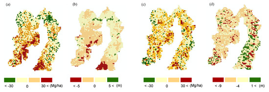
Figure 12.
The AGB difference map (a) between LiDAR AGB and the estimated AGB by (7) HV + CHM5-DTM10 model, the height difference map (b) between LiDAR3 and DTM10, the AGB difference map (c) between the LiDAR AGB and the estimated AGB by (10) HV + CHM90-SRTM30 model, and the height difference map (d) between LiDAR3 and SRTM30, all at the 9.0 ha scale.
We removed the cells with height difference < −5 m in Figure 12b, and derived the AGB estimations again for the three DTM10 models of (5) HV + CHM12-DTM10, (6) HV + CHM90-DTM10, and (7) HV + CHM5-DTM10. The R2 values increased from 0.62 to 0.71 for (5), 0.63 to 0.71 for (6), and 0.68 to 0.76 for (7) at the 9.0 ha scale. We repeated the procedure at the 1.0 ha scale; the R2 increased from 0.56 to 0.66 for (5), from 0.53 to 0.60 for (6) and from 0.63 to 0.73 for (7). Non-DTM10 models did not show any large model improvement at either the 1.0 or 9.0 ha scale. The analysis showed that the performance of the DTM10 models can be improved by 18% and by 15% at the most at the 1.0 and 9.0 ha scales, respectively, indicating that the DTM10 models have the potential to outperform the SRTM30 models at the 1.0 ha scale. All the R2 values used here were derived from the OOB validation results.
It was confirmed that the height deviation of DTM10 from LiDAR3 in some parts of our test site led to the low AGB estimation accuracies of the DTM10 models. The areas of the height deviation were located in relatively high AGB areas on the high slopes. In the study of Motohka et al. [90], there were also the AGB estimation errors in high mountainous regions. They ascribed this to the errors in the DSM or DTM in regions of steep topography. The DTM10 was made from contour lines based on aerial photographs (AP). In the case of AP, it is known that the solar elevation during image acquisition influences the accuracy of heights [91], while the SRTM30 was developed from SAR data, which is also strongly influenced by the slope and aspect because of its side-looking system [86]. There is a possibility that the radar has an advantage over the AP for elevation measurements in forests with not dense but moderate canopy cover, like at our test site. On the other hand, the fact that both the LiDAR3 and SRTM30 employed pulse-based systems may have produced the consistency in the height distributions between the LiDAR3 and SRTM30. This indicates the possibility that the LiDAR3 and SRTM30, not DTM10, have height errors.
To further analyze the underlying cause for the deviation of DTM10 from LiDAR3, we examined the height difference between LiDAR3 and DTM10 on a cell-by-cell basis in terms of slope and aspect. We used the factors of slope and aspect in this analysis, as the results of our study and a previous study [90] showed large AGB estimation errors in regions of steep topography, and also the AP technique which was used to develop DTM10 can be negatively influenced by shadows when solar elevation is low [91].
We first derived the slope and aspect from the topography-based DTM (DTM10) at 10 m resolution using the Slope and Aspect tools on the Spatial Analysis of ArcGIS software, 10.4.1. (Esri). The aspect data obtained in degrees from 0 (due north) to 360 (again due north) was categorized into eight classes with numbers from 1 to 8; the number 1 for east, 2 for southeast, 3 for south, 4 for southwest, 5 for west, 6 for northwest, 7 for north and 8 for northeast. The three cells with the value −1, which showed a flat area, were removed. The vector layer with the cell size of 100 m × 100 m (1.0 ha scale) described in Section 3.5 was used to extract the mean slope and the majority aspect values for each of the 22,500 cells (the 100 m × 100 m vector layer). We obtained the mean slope values ranging from 0° to 40.7° and the aspect values ranging from 1 to 8. The slope vector layer was then divided into seven slope sublayers by 5° (Table 11) and the aspect vector layer was then divided into eight aspect sublayers by aspect (Table 12). Through this process, we obtained the seven slope sublayers with each cell containing its own slope value (°), and the eight aspect sublayers with each cell containing aspect values from 1 to 8. Each vector sublayer was used to extract the mean height difference between LiDAR3 and DTM10 for each cell.
Table 11.
The statistics of height difference between LiDAR3 and DTM10 by slope class by 5°, with slope average, AGB average and the number of cells, and the mean, SD, min and max values of the height difference.
Table 12.
The statistics of height difference between LiDAR3 and DTM10 by aspect, with slope average, AGB average and the number of cells, and the mean, SD, min and max values of the height difference. The three cells with a value -1, which indicated a flat area, were removed.
Table 11 shows the summary of statistics regarding the height difference by the seven slope classes. It shows that the SD, min and max values increased gradually as the slope moved up to the higher class, although the mean values were not so different; e.g., the SD values increased from 2.8 (the lowest slope class; 0°–4.9°) to 5.1 (the highest slope class; 30°–40.7°), and the min and max values also increased from –8.9 and 9.3 (the lowest slope class; 0°–4.9°) to -16.1 and 13.5 (the highest slope class; 30°–40.7°), respectively. This indicates that the magnitude of the height deviations was larger at higher slope classes.
Table 12 shows the summary of height difference by the eight aspect classes. It shows that the values of the mean height difference were negative for the cells facing east, southeast, south, southwest and west, meaning that the LiDAR3 is lower than DTM10 in those cells, while the values of the height difference were positive in the cells facing northwest, north and northeast, indicating that the LiDAR3 is higher than DTM10 in those cells.
It is difficult to determine the cause from this analysis only, but it indicates that the height deviations between LiDAR3 and DTM10 have some relation to slope and aspect. Considering that the cells with particular aspects have the particular mean height tendencies (the negative or positive mean values), it may be related to the tilt of the airborne LiDAR system itself. There is also a possibility that it is related to the shadow effects. A previous study [91] showed that in the case of the AP analysis, the probability of measuring the correct terrain surface decreased in shadows, due to the reduced spectral signatures and image dynamics. Further studies on the slope, aspect and other possible factors are necessary to specify the cause of these height deviations, because the DTM10 is indispensable for a country-level AGB estimation, especially at smaller scales.
5.4. Low AGB Estimation Accuracies of ModelHs
The three ModelHs had the lowest model performance among the 12 HV-TDX models across the scales. This result showed that, regarding the AGB estimations in our test site, the forest height creation method of the CHM (subtracting a DTM from a DSM) worked better than the ModelH (the Sinc inversion model-based approach). However, it was also shown that at the lowest slope class (0° to 9.9°), the three ModelHs were able to produce high AGB estimation accuracies (R2 = 0.68 to 0.69) at the 1.0 ha scale (Table 6). This indicates that this Sinc inversion model-based methodology may be better suited for flat terrains.
In a previous study, Askne et al. [58] used 18 TDX InSAR pairs (VV-pol) and the RVoG model to estimate the AGB for 201 forest stands (the stand size being 1.0 to 12.0 ha) and reported that the RMSE varied between 17% and 40%. This previous study used a test site which was fairly flat, with elevations ranging from 120 to 145 m a.s.l. To compare the AGB estimation results of our three ModelHs against those of Askne et al. [58], we used the RMSE values at the lowest slope class; the RMSE of our three ModelHs, of (4) Model10-LiDAR3, (8) Model10-DTM10 and (12) Model10-SRTM30 (without the variable of HV backscatter), at the lowest slope class at the 1.0 ha scale ranged from 38.0% to 40.3%. Another previous study by Soja et al. [80], which used a two-level model inversion scheme and single-pass TDX InSAR data (VV-pol) for AGB estimation, showed that the RMSE ranged from 12% to 19% at a plot level (32 circular 40-m radius plots). Soja et al. [80] also used the same test site as Askne et al. [58], but added another test site with a strongly undulating topography with ground slopes on stand level up to 19°. For comparison against the AGB estimation accuracies of Soja et al. [80], we used the RMSE of ‘All’ class of the three models, which ranged from 39.5% to 40.5% at the 1.0 ha scale. Both previous studies used ALS-based DTMs to derive InSAR data. Considering that Askne et al. [58] used a larger stand size (1.0 to 12.0 ha) than ours (1.0 ha), the RMSE of our three ModelHs were well within the RMSE range of Askne et al. [58], but were much higher than those of Soja et al. [80]. The high RMSE values of the ModelHs may be attributed to other factors. We used single-pass TDX InSAR data, as used in these two previous studies [58,80], but in HH polarization, due to the data unavailability. It is known that the HH data have a stronger contribution from the ground than the VV data [92], which has a high possibility of affecting the accuracy of the developed ModelHs and lowering the model performance. Additionally, in the Sinc inversion model, it is assumed that the ground and canopy backscatter coefficients are equal. According to Soja et al. [80], this assumption is not well applied to dense forests or forests with multilayer structures. The forest at our test site is neither dense nor uniform, but mixed. It is possible that this Sinc inversion model did not work well in our forest structure. Further studies in the areas available with VV-pol data and with similar forest structures to ours are required for more appropriate analysis of the Sinc inversion model.
5.5. Slope-Class Analysis
The slope-class analysis showed that all the 12 HV-TDX models yielded high R2 values (0.66 to 0.96) at the lowest slope class (0° to 9.9°), indicating the possibility for them to yield high-accuracy AGB estimations in a flat area. Among the DTM10 and SRTM30 models, the model (7) HV + CHM5-DTM10 showed the highest R2 values across three slope classes at the 1.0 ha scale (Table 6), and the smallest R2 decrease of −31% from the lowest to the highest slope classes. Considering that other DTM10 models, (5) HV + CHM12-DTM10, (6) HV + CHM90-DTM10 and (8) HV + Model10-DTM10, showed much lower R2 and larger R2 decrease, the model (7) performed very well. The models (5) and (6) were derived from the TDX 12 m DSM and TDX 90 m DSM respectively, which were developed using multiple TDX images [37]. However, they showed a lower model performance across the slope classes than the model (7), which was derived from the DSM we developed from two TDX–TSX image pairs for reference (Table 3). This may be because the TDX-TSX image pairs we chose were better suited for the DSM creation, as we chose the images carefully based on the parameters, including coherence, height of ambiguity, baseline information and precipitation. We need to analyze the cause for the low R2 values of the models (5) and (6)—e.g., slope, forest type and climatic factors—to find a suitable environment for the models derived from these TDX DSM products, as the number of AGB estimation applications using these TDX DSM products is expected to increase in the future. In addition, considering that all the models performed well at the lowest slope class and that the model performance decreased as the slope got higher, the accuracies of the datasets used in the models, including the HV backscatter, three DSMs and three DTMs, might be strongly influenced by slope in the data production process. This analysis showed that the topographic features including slope should be carefully taken into consideration in AGB estimation, especially when using SAR data in a hilly terrain.
In the slope models in which a variable slope was added to the initial HV-TDX models, we found that the R2 increase was largest at the highest slope class (20° to 40.7°). Rahlf et al. [45] used four different remote sensing datasets, including the ALS, stereo aerial photogrammetry, InSAR and radagrammetry, to retrieve AGB with a stand size of 1 to 3 ha. The stands were located in southern Norway with slopes ranging from 1° to 30°, with the mean of 9°. They incorporated the parameters of slope and aspect in the models derived from the four different remote sensing datasets, and found that the InSAR data were affected the most by topography among the four, but RMSE decrease derived from incorporating slope and aspect to the InSAR model were less than 1%. They ascribed this to the data generation method; they combined ascending and descending TDX imageries to generate a DSM, which moderated the effects of slope and aspect. They used an ALS-derived DTM for InSAR data development. We also derived an RMSE decrease by adding the slope variable to the TDX model (3) CHM5-LiDAR3 at 1.0 ha scale and the RMSE decrease was 5%. We cannot directly compare our results to those of this previous study, as we only used the slope as an additional parameter. However, the RMSE decrease was larger for our slope model (3) CHM5-LiDAR3 + Slope, although we also combined the ascending and descending TDX images to generate the TDX 5 m DSM. This larger RMSE decrease may be because our test site covers varied terrains, from flat to hilly, with the slope ranging from 0° to 56° (calculated from the DTM10 at 10 m resolution). Considering that the terrain of the previous study was less hilly than ours and it was shown in our study that R2 increases derived by adding slope variable to the HV-TDX models were largest at the highest slope class, our complex terrain may have led to the slightly larger model improvement by the slope model (3) CHM5-LiDAR3 + Slope. It showed the necessity of incorporating the parameter of topographic features in AGB estimation models in hilly terrains.
5.6. Suitable Scales for AGB Estimation
In our study, increasing spatial scales have led to the improved performance of all the HV-TDX models. This scale effect is also shown in other studies; Zhang et al. [89] estimated AGB using UAVSAR backscatter and ALOS PRISM height and showed that the accuracy of AGB estimation was higher, when a 1.0-ha plot size, rather than a 1/4-ha plot size, was used; Saatchi et al. [88] also predicted AGB using AIRSAR data and reported better AGB estimation results at the 1.0 ha scale, compared to 1/4 or 1/2 ha scales.
When using the spatial data derived from satellites or airborne platforms for AGB estimation, however, it is important not only to improve the AGB estimation accuracy but also to reproduce the spatial variability of forest AGB appropriately, as this information is inevitable for timber production, disaster management and ecosystem service evaluation, including CO2 monitoring. According to Saatchi et al. [88], in the case of SAR data, the spatial variability of forest structures is maintained well in datasets at higher resolutions, as radar sensors with a high performance capture them. However, the high-performance sensors also produce errors associated with the datasets such as radar speckle noise and the orthorectification errors involved in data stacking [88,89], which leads to decreased AGB estimation accuracy. Up-scaling reduces these errors and the spatial variability of forest structure and biomass, and improves the AGB estimation accuracy. At the same time, however, up-scaling homogenizes the spatial variability to some extent. In our study, all the 12 HV-TDX models yielded a better model performance as the scales grew larger, from 1/4 to 25 ha (Figure 3), but the SD values of the LiDAR AGB (a reference AGB) also reduced from 93.9 Mg/ha at 1/4 ha to 69.0 Mg/ha at 25 ha scale (Table 5: validation results on test data) and so did the predicted AGB of the six models (Table 5: validation results on test data). The reduced SD indicates the poor reproduction of the spatial variability. Therefore, it is important to keep the balance between maintaining the spatial variability for spatial analysis of the forest AGB and improving the AGB estimation accuracies for correct AGB monitoring, and to find a suitable scale to achieve this balance.
To find a suitable scale for AGB estimation, we firstly analyzed the SD values of the LiDAR AGB and secondly considered the size of the AGB change that needs to be monitored. Firstly, we analyzed the SD change in the LiDAR AGB from the scales of 3 (the original LiDAR AGB data size) to 500 m (25 ha scale) (Figure 13 and Table 13). To derive the SD, max, mean, min, skewness and kurtosis values (statistical values) of the LiDAR AGB at nine scales from 3 to 500 m, we first created eight vector layers (except the 3 m scale) at the scales shown in Table 13 (for 50, 100, 300 and 500 m, we used the same vector layers described in Section 3.5). The eight vector layers were overlaid on the rasterized LiDAR AGB data at 3 m resolution to extract the mean LiDAR AGB values for each cell at each vector scale, from which the statistical values were derived. The statistical values were also derived from the LiDAR AGB data at the original 3 m resolution. The procedure details are also described in Section 3.5.
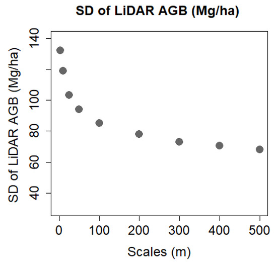
Figure 13.
The shift in SD values of the LiDAR AGB at scales from 3 (the original LiDAR AGB data resolution) to 500 m (25 ha).
Table 13.
The values of SD, max, mean, min, skewness and kurtosis of the LiDAR AGB at scales from 3 (the original LiDAR AGB data resolution) to 500 m (25 ha). The mark ▼ shows the decrease (%) in SD and max values from the corresponding values of LiDAR AGB in 3 m resolution. The decrease (%) was not calculated for mean, min, skewness and kurtosis values, as they are observable from the values.
Figure 13 and Table 13 show that the large SD decrease (−10% to −12%) occurred at small scales below 25 m, followed by a moderate SD decrease (−7%) at medium scales between 50 and 100 m and by a slight SD decrease (−2% to −5%) at large scales above 200 m. By up-scaling the original LiDAR AGB data at the 3 m scale to 25 m, approximately one fourth of the SD decrease (-22%) occurred (Table 13). The reduction of the SD values became stable at the medium scales of 50 m (1/4 ha) and 100 m (1.0 ha). The stability of the SD values is inevitable to achieve high AGB estimation accuracy. Saatchi et al. [88] estimated AGB at the tropical forest of Costa Rica using plot sizes of 1/4, 1/2 and 1.0 ha. Their analysis showed that the large variability of forest structure and biomass started to be more stable at plot sizes > 1/4 ha, and they determined the 1.0 ha scale as a suitable scale for estimating AGB in the area, as the distribution of the AGB at 1.0 ha scale does not deviate strongly from normality or stationarity (mean and variance do not vary significantly in space). As indicators for the normality, the symmetric probability distribution and small skewness and kurtosis were used. In our case, the skewness values of the LiDAR AGB were close to 0 at all the scales, but the kurtosis values were below 2.5 at scales below 50 m (the kurtosis value of 3.0 represents a normal distribution), indicating that the LiDAR AGB has a low degree of peakedness for the scales below 50 m and that it deviates from the normal distribution. In addition, the histograms of the LiDAR AGB at the scales below 50 m did not show symmetric probability distributions either. Considering that the SD values were stabilized at scales > 50 m (1/4 ha) and the LiDAR AGB values were normally distributed at scales > 100 m (1.0 ha), the minimum scale for AGB estimation should also be 100 m (1.0 ha) in our case.
Secondly, we considered a suitable AGB estimation scale from the standpoint of the size of AGB change that needs to be monitored. The AGB change occurs from several causes which also vary in scale, e.g., tree logging for timber production, a natural disaster and deforestation for construction. In our test site, the 1/4 ha scale should reflect the in-situ AGB the most among the four data scales, as the plot size of our field survey ranged from 0.1 to 0.61 ha, with the mean of 0.42 ha. However, in practice, timber production activities, such as clear-cutting and thinning, are carried out at scales larger than 1/4 ha, considering the economic efficiency of the activities. In Japan, a clear cutting up to 20 ha is allowed for each logging case in a standard practice [93], and the average size of forest stands, the minimum unit for forest management, ranges from 2.6 to 12.9 ha in Hokkaido prefecture, depending on the forest ownership (private, prefectural and national forests) in the years from 2014 to 2016. Given the average size of the forest stands and the forest management practice, estimating AGB at the 1.0 ha scale is suitable for monitoring the AGB change caused by timber production. A large-scale AGB change also occurs as a result of natural disasters and deforestation by construction. In recent years, typhoons with an increased intensity have hit Japan more frequently, which topple trees across several tens of hectares, and also, the construction of forestry roads has been partially promoted for timber production in Japan and the deforestation spans several hundreds of hectares. In these cases, estimating AGB at 9.0 ha will suffice to monitor the AGB change. On top of that, AGB estimation accuracy significantly improves at the 9.0 ha scale (Figure 3), and a high AGB estimation accuracy is achievable by using the datasets of not only higher resolutions but also lower ones which are freely available worldwide (e.g., TDX 90 m DSM and SRTM 30 m DEM). Although up-scaling the original LiDAR AGB data at a 3 m resolution to the 9.0 ha scale reduces the spatial variability by 45%, the availability of the global data and its high AGB estimation accuracy have a high potential to contribute to the large-scale AGB monitoring and disaster management.
With all the analyses combined, the 1.0 ha scale is suitable for monitoring a local-scale AGB change caused by e.g., timber production, while the 9.0 ha scale is appropriate for monitoring a large-scale AGB change caused by e.g., natural disaster and human-induced large-scale deforestation in our test site. Focusing on the AGB estimation accuracies and the reproduction of SD values at 1.0 ha and 9.0 ha scales (Figure 3 and Figure 4), the models (1), (2) and (3) performed very well; the two models of (1) and (3) can be used for AGB monitoring at both scales, and the model (2) can be used at 9.0 ha scale, when the LiDAR-based DTM is available. On the other hand, two models of (10) and (11) performed very well at large scales > 9.0 ha; these models are better suited to estimating AGB at the 9.0 ha scale, in the areas where LiDAR-based DTM is not available. However, our analysis also showed the possible ways to improve the AGB estimation accuracies at the 1.0 ha scale for the models using non-LiDAR-based DTMs including (10) and (11); to focus on the flat terrains with slopes < 10° (see Section 4.8) and to use two TDX heights derived from two different DTMs (see Section 4.9). These measures may also be considered when models derived from non-LiDAR-based DTMs are used for AGB estimation. There is also a future possibility that DTM10 models produce higher AGB estimation accuracies at both scales, if the DTM10 deviations from the LiDAR3 are adequately fixed.
5.7. Future Analysis for Time Series
In this study, we used five ALOS PALSAR images taken during the leaf opening period from May to October, and two pairs of TDX–TSX images taken in September, by carefully choosing the datasets based on the factors including coherence, baseline information, precipitation and seasons (see Section 3.2 and Section 3.3). However, to properly monitor the AGB change, it is also important to consider if the methodology developed in this study can be applied to a different time period and is capable of producing the AGB estimation with the same accuracy as shown in this study.
It is known that a SAR satellite has a strong sensitivity to moisture and therefore, SAR images taken during a rainy season or in areas with high soil moisture tend to be affected due to varied dielectric constant. Pulliainen et al. [94] used InSAR coherence observations of 14 C-band SAR image pairs to retrieve stem volume in Finland. They used both the snow-free summertime and snow-covered wintertime images taken under various weather conditions. They showed that in multiple stem-volume retrieval attempts, each using the SAR images taken under heavy precipitation, strong wind, low temperature and melting snow, the level of coherence of all the attempts became low, resulting in a low correlation to stem volume. The same holds true for SAR backscatter and AGB. Lucas et al. [95] showed that for the ALOS PALSAR data acquired during wet period, increases in σ0f were most significant at L-band HH (σ0f: units of topographically normalized backscattering intensities) and they observed that the data acquired during minimal surface moisture and rainfall allowed better estimation of AGB over Queensland, Australia.
In Japan, the wet season normally starts in September and ends in November. There is a high possibly that the reduced SAR sensitivity to AGB caused by high levels of moisture would produce less accurate AGB estimation results in the rainy season. However, focusing on our test site, which is located in the north of Hokkaido, the place does not suffer from heavy rain during the wet season, but snow falls heavily in winter. It was also shown by Pulliainen et al. [94] that the snow-covered terrain works positively for SAR sensitivity to forest AGB; the snow-covered winter images are superior to images obtained under summer conditions, yielding the highest stem volume retrieval performance, as the interferometric images obtained under snow-covered conditions show very high coherence values. There is a high possibility that our AGB estimation method can be applied to a dry winter time. Although a seasonal AGB change between summer and winter may be difficult to detect, because the tree growth between the two seasons is minor in our study forest, but it clearly enhances the opportunity to monitor AGB in two seasons over the years, which helps to better understand the forest AGB change in the hemi-boreal region.
6. Conclusions
In this study, we compared the accuracies of AGB values estimated by integrating the PALSAR backscatter and each of the 12 TDX heights at four scales from 1/4 to 25 ha in the hemi-boreal forest in Japan. The 12 TDX heights developed in this study included the nine CHMs and the three ModelHs; the nine CHMs were derived from the three DSMs of the TDX 12 m DSM, TDX 90 m DSM and TDX 5 m DSM that we developed from two TDX–TSX image pairs for reference, and the three DTMs of an airborne LiDAR-based DTM, a topography-based DTM and the SRTM 30 m DEM; the three ModelHs were developed from the two TDX–TSX image pairs and the three DTMs with the Sinc inversion model. The major findings were as follows: (i) the combined use of the HV backscatter and each of the 12 TDX heights improved the R2 and RMSE values of all the models, showing that the data synergy approach worked well in this study; (ii) the TDX 12 m DSM had a high capability to estimate AGB with very high accuracy in the form of CHM, but the use of the LiDAR-based DTM was required; (iii) the TDX 90 m DSM was able to achieve high AGB estimation accuracies not only with the LiDAR-based DTM but with SRTM DEM in the form of CHM, but it was limited to large scales > 9.0 ha; (iv) the ModelHs performed less well than the CHMs, and the ModelHs were more suitable for AGB estimation in flat terrains where they produced high AGB estimation accuracy; (v) all the models achieved higher model performance at the lowest slope class below 10°, showing that the slope is one of the largest factors to influence the AGB estimation results; (vi) the multiple forest heights derived from two different DTMs had a potential for improving AGB estimation accuracies of the models derived from non-LiDAR-based DTM at 1.0 ha scale; and (vii) SRTM 30 m DEM (SRTM30) showed a high possibility to serve as a DTM in the hemi-boreal forest in AGB estimation. These findings clarified the strengths and the limitations of the 12 HV-TDX heights, and more attention needs to be paid not only to the spatial resolutions of datasets and the data creation methods, but also to the topographic features of the area to produce AGB estimation with higher accuracy.
With a global AGB mapping becoming an imminent task, we found that the TDX 90 m DSM and SRTM 30 m DEM (as DTM), which are both freely available worldwide, have a high potential to contribute to it at large scales of > 9.0 ha and even at the 1.0 ha scale using multiple forest heights or focusing on flat terrains. On the other hand, regional or national deforestation management requires AGB mapping at even smaller scales, and the TDX 12 m DSM and a nationwide DTM should play a major role in this. However, we also found that there was height deviations between a topography-based DTM (DTM10) available in Japan and the LiDAR-based DTM in some areas of our test site. Removing the areas of the height deviations increased the AGB estimation accuracies by 18% at the 1.0 ha scale. It indicates that the TDX 12 m DSM and DTM10 could yield better AGB estimation results, if the height deviations were adequately fixed. For future deforestation management, the verification of the data accuracy of DTM10 and LiDAR-based DTM are urgently needed.
Author Contributions
A.H. processed the LiDAR data, L-band SAR data and TanDEM-X InSAR data, carried out the research and wrote the paper draft. K.T. was responsible for the field measurements and assisted in developing the methodology and improving the paper draft. R.A. corresponded for the TDX data acquisition, instructed the InSAR data processing and assisted in methodology development. T.T. provided the scientific guidance for L-band SAR data processing and assisted in conceptualization of the study. F.N. supervised the entire research and assisted in conceptualization of the study. All authors have read and agreed to the published version of the manuscript.
Funding
The LiDAR survey used in this study was financially supported by the Grants-in-Aid for Scientific Research (KAKENHI no 26292076) from the Ministry of Education, Culture, Sports, Science and Technology, Japan.
Acknowledgments
The authors would like to express sincere gratitude to four anonymous reviewers for their valuable comments and suggestions to improve the manuscript. The authors also greatly appreciate the DLR for providing the TanDEM-X data and the JAXA for providing L-band SAR data, and are also very thankful to Masato Hayashi of JAXA for his scientific comments on this research, and Lei Zhao of Chinese Academy of Forestry for his help on Sinc inversion methodology.
Conflicts of Interest
The authors declare no conflict of interest.
References
- The Intergovernmental Panel on Climate Change (IPCC). Available online: https://www.ipcc.ch/reports/ (accessed on 30 September 2019).
- Myneni, R.B.; Dong, J.; Tucker, C.J.; Kaufmann, R.K.; Kauppi, P.E.; Liski, J.; Zhou, L.; Alexeyev, V.; Hughes, M.K. A large carbon sink in the woody biomass of Northern forests. Proc. Natl. Acad. Sci. USA 2001, 98, 14784–14789. [Google Scholar] [CrossRef] [PubMed]
- Houghton, R.A. Aboveground forest biomass and the global carbon balance. Glob. Chang. Biol. 2005, 11, 945–958. [Google Scholar] [CrossRef]
- Dittmann, S.; Thiessen, E.; Hartung, E. Applicability of different non-invasive methods for tree mass estimation: A review. For. Ecol. Manag. 2017, 398, 208–215. [Google Scholar] [CrossRef]
- Zaki, N.A.M.; Latif, Z.A. Carbon sinks and tropical forest biomass estimation: A review on role of remote sensing in aboveground-biomass modelling. Geocarto Int. 2017, 32, 701–716. [Google Scholar] [CrossRef]
- Sinha, S.; Jeganathan, C.; Sharma, L.K.; Nathawat, M.S. A review of radar remote sensing for biomass estimation. Int. J. Environ. Sci. Technol. 2015, 12, 1779–1792. [Google Scholar] [CrossRef]
- Rodríguez-Veiga, P.; Wheeler, J.; Louis, V.; Tansey, K.; Balzter, H. Quantifying Forest Biomass Carbon Stocks from Space. Curr. For. Rep. 2017, 3, 1–18. [Google Scholar] [CrossRef]
- Kaasalainen, S.; Holopainen, M.; Karjalainen, M.; Vastaranta, M.; Kankare, V.; Karila, K.; Osmanoglu, B. Combining Lidar and Synthetic Aperture Radar Data to Estimate Forest Biomass: Status and Prospects. Forests 2015, 6, 252–270. [Google Scholar] [CrossRef]
- Le Toan, T.; Beaudoin, A.; Riom, J.; Guyon, D. Relating Forest Biomass to SAR Data. IEEE Trans. Geosci. Remote Sens. 1992, 30, 403–411. [Google Scholar] [CrossRef]
- Luckman, A.; Baker, J.R.; Kuplich, T.M.; Yanasse, C.C.F.; Frery, A.C. A study of the relationship between radar backscatter and regenerating forest biomass for space borne SAR instrument. Remote Sens. Environ. 1997, 60, 1–13. [Google Scholar] [CrossRef]
- E-SAR. The Experimental Airborne SAR System of DLR. Available online: https://www.dlr.de/hr/en/Portaldata/32/Resources/dokumente/institut/E_SAR_data_sheet.pdf (accessed on 30 November 2019).
- Imhoff, M.L.; Johnson, P.; Holford, W.; Hyer, J.; May, L.; Lawrence, W.; Harcombe, P. BioSAR (TM): An inexpensive airborne VHF multiband SAR system for vegetation biomass measurement. IEEE Trans. Geosci. Remote Sens. 2000, 38, 1458–1462. [Google Scholar] [CrossRef]
- Dubois-Fernandez, P.C.; Toan, T.L.; Daniel, S.; Oriot, H.; Chave, J.; Blanc, L.; Villard, L.; Davidson, M.W.J.; Petit, M. The TropiSAR Airborne Campaign in French Guiana: Objectives, Description, and Observed Temporal Behavior of the Backscatter Signal. IEEE Trans. Geosci. Remote Sens. 2011, 50, 3228–3241. [Google Scholar] [CrossRef]
- Uninhabited Aerial Vehicle Synthetic Aperture Radar, Jet Propulsion Laboratory (JPL), California Institute of Technology. Available online: https://www.jpl.nasa.gov/missions/uninhabited-aerial-vehicle-synthetic-aperture-radar-uavsar/ (accessed on 30 September 2019).
- Sun, G.; Ranson, K.J.; Guo, Z.; Zhang, Z.; Montesano, P.; Kimes, D. Forest biomass mapping from lidar and radar synergies. Remote Sens. Environ. 2011, 115, 2906–2916. [Google Scholar] [CrossRef]
- Tian, X.; Su, Z.; Chen, E.; Li, Z.; Tol, C.; Guo, J.; He, Q. Estimation of forest above-ground biomass using multi-parameter remote sensing data over a cold and arid area. Int. J. Appl. Earth Obs. Geoinf. 2012, 14, 160–168. [Google Scholar] [CrossRef]
- Avtar, R.; Suzuki, R.; Sawada, H. Natural forest biomass estimation based on plantation information using PALSAR data. PLoS ONE 2014, 9, e86121. [Google Scholar] [CrossRef] [PubMed]
- Avtar, R.; Suzuki, R.; Takeuchi, W.; Sawada, H. PALSAR 50 m mosaic based national level biomass estimation for REDD+ policies implementation. PLoS ONE 2013, 8, e74807. [Google Scholar] [CrossRef]
- Wang, Y.; Davis, F.W.; Melack, J.M.; Kasischke, E.S.; Christensen, N.L. The effects of changes in forest biomass on radar backscatter from tree canopies. Int. J. Remote Sens. 1995, 16, 503–513. [Google Scholar] [CrossRef]
- Imhoff, M.L. Radar backscatter and biomass saturation: Ramifications for global biomass inventory. IEEE Trans. Geosci. Remote Sens. 1995, 33, 511–518. [Google Scholar] [CrossRef]
- Bamler, R.; Hartl, P. Synthetic aperture radar interferometry. Inverse Probl. 1998, 14, R1. [Google Scholar] [CrossRef]
- Ferretti, A.; Prati, C.; Rocca, F. Permanent scatterers in SAR interferometry. IEEE Trans. Geosci. Remote Sens. 2001, 39, 8–20. [Google Scholar] [CrossRef]
- Cloude, S.R.; Papathanassiou, K.P. Polarimetric SAR interferometry. IEEE Trans. Geosci. Remote Sens. 1998, 36, 1551–1565. [Google Scholar] [CrossRef]
- Krieger, G.; Papathanassiou, K.P.; Cloude, S.R. Spaceborne polarimetric SAR interferometry: Performance analysis and mission concepts. EURASIP J. Appl. Signal Process. 2005, 20, 3272–3292. [Google Scholar] [CrossRef]
- Persson, H.; Fransson, J.E.S. Forest Variable Estimation Using Radargrammetric Processing of TerraSAR-X Images in Boreal Forests. Remote Sens. 2014, 6, 2084–2107. [Google Scholar] [CrossRef]
- Solberg, S.; Riegler, G.; Nonin, P. Estimating Forest Biomass from TerraSAR-X Stripmap Radargrammetry. IEEE Trans. Geosci. Remote Sens. 2015, 53, 154–161. [Google Scholar] [CrossRef]
- Vastaranta, M.; Holopainen, M.; Karjalainen, M.; Kankare, V.; Hyyppa, J.; Kaasalainen, S. TerraSAR-X Stereo Radargrammetry and Airborne Scanning LiDAR Height Metrics in Imputation of Forest Aboveground Biomass and Stem Volume. IEEE Trans. Geosci. Remote Sens. 2014, 52, 1197–1204. [Google Scholar] [CrossRef]
- Toutin, T.; Gray, L. State-of-the-art of elevation extraction from satellite SAR data. ISPRS J. Photogramm. Remote Sens. 2000, 55, 13–33. [Google Scholar] [CrossRef]
- U.S. Geological Survey (USGS) HP. Available online: https://www.usgs.gov/centers/ca-water-ls/science/interferometric-synthetic-aperture-radar-insar?qt-science_center_objects=0#qt-science_center_objects (accessed on 22 December 2019).
- Ni, W.; Zhang, Z.; Sun, G.; Guo, Z.; He, Y. The Penetration Depth Derived from the Synthesis of ALOS/PALSAR InSAR Data and ASTER GDEM for the Mapping of Forest Biomass. Remote Sens. 2014, 6, 7303–7319. [Google Scholar] [CrossRef]
- Fayad, I.; Baghdadi, N.; Bailly, J.S.; Barbier, N.; Gond, V.; Hérault, B.; Hajj, M.E.; Fabre, F.; Perrin, J. Regional Scale Rain-Forest Height Mapping Using Regression-Kriging of Spaceborne and Airborne LiDAR Data: Application on French Guiana. Remote Sens. 2016, 8, 240. [Google Scholar] [CrossRef]
- Hudak, A.T.; Lefsky, M.A.; Cohen, W.B.; Berterretche, M. Integration of lidar and Landsat ETM+ data for estimating and mapping forest canopy height. Remote Sens. Environ. 2002, 82, 397–416. [Google Scholar] [CrossRef]
- Vastaranta, M.; Wulder, M.A.; White, J.C.; Pekkarinen, A.; Tuominen, S.; Ginzler, C.; Kankare, V.; Holopainen, M.; Hyyppa, J.; Hyyppa, H. Airborne laser scanning and digital stereo imagery measures of forest structure: Comparative results and implications to forest mapping and inventory update. Can. J. Remote Sens. 2013, 39, 382–395. [Google Scholar] [CrossRef]
- Krieger, G.; Moreira, A.; Fiedler, H.; Hajnsek, I.; Eineder, M.; Zink, M. TanDEM-X: A satellite formation for high resolution SAR interferometry. IEEE Trans. Geosci. Remote Sens. 2007, 45, 3317–3341. [Google Scholar] [CrossRef]
- Rodriguez-Cassola, M.; Prats, P.; Schulze, D.; Tous-Roman, N.; Steinbrecher, U.; Marotti, L.; Nannini, M.; Younis, M.; L’opez-Dekker, P.; Zink, M.; et al. First Bistatic Spaceborne SAR Experiments with TanDEM-X. IEEE Geosci. Remote Sens. Lett. 2012, 9, 33–37. [Google Scholar] [CrossRef]
- Zink, D.; Bachmann, M.; Bräutigam, B.; Fritz, T.; Hajnsek, I.; Krieger, G.; Moreira, A.; Wessel, B. TanDEM-X: The new global DEM takes shape Article. IEEE Trans. Geosci. Remote Sens. 2014, 2, 8–23. [Google Scholar] [CrossRef]
- Wessel, B. TanDEM-X Ground Segment–DEM Products Specification Document, Public Document TD-GS-PS-0021. 2018, 3.1.; EOC, DLR: Weßling, Germany, 2018. [Google Scholar]
- AIRBUS Defence and Space. Available online: https://www.intelligence-airbusds.com/elevation-models/ (accessed on 30 September 2019).
- Grohmann, C.H. Evaluation of TanDEM-X DEMs on selected Brazilian sites: Comparison with SRTM, ASTER GDEM and ALOS AW3D30. Remote Sens. Environ. 2018, 212, 121–133. [Google Scholar] [CrossRef]
- Avtar, R.; Yunus, A.P.; Kraines, S.; Yamamuro, M. Evaluation of DEM generation based on Interferometric SAR using TanDEM-X data in Tokyo. Phys. Chem. Earth 2015, 83, 166–177. [Google Scholar] [CrossRef]
- Zhang, K.Q.; Gann, D.; Ross, M.; Robertson, Q.; Sarmiento, J.; Santana, S.; Rhome, J.; Fritz, C. Accuracy assessment of ASTER, SRTM, ALOS, and TDX DEMs for Hispaniola and implications for mapping vulnerability to coastal flooding. Remote Sens. Environment 2019, 225, 290–306. [Google Scholar]
- Karila, K.; Vastaranta, M.; Karjalainen, M.; Kaasalainen, S. Tandem-X interferometry in the prediction of forest inventory attributes in managed boreal forests. Remote Sens. Environ. 2015, 159, 259–268. [Google Scholar] [CrossRef]
- Solberg, S.; Astrup, R.; Breidenbach, J.; Nilsen, B.; Weydahl, D. Monitoring spruce volume and biomass with InSAR data from TanDEM-X. Remote Sens. Environ. 2013, 139, 60–67. [Google Scholar] [CrossRef]
- Yu, X.; Hyyppa, J.; Karjalainen, M.; Nurminen, K.; Karila, K.; Vastaranta, M.; Katoh, M. Comparison of laser and stereo optical, SAR and InSAR point clouds from air- and space-borne sources in the retrieval of forest inventory attributes. Remote Sens. 2015, 7, 15933–15954. [Google Scholar] [CrossRef]
- Rahlf, J.; Breidenbach, J.; Solberg, S.; Næsset, E.; Astrup, R. Comparison of four types of 3D data for timber volume estimation. Remote Sens. Environ. 2014, 155, 325–333. [Google Scholar] [CrossRef]
- Treuhaft, R.; Lei, Y.; Gonçalves, F.; Keller, M.; dos Santos, J.R.; Neumann, M.; Almeida, A. Tropical-forest structure and biomass dynamics from TanDEM-X radar interferometry. Forests 2017, 8, 277. [Google Scholar] [CrossRef]
- Santos, J.R.; de Jesus Silva, C.V.; Galvão, L.S.; Treuhaft, R.; Mura, J.C.; Madsen, S.; Gonçalves, F.G.; Keller, M.M. Determining Aboveground Biomass of the Forest Successional Chronosequence in a Test-Site of Brazilian Amazon through X- and L-Band Data Analysis. In Proceedings of SPIE; Hadjimitsis, D.G., Themistocleous, K., Michaelides, S., Papadavid, G., Eds.; SPIE: Bellingham, WA, USA, 2014; Volume 9229, p. 92291. [Google Scholar]
- Walker, W.S.; Kellndorfer, J.M.; Pierce, L.E. Quality of SRTM C-and X-band interferometric data: Implications for the retrieval of vegetation canopy height. Remote Sens. Environ. 2007, 106, 428–448. [Google Scholar] [CrossRef]
- Sadeghia, Y.; St-Ongeb, B.; Leblonc, B.; Prieurd, J.F.; Simarde, M. Mapping boreal forest biomass from a SRTM and TanDEM-X based on canopy height model and Landsat spectral indices. Int. J. Appl. Earth Obs. Geoinf. 2018, 68, 202–213. [Google Scholar] [CrossRef]
- Simard, M.; Zhang, K.; Rivera-Monroy, V.H.; Ross, M.S.; Ruiz, P.L.; Castaneda-Moya, E.; Twilley, R.R.; Rodriguez, E. Mapping Height and Biomass of Mangrove Forests in Everglades National Park with SRTM Elevation Data. Photogramm. Eng. Remote Sens. 2006, 72, 299–311. [Google Scholar] [CrossRef]
- Bispo, P.D.; Pardini, M.; Papathanassiou, K.P.; Kugler, F.; Balzter, H.; Rains, D.; Dos Santos, J.R.; Rizaev, I.G.; Tansey, K.; Dos Santos, M.N.; et al. Mapping forest successional stages in the Brazilian Amazon using forest heights derived from TanDEM-X SAR interferometry. Remote Sens. Environ. 2019, 232, 111194. [Google Scholar] [CrossRef]
- Sadeghi, Y.; St-Onge, B.; Leblon, B.; Simard, M. Canopy Height Model (CHM) Derived from a TanDEM-X InSAR DSM and an Airborne Lidar DTM in Boreal Forest. IEEE J. Sel. Top. Appl. Earth Obs. 2016, 9, 381–397. [Google Scholar] [CrossRef]
- Cloude, S.R. Polarisation: Applications in Remote Sensing, 1st ed.; Oxford University Press: Oxford, UK, 2010. [Google Scholar]
- Papathanassiou, K.P.; Cloude, S.R. Single-baseline polarimetric SAR interferometry. IEEE Trans. Geosci. Remote Sens. 2001, 39, 2352–2363. [Google Scholar] [CrossRef]
- Cloude, S.R.; Papathanassiou, K. Three-stage inversion process for Polarimetric SAR interferometry. IEE Proc. Radar Sonar Navig. 2003, 150, 125–134. [Google Scholar] [CrossRef]
- Olesk, A.; Praks, J.; Antropov, O.; Zalite, K.; Arumäe, T.; Voormansik, K. Interferometric SAR Coherence Models for Characterization of Hemiboreal Forests Using TanDEM-X Data. Remote Sens. 2016, 8, 700. [Google Scholar] [CrossRef]
- Askne, J.I.H.; Santoro, M.; Smith, G.; Fransson, J.E.S. Multitemporal repeat-pass SAR interferometry of boreal forests. IEEE Trans. Geosci. Remote Sens. 2003, 41, 1540–1550. [Google Scholar] [CrossRef]
- Askne, J.I.H.; Fransson, J.E.S.; Santoro, M.; Soja, M.J.; Ulander, L.M.H. Model-based biomass estimation of a hemi-boreal forest from multitemporal TanDEM-X acquisitions. Remote Sens. 2013, 5, 5574–5597. [Google Scholar] [CrossRef]
- Askne, J.I.H.; Soja, M.J.; Ulander, L.M.H. Biomass estimation in a boreal forest from TanDEM-X data, lidar DTM, and the interferometric water cloud model. Remote Sens. Environ. 2017, 196, 265–278. [Google Scholar] [CrossRef]
- Chen, E.X.; Li, Z.Y.; Cloude, S.R.; Papathanassiou, K.P.; Pottier, E. Comparison of Methods to Derive Forest Height from Polarimetric SAR Interferometry. In Proceedings of the Dragon 1 Programme Final Results 2004–2007, Beijing, China, 21–25 April 2008; ESA: Paris, France, 2008. [Google Scholar]
- Soja, M.J.; Persson, H.; Ulander, L.M.H. Estimation of Forest Height and Canopy Density from a Single InSAR Correlation Coefficient. IEEE Trans. Geosci. Remote Sens. Lett. 2015, 12, 646–650. [Google Scholar] [CrossRef]
- Chen, H.; Cloude, S.R.; Goodenough, D.G. Forest Canopy Height Estimation Using Tandem-X Coherence Data. IEEE J. Sel. Top. Appl. Earth Obs. Remote Sens. 2016, 9, 3177–3188. [Google Scholar] [CrossRef]
- The German Aerospace Centre (DLR). Available online: https://www.dlr.de/EN/Home/home_node.html (accessed on 30 September 2019).
- The EOC Geoservice of the Earth Observation Center (EOC) of the German Aerospace Center (DLR). Available online: https://geoservice.dlr.de/web/dataguide/tdm90/ (accessed on 30 September 2019).
- Japan Long Term Ecological Research Network (JaLTER). Available online: http://www.jalter.org/ (accessed on 30 September 2019).
- National Land Information Division, National Spatial Planning and Regional Policy Bureau, MLIT of Japan. Available online: http://nlftp.mlit.go.jp/ksj/index.html (accessed on 30 September 2019).
- Hokkai Kousoku. LiDAR Survey in Teshio Experimental Forest, Technical Report; Hokkaido University: Sapporo, Japan, 2016. [Google Scholar]
- Ardiansyah, P.O.D.; Yokoyama, R. DEM generation method from contour lines based on the steepest slope segment chain and a monotone interpolation function. ISPRS J Photogramm. Remote Sens. 2002, 57, 86–101. [Google Scholar] [CrossRef]
- Geospatial Information Authority of Japan (GSI). Available online: https://fgd.gsi.go.jp/download/menu.php (accessed on 30 September 2019).
- U.S. Releases Enhanced Shuttle Land Elevation Data, Jet Propulsion Laboratory (JPL), California Institute of Technology. Available online: https://www.jpl.nasa.gov/news/news.php?release=2014-321 (accessed on 30 September 2019).
- Farr, T.G.; Rosen, P.A.; Caro, E.; Crippen, R.; Duren, R.; Hensley, S.; Kobrick, M.; Paller, M.; Rodriguez, E.; Roth, L.; et al. The shuttle radar topography mission. Rev. Geophys. 2007, 45, 1–33. [Google Scholar] [CrossRef]
- U.S. Geological Survey (USGS) HP. Available online: http://earthexplorer.usgs.gov (accessed on 30 September 2019).
- Takagi, K.; Kotsuka, C.; Fukuzawa, K.; Kayama, M.; Kobayashi, M.; Watanabe, T.; Nomura, M.; Fukazawa, T.; Takahashi, H.; Hojyo, H.; et al. Allometric relationships and carbon and nitrogen contents for three major tree species (Quercus crispula, Betula ermanii, and Abies sachalinensis) in northern Hokkaido, Japan. Eurasian J. For. Res. 2010, 13, 1–7. [Google Scholar]
- Yu, Y.; Saatchi, S. Sensitivity of L-Band SAR Backscatter to Aboveground Biomass of Global Forests. Remote Sens. 2016, 8, 522. [Google Scholar] [CrossRef]
- Ranson, K.J.; Sun, G. Mapping biomass of a northern forest using multi-frequency SAR data. IEEE Trans. Geosci. Remote Sens. 1994, 32, 388–396. [Google Scholar] [CrossRef]
- Shimada, M.; Isoguchi, O.; Tadono, T.; Isono, K. PALSAR radiometric and geometric calibration. IEEE Trans. Geosci. Remote Sens. 2009, 47, 3915–3932. [Google Scholar] [CrossRef]
- Goldstein, R.M.; Werner, C.L. Radar interferogram filtering for geophysical applications. Geophys. Res. Lett. 1998, 25, 4035–4038. [Google Scholar] [CrossRef]
- Chen, C.W.; Zebker, H.A. Two-dimensional phase unwrapping with use of statistical methods for cost functions in nonlinear optimization. J. Optic. Soc. Am. 2001, 18, 338–351. [Google Scholar] [CrossRef] [PubMed]
- Chen, E.; Zhao, L. Training Courses, Forest SAR & Coherence (Practical Session 2). Dragon 4 Cooperation, ESA and MOST China Programme. In Proceedings of the 2017 Dragon 4 Symposium, Copenhagen, Denmark, 24–30 June 2017. [Google Scholar]
- Soja, M.J.; Persson, H.; Ulander, L. Estimation of Forest Biomass from Two-Level Model Inversion of Single-Pass InSAR Data. IEEE Trans. Geosci. Remote Sens. 2015, 53, 5083–5099. [Google Scholar] [CrossRef]
- Breiman, L. Random forests. Mach. Learn. 2001, 45, 5–32. [Google Scholar] [CrossRef]
- Breiman, L.; Cutler, A.; Liaw, A.; Wiener, M. Package ‘Random Forest’: Breiman and Cutler’s Random Forests for Classification and Regression. Version 4.6-14. Available online: https://www.stat.berkeley.edu/~breiman/RandomForests/ (accessed on 25 November 2019).
- Wright, M.N.; Wager, S.; Probst, P. Package ‘ranger’: A Fast Implementation of Random Forest. Version 0.11.2. Available online: https://github.com/imbs-hl/ranger (accessed on 25 November 2019).
- Seligman, M. Package ‘Rborist’: Extensible, Parallelizable Implementation of the Random Forest Algorithm. Version 0.2-3. 2019. Available online: https://github.com/suiji/Arborist (accessed on 25 November 2019).
- Kuhn, M. Package ‘Caret’: Classification and Regression Training. Version 6.0-84. 2019. Available online: https://github.com/topepo/caret/ (accessed on 25 November 2019).
- Breidenbach, J.; Koch, B.; Kändler, G.; Kleusberg, A. Quantifying the influence of slope, aspect, crown shape and stem density on the estimation of tree height at plot level using lidar and InSAR data. Int. J. Remote Sens. 2008, 29, 1511–1536. [Google Scholar] [CrossRef]
- Volume Management Table by Species and Soil Fertility. Hokkaido Prefecture. Available online: https://japancredit.go.jp/pdf/jver/0159-1_s1-4.pdf (accessed on 22 December 2019). (In Japanese).
- Saatchi, S.S.; Marlier, M.; Chazdon, R.L.; Clark, D.B.; Russell, A.E. Impact of spatial variability of tropical forest structure on radar estimation of aboveground biomass. Remote Sens. Environ. 2011, 115, 2836–2849. [Google Scholar] [CrossRef]
- Zhang, Z.; Ni, W.; Sun, G.; Huang, W.; Ranson, K.J.; Cook, B.D.; Guo, Z. Biomass retrieval from L-band polarimetric UAVSAR backscatter and PRISM stereo imagery. Remote Sens. Environ. 2017, 194, 331–346. [Google Scholar] [CrossRef]
- Motohka, T.; Yoshida, T.; Shibata, H.; Tadono, T.; Shimada, M. Mapping aboveground biomass in Northern Japanese forests using the ALOS PRISM digital surface model. IEEE Trans. Geosci. Remote Sens. 2015, 12, 771–775. [Google Scholar] [CrossRef]
- Honkavaara, E.; Markelin, L.; Rosnell, T.; Nurminen, K. Influence of solar elevation in radiometric and geometric performance of multispectral photogrammetry. ISPRS J Photogramm. Remote Sens. 2012, 67, 13–26. [Google Scholar] [CrossRef]
- Kugler, F.; Schulze, D.; Hajnsek, I.; Pretzsch, H.; Papathanassiou, K.P. TanDEM-X Pol-InSAR Performance for Forest Height Estimation. IEEE Trans. Geosci. Remote Sens. 2014, 52, 6404–6422. [Google Scholar] [CrossRef]
- Manual for Logging and Afforestation for Sustainable Forest Management. Kagoshima Prefecture. Available online: http://www.pref.kagoshima.jp/ad06/sangyo-rodo/rinsui/ringyo/keikaku/documents/24070_20120315103944-1.pdf (accessed on 22 December 2019). (In Japanese).
- Pulliainen, J.; Engdahl, M.; Hallikainen, M. Feasibility of multi-temporal interferometric SAR data for stand-level estimation of boreal forest stem volume. Remote Sens. Environ. 2003, 85, 397–409. [Google Scholar] [CrossRef]
- Lucas, R.M.; Armston, J.; Fairfax, R. An evaluation of the ALOS PALSAR L-band backscatter—Above ground biomass relationship Queensland, Australia: Impacts of surface moisture condition and vegetation structure. IEEE J. Sel. Top. Appl. Earth Obs. Remote Sens. 2010, 3, 576–593. [Google Scholar] [CrossRef]


© 2020 by the authors. Licensee MDPI, Basel, Switzerland. This article is an open access article distributed under the terms and conditions of the Creative Commons Attribution (CC BY) license (http://creativecommons.org/licenses/by/4.0/).